The world of hereditary graph classes viewed through Truemper configurations

White Rose Research Online URL for this paper:

http://eprints.whiterose.ac.uk/79331/

Version: Accepted Version

Proceedings Paper:

Vuskovic, K (2013) The world of hereditary graph classes viewed through Truemper

configurations. In: Surveys in Combinatorics 2013. 24th British Combinatorial Conference,

30 June - 5 July 2013, Royal Holloway, University of London. Cambridge University Press ,

265 - 325. ISBN 978-1-107-65195-1

eprints@whiterose.ac.uk https://eprints.whiterose.ac.uk/ Reuse

Unless indicated otherwise, fulltext items are protected by copyright with all rights reserved. The copyright exception in section 29 of the Copyright, Designs and Patents Act 1988 allows the making of a single copy solely for the purpose of non-commercial research or private study within the limits of fair dealing. The publisher or other rights-holder may allow further reproduction and re-use of this version - refer to the White Rose Research Online record for this item. Where records identify the publisher as the copyright holder, users can verify any specific terms of use on the publisher’s website.

Takedown

If you consider content in White Rose Research Online to be in breach of UK law, please notify us by

Kristina Vuˇskovi´c

Abstract

In 1982 Truemper gave a theorem that characterizes graphs whose edges can be labeled so that all chordless cycles have prescribed parities. The char-acterization states that this can be done for a graphGif and only if it can be done for all induced subgraphs ofGthat are of few specific types, that we will call Truemper configurations. Truemper was originally motivated by the prob-lem of obtaining a co-NP characterization of bipartite graphs that are signable to be balanced (i.e. bipartite graphs whose node-node incidence matrices are balanceable matrices).

The configurations that Truemper identified in his theorem ended up playing a key role in understanding the structure of several seemingly diverse classes of objects, such as regular matroids, balanceable matrices and perfect graphs. In this survey we view all these classes, and more, through the excluded Truemper configurations, focusing on the algorithmic consequences, trying to understand what structurally enables efficient recognition and optimization algorithms.

1 Introduction

Optimization problems such as coloring a graph, or finding the size of a largest clique or stable set are NP-hard in general, but become polynomially solvable when some configurations are excluded. On the other hand they remain difficult even when seemingly quite a lot of structure is imposed on an input graph. For example, determining whether a graph is 3-colorable remains NP-complete for triangle-free graphs with maximum degree 4 [92]. The approximation approach to these prob-lems does not help either, since for example unless P=NP, there does not exist a

polynomial time algorithm that can find a 2χ(G)-coloring of a graphG[73]. So if C

is a class of graphs for which there exist polynomial time algorithms that find the

chromatic number,C must have some “strong structure”. Understanding structural

reasons that enable efficient algorithms is our primary interest in this survey. In 1982 Truemper [121] gave a theorem (Theorem 2.1) that characterizes graphs whose edges can be labeled so that all chordless cycles have prescribed parities.

The characterization states that this can be done for a graph G if an only if it

can be done for all induced subgraphs of Gthat are of few specific types (depicted

in Figure 1), that we will call Truemper configurations, and will describe precisely

in Section 2. Truemper was originally motivated by the problem of obtaining a co-NP characterization of bipartite graphs that are signable to be balanced (i.e. bipartite graphs whose node-node incidence matrices are balanceable matrices, a class of matrices that have important polyhedral properties).

The configurations that Truemper identified in his theorem ended up playing a key role in understanding the structure of several seemingly diverse classes of objects, such as regular matroids, balanceable matrices and perfect graphs. A powerful technique called the decomposition method, which we describe in Section 3, was used in structural analysis of all these classes. In these decomposition theorems

Truemper configurations appear both as excluded structures that are convenient to work with, and as structures around which the actual decomposition takes place.

In this survey, in trying to understand what structurally enables efficient recog-nition and optimization algorithms, we will view different classes of objects and their associated decomposition theorems, through excluded Truemper configurations. We survey the above mentioned classes, as well as other classes closed under taking graph minors (such as cycle-free graphs, outerplanar graphs, series-parallel graphs, etc.) and those closed under taking induced subgraphs (such as hole-free graphs, claw-free graphs, bull-free graphs, even-hole-free graphs, odd-hole-free graphs, graphs that do not contain cycles with a unique chord, ISK4-free graphs, etc.).

Most generally all of the above mentioned classes of objects can be viewed as hereditary graph classes, i.e. classes of graphs closed under taking induced

sub-graphs. We say that a graphGcontainsa graphF, ifF is isomorphic to an induced

subgraph ofG, and it isF-freeif it does not containF. For a family of graphsF we

say that Gis F-free ifG is F-free for everyF ∈ F. So for every hereditary graph

classC there is a familyF of graphs such that C is precisely the set of graphs that

areF-free.

Throughout the paper all graphs are finite and simple. A hole in a graph is an

induced cycle of length at least 4, and it is evenor odd depending on the parity of

its length. Acliqueis a graph in which every pair of nodes are adjacent. Astable set

(orindependent set) S in a graphG is a subset of the vertex set of Gsuch that no

pair of vertices of S are adjacent. For S ⊆V(G), G[S] denotes the subgraph ofG

induced byS,N(S) denotes the set of nodes inV(G)\S with at least one neighbor

inS, and N[S] =N(S)∪S.

The remainder of this survey is organised in the following sections.

2: Truemper’s Theorem

2.1: Recognizing Truemper configurations

3: The decomposition method

3.1: Triangulated graphs 3.2: Common cutsets

4: Regular and balanced matrices

4.1: Decomposition of regular matroids 4.2: Decomposition of balanced matrices

5: Classes closed under minor taking

6: (3P C(·,·),3P C(∆,·),3P C(∆,∆),wheel)-free graphs

7: (3P C(∆,·),3P C(∆,∆),wheel)-free graphs

7.3: Propeller-free graphs

8: (3P C(∆,·),proper wheel)-free graphs

8.1: Cap-free graphs 8.2: Claw-free graphs 8.3: Bull-free graphs

9: Excluding some wheels and some 3-path-configurations

9.1: Even-hole-free graphs

9.2: Perfect graphs and odd-hole-free graphs

10: Combinatorial optimization with 1-joins and 2-joins

10.1: 1-Joins 10.2: 2-Joins

2 Truemper’s Theorem

Theorem 2.1 (Truemper [121]) Let β be a {0,1} vector whose entries are in one-to-one correspondence with the chordless cycles of a graphG. Then there exists a subset F of the edge set of G such that |F ∩C| ≡ βC (mod 2) for all chordless cycles C of G, if and only if for every induced subgraph G′ of Gthat is a Truemper configuration orK4 (see Figure 1), there exists a subset F′ of the edge set ofG′ such

that|F′∩C| ≡βC (mod 2), for all chordless cycles C of G′.

3P C(·,·) 3P C(∆,·) 3P C(∆,∆) wheel K4

Figure 1: Truemper configurations andK4

Truemper configurations are depicted in Figure 1, where a solid line denotes an edge and a dashed line denotes a chordless path containing one or more edges. We now define these configurations.

The first three configurations in Figure 1 are referred to as 3-path

configu-rations (3P C’s). They are structures induced by three paths P1, P2 and P3, in

such a way that the nodes of Pi ∪Pj, i 6= j, induce a hole. More specifically,

a 3P C(x, y) is a structure induced by three paths that connect two nonadjacent

by three paths having endnodesx1, x2 and x3 respectively and a common endnode

y; a 3P C(x1x2x3, y1y2y3), where x1x2x3 and y1y2y3 are two node-disjoint

trian-gles, is a structure induced by three paths P1, P2 and P3 such that, for i= 1,2,3,

path Pi has endnodes xi and yi. We say that a graph G contains a 3P C(·,·)

if it contains a 3P C(x, y) for some x, y ∈ V(G), a 3P C(∆,·) if it contains a

3P C(x1x2x3, y) for some x1, x2, x3, y ∈ V(G), and it contains a 3P C(∆,∆) if it

contains a 3P C(x1x2x3, y1y2y3) for somex1, x2, x3, y1, y2, y3 ∈V(G). Note that the

condition that nodes of Pi ∪Pj, i6= j, must induce a hole, implies that all paths

of a 3P C(·,·) have length greater than one, and at most one path of a 3P C(∆,·)

has length one. In literature 3P C(·,·) is also referred to astheta[23], 3P C(∆,·) as

pyramid[22], and 3P C(∆,∆) as prism [23].

Awheel(H, x) consist of a holeH, called therim, and a nodex, called thecenter,

that has at least three neighbors onH. Finally, aK₄ is a clique on four vertices. We

note that in [121]K4’s are also referred to as wheels, but in this paper we choose to

separate these two structures. In this survey we will refer to 3-path-configurations

and wheels as Truemper configurations.

Truemper’s interest in this theorem at the time was to obtain a co-NP charac-terization of balanceable matrices, that are a generalization of regular matrices. An alternative simple proof of Theorem 2.1 is given by Conforti, Gerards and Kapoor in [52], where they also give some of its consequences, such as an easy way to obtain Tutte’s characterization of regular matrices.

2.1 Recognizing Truemper configurations

A natural question to ask is whether Truemper configurations can be recognized in polynomial time. These questions in fact arose when people were studying how to construct polynomial time recognition algorithms for even-hole-free graphs and

perfect graphs. Observe that if a graph contains a 3P C(∆,∆) or a 3P C(·,·) then

it must contain an even hole, and if it contains a 3P C(∆·) then it must contain an

odd hole. Even-hole-free graphs and perfect graphs are further discussed in Section 9. We now briefly describe different general techniques that were developed when trying to recognize whether a graph contains a particular Truemper configuration.

In [22] it is shown that detecting whether a graph contains a 3P C(∆,·) can be

done inO(n9) time. This algorithm is based on theshortest-paths detectortechnique

developed by Chudnovsky and Seymour. The idea of their algorithm is as follows. If

Ghas a 3P C(∆,·), then it has a Σ = 3P C(∆,·) with fewest number of nodes. The

algorithm “guesses” some vertices of Σ, and then finds shortest paths inGbetween

the guessed vertices that are joined by a path in Σ. If the graph induced by the

union of these paths is a 3P C(∆,·), then clearly G contains a 3P C(∆,·). If it is

not, then it turns out that Gis 3P C(∆,·)-free.

Chudnovsky and Seymour [29] show that detecting whether a graph contains a

3P C(·,·) can be done inO(n11) time. For this detection problem, the shortest-paths

detector technique does not work. The detection of 3P C(·,·)’s relies on being able

to solve a more general problem called thethree-in-a-tree problem defined as follows:

given a graph G and three specified vertices a, b and c, the question is whether G

contains a tree that passes througha, band c. It is shown in [29] that this problem

three-in-a-tree problem is based on an explicit construction of the cases when the desired tree does not exist, and that this construction can be directly converted into the algorithm. As we shall see in this survey, this direct connection between structure and algorithm does not occur so frequently for graph classes closed under taking induced subgraphs. The three-in-a-tree algorithm is quite general, and can be used

to solve different detection problems, including the detection of a 3P C(·,·), and a

3P C(∆,·) (this time in O(n10) time).

It turns out that detecting whether a graph contains a 3P C(∆,∆) is

NP-complete, as shown by Maffray and Trotignon [94]. Detecting whether a graph contains a wheel remains an open problem.

A number of related detection problems will be looked at throughout this sur-vey. The reader is also referred to [86] for more on detection of induced subgraphs problems.

3 The decomposition method

In the past few decades a number of important results were obtained through the use of decomposition theory, such as a polynomial time recognition algorithm for regular matroids [115] and the proof of the Strong Perfect Graph Conjecture (SPGC) [26] (discussed further in Sections 4 and 9). The power of decomposition is that it allows us to understand complex structures by breaking them down into simpler ones. Once these simpler structures are understood, this knowledge is propagated back to the original structure by understanding how their composition behaves. Decomposition is a general concept that applies to different classes of objects. Here we start by introducing the method in the context of graphs.

In a connected graphG, a subsetSof nodes and/or edges is acutsetif its removal

disconnectsG. IfS consists only of nodes then it is referred to as anode cutset, and

if it consists only of edges then it is referred to as anedge cutset. A decomposition

theorem for a class of graphsC is of the following form.

Decomposition Theorem: If G belongs to C then Gis either “basic” or Ghas a cutset S for S ∈ S.

Depending on what one wants to prove about the class of graphs C using the

Decomposition Theorem, “basic” graphs and cutsets in S have to have adequate

properties. For example, the SPGC was proved using the decomposition theorem for Berge graphs [26], by ensuring that “basic” graphs were simple in the sense that

the SPGC could be easily proved for them directly, and the cutsets in S had the

property that no minimal imperfect graph could contain them (or if it did it would have to be an odd hole or an odd antihole).

To use a decomposition theorem to recognize a class of graphs C, “basic” graphs

need to be simple in the sense that they can be easily recognized, and the cutsets

S∈ S need to have the following property. The removal of a cutset S from a graph

G disconnectsG into two or more connected components. From these components

blocks of decomposition are constructed by adding some more nodes and edges. A

decomposition isC-preservingif it satisfies the following: Gbelongs toC if and only

if all the blocks of decomposition belong toC. A recognition algorithm takes a graph

undecompos-able blocks, which are then checked whether they belong to C (which according to the decomposition theorem reduces to checking whether they are basic). The

de-composition can be represented with adecomposition treeT, whose root is the input

graph, and for every non-leaf node H of T, its children in T are the blocks of

de-composition ofH. In order for such an algorithm to have polynomial complexity we

need to ensure that T can be constructed in polynomial time (which in particular

means that we can find the cutsets in polynomial time and that we can ensure that the decomposition tree is polynomial in size) and that checking whether a graph is basic can be done in polynomial time.

This is an ideal scenario, which works, for example, for obtaining a recognition algorithm for regular matroids [115]. On the other hand, it does not work, for exam-ple, for obtaining a recognition algorithm for perfect graphs. The problem is that for the cutsets from the decomposition theorem in [26], one does not know how to con-struct the blocks of decomposition that would, at the same time, be class-preserving as well as guarantee polynomiality of the decomposition tree. This problem was first encountered when trying to construct a polynomial time recognition algorithm for balanced matrices. At that time a technique called “cleaning” (i.e. preprocess-ing the input graph, so that later when the decomposition is applied it would be class-preserving) was developed by Conforti and Rao [54] that enabled them to rec-ognize, in polynomial time, linear balanced matrices. This technique was further developed and used in obtaining decomposition based polynomial time recognition

algorithms for balanced matrices [47], balanced 0,±1 matrices [44], even-hole-free

graphs [46, 62], and it was the key to obtaining a recognition algorithm for perfect (in fact Berge) graphs [22].

Decomposition can also be used to construct optimization algorithms. The

gen-eral paradigm would be as follows: given a decomposition tree T for a graph G

obtained by using S-decompositions, forS ∈ S (referring to the general

decompo-sition theorem stated above), with the property that for every leaf L of T one can

solve an optimization problem (such as coloring or finding the size of the largest

clique or a stable set), can we construct an algorithm to solve the problem on G?

This general paradigm sometimes works nicely, but most of the time it is difficult to apply to classes whose decomposition theorems use “powerful cutsets”.

We next illustrate the ideal scenarios, discussed above, for using a decomposition theorem for constructing a recognition algorithm as well as for obtaining combina-torial optimization algorithms, on the class of triangulated graphs. We close this section by introducing some cutsets that commonly appear in the decomposition theorems we will discuss in this survey.

3.1 Triangulated graphs

A graph is triangulated (or chordal or hole-free) if it does not contain a hole.

graphs. A node set S⊆V(G) is a clique cutsetofG, if S is a node cutset ofG and

it induces a clique inG.

Theorem 3.1 (Dirac [65]) IfGis a connected triangulated graph, thenGis either a clique or Ghas a clique cutset.

Proof Suppose that G is not a clique. Then G clearly has a node cutset. Let S

be a minimal node cutset ofG, and letC1 and C2 be two connected components of

G\S. SupposeS is not a clique and let uand v be two non-adjacent vertices of S.

Since S is minimal, both u and v have a neighbor in both C1 and C2. Hence, for

i= 1,2, there exists a chordless pathPi from u tov whose interior vertices belong

toCi. But thenP1∪P2 induces a hole, a contradiction.

Let S be a clique cutset of a graph G, and let C1, . . . , Ck be the connected

components of G\S. We define the blocks of decomposition by a clique cutsetS to

be graphsGi=G[Ci∪S], fori= 1, . . . , k. It is now easy to see that this definition

of blocks is class-preserving for the class of triangulated graphs.

Theorem 3.2 G is triangulated if and only if all the blocks of decomposition by a clique cutset are triangulated.

Proof Since the blocks of decomposition are all induced subgraphs of G, if G is

triangulated then so are all the blocks. Now suppose that all the blocksG1, . . . , Gk

are triangulated, but thatGcontains a holeH. SinceHcannot be contained in any

of the blocks, it must contain nodes of at least two connected componentsC₁, . . . , Ck.

Consequently H contains at least two nodes of S that are not consecutive on H,

which contradicts the assumption thatS is a clique.

Theorems 3.1 and 3.2 actually give us a complete structure theorem for the class of triangulated graphs, i.e. they show how (connected) triangulated graphs can be built starting from cliques, gluing them together through cliques (clique composi-tion), and all graphs built this way are triangulated. Such structure theorems are stronger than the usual decomposition theorems, and are quite rare for classes of graphs closed under taking induced subgraphs.

We now turn to using a decomposition theorem to construct algorithms. We

construct adecomposition tree T using clique cutsets as follows: the root ofT is our

input graphG; for every internal node G′ of T, the children ofG′ are the blocks of

decomposition ofG′ by some clique cutset; and the leaves ofT are graphs that have

no clique cutset. An O(nm) algorithm is given in [126] for finding a clique cutset

in a graph, and a simple counting argument shows that the number of nodes in T

is bounded by O(n2), giving an O(n3m) algorithm for constructing T. As we shall

see one can actually do better than that.

First observe that, by Theorem 3.1 and Theorem 3.2, the input graph G is

triangulated if and only if all the leaves of T are cliques. One can now recognize

triangulated graphs (in the same time it takes to constructT) as follows: construct

a decomposition tree T using clique cutsets, check whether all the leaves of T are

Clique cutsets have another interesting property, that is quite useful for

con-structing algorithms. We say that S is an extreme clique cutset if for some i, the

block of decomposition Gi =G[Ci∪S] has no clique cutset. We say that Gi is an

extreme block. It turns out that every graph that has a clique cutset has an extreme clique cutset. This is a very useful property, that not many types of cutsets have.

Lemma 3.3 If a graph Ghas a clique cutset, then it has an extreme clique cutset.

Proof Let S be a clique cutset of G such that out of all clique cutsets of G a

connected componentC of G\S is smallest possible. Suppose thatG′ =G[C∪S]

has a clique cutset S′. Since S is a clique, there is a connected component C′ of

G′\S′such thatC′∩S =∅. Clearly,S′∩C 6=∅, and henceC′is a proper subset ofC.

In particular|C′|<|C|. AlsoC′ is a connected component ofG\S′, contradicting

our choice ofS andC. SoG′ has no clique cutset, and hence S is an extreme clique

cutset of G.

We will now use extreme clique cutsets to decompose. Suppose that S is an

extreme clique cutset withGi being an extreme block. This time we will construct

only two blocks of decomposition: GB =Gi=G[Ci∪S] and GA=G\Ci. We now

construct anextreme decomposition tree T using clique cutsets as follows: the root

of T is our input graph G; for every internal node G′ of T, the children of G′ are

the blocks of decomposition G′_A and G′_B of G′ by some extreme clique cutset; and

the leaves ofT are graphs that have no clique cutset. Note that everyG′_B is a leaf,

soT is a binary tree in which every internal node has a child that is a leaf.

It turns out that such an extreme decomposition tree using clique cutsets can

be built inO(nm) time [117]. This relies on being able to find a particular ordering

of vertices, called a minimal elimination ordering, in O(nm) time, which is done in

[112] using lexicographic breadth-first search (Lex-BFS).

For a graph G, let T be an associated extreme decomposition tree using clique

cutsets, and let L1, . . . , Lt be the leaves of T. We now consider how T can be

used to construct combinatorial optimization algorithms for maximum weight clique, vertex coloring and maximum weight independent set problems, assuming that these

problems can be efficiently solved on the leaves of T (see [117]). For any graph G,

letω(G) denote the weight of a maximum weighted clique ofG,χ(G) the chromatic

number ofG, and α(G) the weight of a maximum weighted stable set ofG.

Since any clique of G is contained in one of the blocks of decomposition by a

clique cutset, it follows thatω(G) = max{ω(L1), . . . , ω(Lt)}. And hence the problem

of finding a maximum weight clique reduces to doing it on the leaves. Similarly, the

coloring problem reduces to coloring the leaves, since any k-colorings of the blocks

of decomposition by a clique cutset S can be combined into a k-coloring of the

graph by renaming the colors in the blocks so that they agree on S. In particular

χ(G) = max{χ(L1), . . . , χ(Lt)}. For both of these problems it is not essential that

T is an extreme decomposition tree, but it gives a better time bounds if it is.

For solving the maximum weight independent set problem in polynomial time

(assuming this is possible to do on the leaves ofT) it actually does matter thatT is an

extreme decomposition tree. LetH be an interior node of T and letHAand HB be

its children (whereHB is a leaf ofT), obtained by decomposingHwith clique cutset

the weight ofuinHA to bew(u) +α(H[V(HB)\NHB(u)])−α(HB\S). LetH_A′ be

the resulting weighted graph. Then it is easy to see thatα(H) =α(H_A′ )+α(HB\S).

So the independent set problem forHreduces to recursively solving the independent

set problem on block H_A′ (with newly defined weights). Note that computing the

weights forH_A′ and computingα(HB\S) amounts to solving|S|+ 1 independent set

problems onHB. SinceHBis a leaf this is not a problem since it requires no further

recursion, but if we were not using an extreme decomposition tree this method could lead to an exponential explosion.

Note that if the input graphGis triangulated, then all the leaves ofT are cliques,

and hence all of the above mentioned problems can be solved onGin the same time

it takes to constructT.

Triangulated graphs are in fact characterized by having very special types of

minimal elimination orderings that can be found more efficiently. A perfect

elimi-nation orderingis an ordering of verticesv1, . . . , vnsuch thatvi is simplicial (where

a vertex is simplicialif its neighborhood induces a clique) inG[vi, . . . , vn].

Theorem 3.4 (Dirac [65]) G is triangulated if and only if G has a perfect elimi-nation ordering.

Proof SupposeGhas a perfect elimination orderingv1, . . . , vn, but is not

triangu-lated. Let H be a hole of G, and let vi be a smallest indexed vertex of H. Then

clearlyvi has two nonadjacent neighbors inG[vi, . . . , vn], a contradiction. To prove

the converse, assume G is triangulated. If G is a clique then any ordering of

ver-tices is a perfect elimination ordering. Otherwise by Theorem 3.1, G has a clique

cutset, and by Lemma 3.3 it has an extreme clique cutsetS. So for some connected

component C of G\S,G′ =G[C∪S] has no clique cutset. By Theorem 3.1, G′ is

a clique, and hence any vertexu∈C is simplicial inG′ and hence in Gas well. Let

u=v1 and inductively construct the remainder of a perfect elimination ordering.

Note that ifv1, . . . , vnis a perfect elimination ordering ofGandGis not a clique,

then N(v₁) is an extreme clique cutset of G separating a single vertexv₁ from the

rest of the graph.

In [112] it is shown that a perfect elimination ordering of a triangulated graph can be found in linear time using Lex-BFS, and more generally, by using Lex-BFS to construct this particular ordering and checking that in fact the ordering constructed is a perfect elimination ordering one gets a linear time recognition algorithm for triangulated graphs. It follows that all of the above mentioned optimization prob-lems can be solved in linear time for triangulated graphs. Note that triangulated graphs can also be optimally colored, in linear time, by applying a greedy coloring algorithm to the vertices in the reverse of a perfect elimination ordering.

3.2 Common cutsets

Here we introduce some cutsets that commonly appear in decompositions of graph classes closed under taking induced subgraphs.

We start by introducing several edge cutsets. First observe that a disconnected

satisfying: there are no edges between X1 and X2; and for i = 1,2, |Xi| ≥ 1.

This concept can be generalized by controlling the kinds of edges that go across the partition.

A partition (X1, X2) of the vertex set of a graph G is a general join if, for

i= 1,2, there exist disjointAi, Bi, Ci ⊆Xi satisfying the following: every vertex of

A1 is adjacent to every vertex ofA2, every vertex of B1 is adjacent to every vertex

of B2, every vertex of C1 is adjacent to every vertex of A2∪B2, every vertex of

C2 is adjacent to every vertex of A1 ∪B1, and there are no other edges between

X1 and X2. Sets X1 and X2 are the two sides of the general join. We say that

(X1, X2, A1, B1, C1, A2, B2, C2) is asplit of a general join (X1, X2). Fori= 1,2 sets

Ai, Bi, Ci are called the special sets of general join (X1, X2).

Ageneral k-join, fork= 0,1, is a general join with split (X1, X2, A1, B1, C1, A2,

B₂, C₂) such that fori= 1,2 exactlykof the setsAi, Bi, Ci are nonempty, there are

at leastkedges going fromX1 toX2, and|Xi| ≥k+ 1. Ageneral 2-joinis a general

join with split (X1, X2, A1, B1, C1, A2, B2, C2) such that for i = 1,2 at least 2 of

the sets Ai, Bi, Ci are nonempty, and|Xi| is greater than the number of nonempty

sets among Ai, Bi, Ci. A general 2-join was first introduced in [41]. General joins

generalize some of the previously introduced edge cutesets.

A general 0-join corresponds to a disconnected graph. A general 1-join is

ex-actly the1-join (or joinor split decomposition) as introduced by Cunningham and

Edmonds [59]. A related notion is that of ahomogeneous set(ormodule) of a graph

G, that is a proper subset S of V(G) of at least two vertices such that every

ver-tex not in S is adjacent to either all or none of the vertices in S. Note that if

V(G)\S ≥ 2, then homogeneous set corresponds to a 0-join, or 1-join with split

(X₁, X₂, A₁,∅,∅, A₂,∅,∅) such thatX₁\A₁ =∅.

A general 2-join with C1 = C2 = ∅ and all the other special sets nonempty

is called a 2-join and it was first introduced by Cornu´ejols and Cunningham [56].

A general 2-join with B₁ = C₂ = ∅ (or equivalently A₁ = A₂ = ∅) and all the

other special sets nonempty is called a N-join. A general 2-join with C2 = ∅ (or

equivalently B2 = ∅) and all the other special sets nonempty is called a M-join.

A general 2-join with all special sets nonempty is called a 6-join and it was first

introduced by Conforti, Cornu´ejols, Kapoor and Vuˇskovi´c [44].

General joins also generalize the notion of a homogeneous pair introduced by

Chv´atal and Sbihi [39]. A homogeneous pair in a graph G is a pair {Q1, Q2} of

disjoint sets of vertices ofGsuch that: every vertex ofV(G)\(Q1∪Q2) is adjacent

to either all vertices ofQ1 or to no vertex ofQ1; every vertex of V(G)\(Q1∪Q2)

is adjacent to either all vertices of Q2 or to no vertex of Q2; |Q1| ≥ 2 or |Q2| ≥

2; and |V(G) \(Q1 ∪Q2)| ≥ 2. Note that a homogeneous pair in a graph with

no homogeneous set is a special case of a general 2-join, where A1, B1 6= ∅ and

X1\(A1∪B1) =∅.

Furthermore, there is a correspondence between k-separations, k = 1,2,3, in

binary matroids and general joins. A 1-separations corresponds to a general 0-join, a 2-separation corresponds to a general 1-join and a 3-separation corresponds to a general 2-join. This correspondence is discussed in Section 4.

We now consider some commonly appearing node cutsets. LetSbe a node cutset

of a graphG. Sis a k-node cutsetif|S|=k. We say thatS is asmall node cutset if

a clique inG.

A node setS ⊆V(G) is ak-starifSis comprised of a cliqueC (theclique center

of S) of size k and nodes with at least one neighbor in C, so S ⊆ N[C]. A k-star

cutset is a k-star S that is a node cutset. A 1-star cutset is also referred to as a

star cutset, a 2-star cutset as adouble star cutset, and a 3-star cutset as atriple star cutset.

Here is another generalization of a star cutset, that is a special case of a double

star cutset. A node cutsetS is a skew cutsetif there exists a partition (S1, S2) ofS

such that every node of S1 is adjacent to every node of S2. Star cutsets and skew

cutsets were first introduced by Chv´atal [38].

In trying to understand why these cutsets appear “naturally” in decomposition theorems, we first observe that with clique cutsets one can only separate vertices that are not contained in a hole. When we need to break a hole, we can either use a node that has neighbors on this hole as a center of a star cutset (or more generally a

k-star cutset), or when no such node exists we can hope for example that two edges

of this hole will extend to a 2-join that separates the hole.

4 Regular and balanced matrices

A matrix istotally unimodular if every square submatrix has determinant equal

to 0,±1. In particular, all entries of a totally unimodular matrix are 0,±1. A 0,1

matrix isbalanced if it does not contain a square submatrix of odd order with two

1’s per row and per column. This notion was introduced by Berge [6], and it was

extended to 0,±1 matrices by Truemper [121]. A 0,±1 matrix isbalancedif, in every

square submatrix with exactly two nonzero entries per row and column, the sum of

the entries is a multiple of 4. Note that the class of 0,±1 balanced matrices properly

includes totally unimodular matrices. All these matrices have important polyhedral properties, see for example [55]. In this section we describe decomposition theorems that were the key to obtaining polynomial time recognition algorithms for all these classes of matrices.

4.1 Decomposition of regular matroids

What enabled the structural understanding of totally unimodular matrices, which led to their polynomial time recognition, was the translation of the property into the realm of matroids, and the use of existent powerful tools from matroid theory.

A 0,1 matrix is regular if its nonzero entries can be signed +1 or −1 so that

the resulting matrix is totally unimodular. Camion [10] observed that this signing

is unique up to multiplying rows and columns by −1, and gave a simple signing

algorithm, from which it follows that the recognition of totally unimodular matrices reduces to the recognition of regular matrices. This shift to regular matrices allows for the focus on the structure of the pattern of zero/nonzero entries.

Let M be a binary matroid and X⊆V(M) a base of M. The partial

represen-tation of M with respect to X is the 0,1 matrix A(M) with rows indexed by the

elements of X, columns indexed by the elements of Y = V(M)\X, and axy = 1

if and only if x belongs to the unique circuit contained in X ∪ {y}. Note that if

representation ofM.

A binary matroid is regularif all of its partial representation matrices are

reg-ular. Let A be a partial representation matrix of a binary matroid, i.e. rows of

A are indexed by a base of the matroid. One can always go from one partial

rep-resentation of a binary matroid to another by using GF(2)-pivoting and row and

column permutations. Pivoting over GF(2) consist in replacing A=

1 y

x D

by

˜

A =

1 y

x D+xy

. It can be shown that if A is a regular matrix, then so is ˜A,

and hence it is the case that for a binary matroid either all or none of its partial representation matrices are regular.

 

1 1 0 1 1 0 1 1 0 1 1 1

 

Figure 2: Partial representation matrix of the Fano matroid.

The matrix in Figure 2 is not regular, and is a partial representation matrix

of the Fano matroid F7. The transpose of this matrix is a partial representation

of the dual of the Fano matroid F₇∗. Let M be a binary matroid and A a partial

representation of M. Any submatrix of A is a partial representation of a binary

matroid M′. A matroid M′ obtained from M in this way is a minor of M. A

convenient way to work with regular matroids is provided by the following excluded minors characterization.

Theorem 4.1 (Tutte [124]) A binary matroid is regular if and only if it has no minor isomorphic to F7 or F7∗.

What enabled the polynomial time recognition of regular matroids, and hence

totally unimodular matrices, is the following decomposition theorem. Let M be

a matroid defined by a finite ground set V(M) and a family E(M) of subsets of

V(M) that are the independent sets ofM. Therankr(U) of a setU ⊆V(M) is the

maximum cardinality of an independent set contained in U. A k-separation of M

is a partition (U1, U2) of V(M) such that |U1| ≥ k, |U2| ≥ k and r(U1) +r(U2) ≤

r(V(M)) +k−1.

Theorem 4.2 (Seymour [115]) A regular matroid is either graphic, cographic or R10 (a certain 10-element matroid), or it has ak-separation, for k= 1,2,3.

This theorem leads to a decomposition based polynomial time recognition algo-rithm for regular matroids in the following way. First of all, 1-, 2- and 3-separations can be found in polynomial time (see [123] Section 8.4). For 1-, 2- and 3-separation, blocks of decomposition can be constructed that are regularity-preserving and lead to a linear size of the decomposition tree (see for example [55]). Finally, by Theo-rem 4.2, it just Theo-remains to check whether the leaves of this decomposition tree are

R10, graphic or cographic matroids, which can be done in polynomial time (see for

unimodular matrices can be recognized in polynomial time. We note that before Seymour’s decomposition approach no polynomial time recognition algorithm for totally unimodular matrices was known. The fastest known algorithm for testing

total unimodularity is theO(n+m)3 algorithm of Truemper [122], where the input

is ann×mreal matrix. The algorithm uses Seymour’s decomposition theorem, but

does not blindly search for 3-separations as described above. Instead it searches for 3-separations by starting with particular minors that have 3-separation that should extend to the entire matroid.

This decomposition approach was later extended to recognition algorithms for other classes of matrices and graphs (such as balanced matrices and perfect graphs), but as we shall see, with many more complications. To relate these results, we close this section by translating the work described above into graphs.

LetA be a 0,1 matrix. A can be thought of as a node-node incidence matrix of

a bipartite graph, which we denote withG(A) and call thebipartite graph

represen-tation of A. We say that a bipartite graphG(A) isregularifA is regular. Pivoting

on an entry aij of A corresponds to the following operation on G(A): let ij be the

edge of G(A) that corresponds to the pivot element, then G( ˜A) is obtained from

G(A) by complementing the edges between N(i)\ {j} and N(j)\ {i}. We refer to

this operation as pivoting on the edge ij. Note that the bipartite representation of

the matrix in Figure 2 is a wheel whose rim is of length 6 (in particular, the center of the wheel has three neighbors on the rim and they are all on the same side of the

bipartition). Let us call this wheelFano wheel. Theorem 4.1 now translates into the

following:

A bipartite graph is regular if and only if it cannot be transformed into a Fano wheel by a sequence of edge pivots and/or node deletions.

Let G be a bipartite graph. SinceG is bipartite, the only Truemper

configura-tions that G can possibly have are 3P C(·,·)’s and wheels. Let (H, x) be a wheel.

Suppose that x has more than 3 neighbors on H. It can easily be seen that if we

pivot on an edgexxi, wherexi is a neighbor ofxon H, we get a wheel (H′, x) such

thatxhas fewer neighbors onH′ than onH. Now suppose that a sectorS of (H, x)

is of length greater than 2, and letuv be an interior edge of that sector. If we pivot

onuv we get a wheel (H′, x) that has all the sectors of (H, x) except for S, and the

sector S′ of (H′, x) that corresponds toS in (H, x) is shorter thanS. So clearly, a

wheel (H, x) such thatxhas an odd number of neighbors onH, can be transformed

into a Fano wheel by a sequence of edge pivots and node deletions. Let us call such

a wheel in a bipartite graph an odd bipartite wheel. Similarly it can be seen that

a 3P C(u, v) where u and v are on opposite sides of the bipartition, can be

trans-formed into a Fano wheel. Let us call such a 3P C(u, v) a 3-odd-path configuration.

Therefore regular bipartite graphs cannot contain odd bipartite wheels nor 3-odd-path configurations (as well as all the other configurations that can be transformed into a Fano wheel). In other words, out of all the Truemper configurations, regular

bipartite graphs may contain only wheels (H, x) such that x has an even number

of neighbors on H, and 3P C(u, v)’s such thatu and v are on the same side of the

bipartition.

r(U2) = r(|V(M)|) +k−1. Let X2 be a maximal independent subset of U2, and

enlargeX2by subsetX1ofU1to a base ofM. The partial representation matrixAof

M w.r.t. baseX1∪X2isA= X_X1

2

A1 0 D A2

where the sum of rows and columns

of Ai is at least k, for i = 1,2, and the rank of D over GF(2) is k−1. Observe

that whenk= 1, thenD= 0, and henceG(A) corresponds to a disconnected graph,

or a general 0-join. By similarly analyzing the possibilities for matrix D, it turns

out that a 2-separation corresponds to a general 1-join in G(A), and a 3-separation

corresponds to a general 2-join in G(A). (As mentioned in Section 3.2 different

forms of general joins were introduced by different authors, interestingly without being aware of this correlation. They were notions that emerged naturally when dealing with different graph classes.) Therefore, Theorem 4.2 translated states that

regular bipartite graphs can be decomposed by general k-joins, for k= 0,1,2.

4.2 Decomposition of balanced matrices

We immediately switch from 0,1 matrices to their bipartite graph

representa-tions. So a bipartite graph is balanced if it does not contain a hole of length 2

(mod 4). A signed bipartite graph is a bipartite graph with edge weights +1 and

−1. A signed bipartite graph is balanced, if it does not contain a hole of weight 2

(mod 4). A bipartite graph isbalanceableif there exists a signing of its edges so that

the resulting signed bipartite graph is balanced.

If a graph is a balanceable bipartite graph, there exists an easy signing algorithm that signs it into a balanced signed bipartite graph (since if such a signing exists, it is essentially unique and easy to find by Camion’s signing algorithm [10], see also [50]). So the recognition of signed balanced bipartite graphs reduces to the recognition of balanceable bipartite graphs.

Clearly the class of balanceable bipartite graphs is closed under taking induced subgraphs, but it is not closed under edge pivoting. Consider for example a graph

G that consists of a 3P C(x, y) where all the paths have length 3 together with

an edge xy. This graph is balanceable, but if we pivot on the middle edge of any

of the paths, edge xy disappears and we get the original 3-odd-path configuration

3P C(x, y), which is not balanceable (since no matter how we sign its edges two of

the paths will have weights that are congruent (mod 4) and would hence induce a

hole of weight 2 (mod 4)). Observe that it also follows that G is not regular. So

balanceable bipartite graphs properly contain regular bipartite graphs.

The following theorem characterizes balanceable bipartite graphs in terms of excluded induced subgraphs, and provides a convenient way to work with this class.

Theorem 4.3 (Truemper [121]) A bipartite graph is balanceable if and only if it does not contain an odd bipartite wheel nor a 3-odd-path configuration.

The first known polynomial time recognition algorithm for balanced matrices (or equivalently, balanced bipartite graphs) is given by Conforti, Cornu´ejols and Rao [47], and it is based on the following decomposition theorem.

These results were later extended to balanceable bipartite graphs. The first known polynomial time recognition algorithm for balanceable bipartite graphs is given by Conforti, Cornu´ejols, Kapoor and Vuˇskovi´c [44], and it is based on the following decomposition theorem.

Theorem 4.5 (Conforti, Cornu´ejols, Kapoor and Vuˇskovi´c [44]) A connected balanceable bipartite graph is either strongly balanceable orR10(a certain 10-element graph), or has a 2-join, a 6-join or a double star cutset.

We observe that the 2-joins in the above theorem are in fact of a special type that we call connected non-path 2-joins and describe in Section 9. The major difficulty in using Theorems 4.4 and 4.5 to construct decomposition based recognition algorithms is the double star cutsets. For the 2-join and 6-join it is possible to construct blocks of decomposition that are balancedness-preserving and keep the decomposition tree polynomial in size (see [44]), but it is not clear how to do that for the double star cutset. The double star cutsets in Theorems 4.4 and 4.5 are actually more structured, but that does not help, the problem appears even when trying to use just the star

cutsets. Consider for example an odd wheel (H, x) whose every sector is of length 2.

This wheel can be decomposed with a star cutsetS =N[x]. If we construct blocks

of decomposition as we did for the clique cutset decomposition in Section 3.1, we

get that all the blocks of decomposition are balanced (or balanceable), but (H, x) is

not. (We observe that it was precisely for the decomposition of wheels that double star cutsets are needed in the proofs of Theorems 4.4 and 4.5.) One might add some more information to the blocks to make the decomposition balancedness-preserving, but then the decomposition tree blows up in size. To deal with this problem, a

technique called cleaning was developed by Conforti and Rao [54], which enabled

them to recognize linear balanced matrices in polynomial time. This technique was further developed and used in obtaining decomposition based polynomial time

recognition algorithms for balanced matrices [47], balanced 0,±1 matrices [44], and

a new level of cleaning had to be developed for recognition of even-hole-free graphs [46, 62], that was also used in the cleaning for recognition of perfect graphs [22].

We now describe the cleaning procedure in the context of its use for recognizing

balanced bipartite graphs. A hole of length 2 (mod 4) is called an unbalanced hole.

Given an input graph G, the cleaning procedure produces, in polynomial time, a

clean graphG′, such thatGis balanced if and only ifG′is balanced, and ifGcontains

an unbalanced hole then G′ contains a clean unbalanced hole (i.e. an unbalanced

hole for which there are no nodes outside the hole that have problematic neighbors on the hole, which can be used as centers of star cutsets to break the hole). This is done by studying the structure of a smallest unbalanced hole in a graph, showing that such a hole contains a fixed number of nodes that see all the problematic neighbors of the hole, and using that information to remove them. Once we have a clean graph

G′, decomposition by (double) star cutsets can be applied safely, since it will now

Theorem 4.6 (Chudnovsky and Seymour [28]) A balanceable bipartite graph that is not regular has a double star cutset.

The following conjecture is the last unresolved conjecture about balanced (bal-anceable) bipartite graphs in Cornu´ejols’ book [55].

Conjecture 4.7 (Conforti and Rao [53]) Every balanced bipartite graph contains an edge that is not the unique chord of a cycle.

This conjecture was proved recently for linear balanced bipartite graphs and balanced bipartite graphs whose maximum degree is at most 3 in [4] using the idea of extreme decomposition (in fact in this paper the analogous form of this conjecture for balanceable bipartite graphs is proved for 4-hole-free balanceble bipartite graphs and subcubic balanceable bipartite graphs).

5 Classes closed under minor taking

In this section we briefly consider graph classes that are not only closed under deletion of vertices, but also under deletion and contraction of edges, i.e. classes of graphs that are closed under minor taking. Some important examples of such classes are cycle-free graphs (or forests), series-parallel graphs, planar graphs or more generally classes of graphs embeddable in any fixed surface.

A graph H is a minor of a graph G, if it is isomorphic to a graph that can

be produced from G by a sequence of contracting edges, and deleting vertices and

edges. A class of graphs G is minor-closed, if for every G ∈ G, every minor of G

also belongs toG. Trivially, every minor-closed class of graphs can be characterized

by a list of excluded minors, by just listing all the graphs that are not in the class.

Wagner conjectured that this can always be done by afinitelist of excluded minors.

This famous conjecture was proved by Robertson and Seymour in their monumental work on revealing the structure of minor-closed families of graphs, with far reaching algorithmic consequences.

Theorem 5.1 (Robertson and Seymour [111]) Every minor-closed class of graphs can be characterized by a finite family of excluded minors.

The proof of this theorem is based on the following structural characterization: if a minor-closed class of graphs does not contain all graphs, then every graph in it is “glued” together in a tree-like fashion from graphs that can almost be embedded in a fixed surface. To be more specific we need to introduce the concept of

tree-decomposition [108]. A tree-decomposition of a graph G is a pair (T, W), where T

is a tree and W = (Wt:t∈V(T)) is such that:

(i) ∪t∈V(T)Wt=V(G), and every edge ofGhas both endnodes in some Wt, and

(ii) ift, t′, t′′∈V(T) andt′ lies on the path fromttot′′inT, thenWt∩Wt′′⊆W_t′.

Thewidth of (T, W) is the max{|Wt| −1 :t∈V(T)}, and the tree-widthof Gis the

Theorem 5.2 (Robertson and Seymour [109]) For every planar graphHthere is an integer k > 0 such that if a graph is H-minor-free, then its tree-width is at most k.

In other words, if a graph does not contain some planar graph as a minor, then it has bounded tree-width, and hence it can be constructed from bounded sized graphs by “gluing” them together in a tree-like structure. In [110] an analogous construction

is given for H-minor-free graphs in general, starting with graphs embedded in a

connected closed surface with genus at most k, adding more nodes in a specified

way, and “gluing” such pieces together in a tree-like fashion. This time the pieces that are “glued on” are not necessarily of bounded size, but the parts that are being glued over are.

This structural characterization leads to an O(n3) algorithm to test whether a

graph G is H-minor-free (although there is a constant factor that depends

super-polynomially on the size of G). Together with Theorem 5.1 we get the following

algorithmic consequence.

Theorem 5.3 Every minor-closed class of graphs can be recognized in polynomial time.

This theoretically beautiful result, has its practical shortcomings. Unless a

minor-closed class of graphs is given by its finite list of excluded minors, from The-orem 5.1 we only get an existence of a polynomial time algorithm.

There are further algorithmic consequences for graph classes that have tree-decompositions of bounded tree-width, as is the case for example with any minor-closed family that does not include all planar graphs (by Theorem 5.2). Many problems that are NP-hard in general, such as the independent set problem or the coloring problem, can be solved by dynamic programming in linear time when the input graph has bounded tree-width. In fact, each problem that can be formulated in Monadic Second Order Logic can be solved in linear time on graphs of bounded tree-width [57].

In the terminology used in this survey, a tree-decomposition of width k

corre-sponds to decomposing a graph into blocks of size at most k+ 1 by a sequence of

“non-crossing” node cutset decompositions, where the cutsets are all of size at most

k. Indeed, let (T, W) be a tree-decomposition of a graphG, lett₁t₂ be an edge ofT,

and fori= 1,2, let Ti be the subgraph ofG\t1t2 that containsti. Then Wt₁∩Wt₂

is a cutset of G that separates∪t∈V(T1)\(Wt1 ∩Wt2) from∪t∈V(T2)\(Wt1 ∩Wt2).

Clearly the size of all such cutsets is at most the width of (T, W). Let us now say

that forA, B ⊆V(G), (A, B) is aseparationofGifA∪B =V(G) and there are no

edges between A\B and B\A. Two separations (A, B) and (C, D)do not cross if

one of the following holds: A⊆C and B⊇D, orA⊆DandB ⊇C, or A⊇C and

B ⊆D, or A⊇D and B ⊆C. So a tree-decomposition corresponds to a family of

cross-free separations of a graphG.

generalizing results and techniques of Robertson and Seymour’s Graph Minor Theory to matroids representable over finite fields, see [74]. They have shown that binary matroids are well-quasi-ordered by minors, and that any minor-closed property can be tested in polynomial time for binary matroids.

6 (3P C(·,·),3P C(∆,·),3P C(∆,∆),wheel)-free graphs

Cycle-free graphs are an example of a graph class that does not contain any of the Truemper configurations. This class of graphs is closed under minor taking

and is in fact the class ofK₃-minor-free graphs. The graphs in this class have

tree-width at most 1. Outerplanar graphs (or (K4, K2,3)-minor-free graphs), generalize

cycle-free graphs and also do not contain any of the Truemper configurations. Their tree-width is at most 2, meaning that they can be decomposed by a sequence of non-crossing node cutsets of size at most 2 into cliques of size at most 3. Triangulated, or hole-free graphs, are another generalization of cycle-free graphs, that are not closed under minor taking, but still have the property of not containing any of the Truemper configurations. They can be decomposed by clique cutsets into cliques (as we have discussed in Section 3.1). The following class introduced in [42] generalizes all these classes of graphs.

Letγ be a{0,1}vector whose entries are in one-to-one correspondence with the

holes of a graphG. Gisuniversally signableif for all choices of vectorγ, there exists

a subsetF of the edge set ofGsuch that|F∩H| ≡γH (mod 2), for all holesHofG.

From Theorem 2.1 it is easy to obtain the following characterization of universally signable graphs in terms of forbidden induced subgraphs.

Theorem 6.1 ([42]) A graph is universally signable if and only if it is (3P C(·,·),

3P C(∆,·),3P C(∆,∆), wheel)-free.

This characterization of universally signable graphs is then used to obtain the following decomposition theorem.

Theorem 6.2 (Conforti, Cornu´ejols, Kapoor and Vuˇskovi´c [42]) A connected

(3P C(·,·),3P C(∆,·),3P C(∆,∆), wheel)-free graph is either a clique or a hole or has a clique cutset.

By the discussion in Section 3.1 it is clear how Theorem 6.2 can be used to construct efficient decomposition based algorithms for the recognition of the class, for finding the size of a largest clique, or independent set, and coloring the class. From Theorem 6.2 it is easy to deduce that every universally signable graph has a vertex that is simplicial or of degree 2. Recently it was shown in [2] that using LexBFS

one can find in linear time an ordering of verticesv1, . . . , vnof a universally signable

graphG such that for i= 1, . . . , n,vi is simplicial or of degree 2 inG[{v1, . . . , vi}].

This implies a linear time robust algorithm for the maximum weight clique and coloring problems.

7 (3P C(∆,·),3P C(∆,∆),wheel)-free graphs

A multigraph is called series-parallel if it arises from a forest by applying the

following operations: adding a parallel edge or subdividing an edge. Aseries-parallel

graph is a series-parallel multigraph with no parallel edges. Series-parallel graphs

are an example of a graph class that is (3P C(∆,·),3P C(∆,∆),wheel)-free. This

class of graphs is closed under minor taking and is in fact the class of K₄

-minor-free graphs. Their tree-width is at most 2. In this section we describe three more

classes that are (3P C(∆,·),3P C(∆,∆),wheel)-free, but are also closed under taking

induced subgraphs.

7.1 (ISK4, wheel)-free graphs

A subdivision of a graphG is obtained by subdividing edges of Ginto paths of

arbitrary length (at least 1). AnISK4is a subdivision of aK4. Note that graphs that

have no ISK4 as a subgraph are precisely series-parallel graphs. ISK4-free graphs are studied by L´evˆeque, Maffray and Trotignon in [87]. They prove a decomposition theorem for this class that uses double star cutsets. Unfortunately this does not lead to a recognition algorithm for ISK4-free graphs, which remains an open problem. In [87] a complete structural characterization of (ISK4, wheel)-free graphs is given, which we now describe.

A node cutset S = {a, b} of a connected graph G is aproper 2-cutset if a and

b are nonadjacent and both of degree at least 3, and such that V(G)\S can be

partitioned into X and Y so that: |X| ≥ 2,|Y| ≥ 2; there are no edges between

X and Y; and both G[X∪S] and G[Y ∪S] contain an ab-path, but neither is a

chordless ab-path.

Given a graphG, an induced subgraphK ofG, and a setCof vertices ofG\K,

the attachment of C over K is N(C)∩V(K). When a set S = {u1, u2, u3, u4}

induces a square (i.e. a 4-hole) in a graphG, with u₁, u₂, u₃, u₄ in this order along

the square, a link of S is an induced pp′-path P of G such that either p = p′ and

NS(p) = S, or NS(p) = {u1, u2} and NS(p′) = {u3, u4}, or NS(p) = {u1, u4} and

NS(p′) = {u2, u3}, and no interior vertex of P has a neighbor in S. A link with

endsp, p′ is said to be shortifp=p′, and long otherwise. Arich square(resp. long

rich square) is a graphK that contains a squareS such thatK\S has at least two

components and every component ofK\S is a link (resp. long link) of S.

A graph is chordlessif all its cycles are chordless. It is easy to check that a line

graphG=L(R) is wheel-free if and only if R is chordless.

Theorem 7.1 (L´evˆeque, Maffray and Trotignon [87]) An (ISK4, wheel)-free graph either has a clique cutset or a proper 2-cutset, or is one of the following types:

• a series-parallel graph,

• a complete bipartite graph,

• line graph of a chordless graph with maximum degree at most 3, or

The structure of chordless graphs is given by the following theorem (that was

implicitly proved in [119] and explicitly stated and proved in [87]). A graph G is

sparse if every edge of G has an endnode that is of degree at most 2. Note that chordless graphs were first studied in the 1960s by Dirac [66] and Plummer [104]. A description of their work can also be found in [3].

Theorem 7.2 ([119, 87]) A connected chordless graph is either sparse or has a 1-cutset or proper 2-cutset.

Theorems 7.1 and 7.2 are used in [87] to recognize (ISK4, wheel)-free graphs in

O(n2m) time, as well as to show that (ISK4, wheel)-free graphs are 3-colorable and

to give anO(n2m) time coloring algorithm.

7.2 Unichord-free graphs

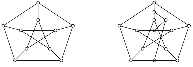
The class of graphs that do not contain a cycle with a unique chord, also known asunichord-free graphs, is studied by Trotignon and Vuˇskovi´c in [119], where they obtain the following structure theorem for this class.

Figure 3: Petersen and Heawood graph

The Petersen and Heawood graphs are the two famous graphs, depicted in Figure 3, that were discovered at the end of the XIXth century in the research on the four color conjecture ([103], [79]), and they also appear as basic classes of

unichord-free graphs. A graph is strongly 2-bipartite if it is 4-hole-free and bipartite with

bipartition (X, Y) where X is the set of all degree 2 vertices of G and Y is the set

of all nodes ofGof degree at least 3. A node cutsetS ={a, b}of a connected graph

Gis aspecial 2-cutset ifaandb are nonadjacent and both of degree at least 3, and

such thatV(G)\Scan be partitioned intoX andY so that: |X| ≥2,|Y| ≥2; there

are no edges betweenX andY; and bothG[X∪S] andG[Y ∪S] contain anab-path.

A 1-join with split (X1, X2, A1,∅,∅, A2,∅,∅) is properif both A1 and A2 are stable

sets of size at least 2.

Theorem 7.3 (Trotignon and Vuˇskovi´c [119]) A connected unichord-free graph either has a 1-cutset, a special 2-cutset, or a proper 1-join, or is one of the following types:

• a clique,

• a strongly 2-bipartite graph, or

• an induced subgraph of the Petersen or the Heawood graph.

We note that the decomposition theorem above in fact implies a complete struc-ture theorem for unichord-free graphs. The decompositions in Theorem 7.3 can be reversed into compositions in such a way that every unichord-free graph can be built starting from basic graphs, that can be explicitly constructed, and gluing them to-gether with prescribed composition operations, and all graphs built this way are unichord-free. This also implies a straightforward decomposition based recognition

algorithm for this class that runs in O(nm) time.

Since unichord-free graphs are diamond-free, any edge of a unichord-free graph is contained in a unique maximal clique. Hence to find a maximum clique it is

enough to look for common neighbors of every edge. This leads to anO(nm) time

algorithm. In [119] anO(n+m) algorithm is given for the maximum clique problem

for unichord-free graphs. It is based on the fact that a connected unichord-free graph that contains a triangle is either a clique or has a 1-cutset. Also in [119] it is shown

how Theorem 7.3 can be used to obtain anO(nm) coloring algorithm for

unichord-free graphs. It turns out that every unichord-unichord-free graph G is either 3-colorable or

has anω(G)-coloring, and in particular χ(G)≤ω(G) + 1. The problem of finding a

maximum stable set of a unichord-free graph is NP-hard (follows from 2-subdivisions [105]).

Another characterization of unichord-free graphs is given by McKee in [97]: unichord-free graphs are precisely the graphs whose all minimal separators are stable

sets (where a separator in a graph G is a set S ⊆V(G) such that G\S has more

connected components thanG).

7.3 Propeller-free graphs

Motivated by trying to understand the structure of wheel-free graphs, whose recognition remains an open problem, Aboulker, Radovanovi´c, Trotignon and Vuˇskovi´c

studied in [3] a subclass of wheel-free graphs known aspropeller-free graphs. A

pro-peller is a a graph that consists of a cycle C and a node x that has at least two

neighbors onC. Let C0 be the class of graphs that have no node that has at least

two neighbors of degree at least 3, C1 the class of graphs that have no propeller as

a subgraph, andC2 the class of propeller-free graphs. ClearlyC0 (C1(C2.

First let us point out that by considering a longest path it is easy to show that

graphs in C2 must always have a node of degree at most 2, and hence they are

3-colorable, see [3]. Observe that since a clique on 4 nodes is a propeller finding the size of a largest clique in a propeller-free graph can easily be done in polynomial time. On the other hand, finding a maximum independent set of a propeller-free graph is NP-hard (follows easily from [105], see also [119]).

The following decomposition theorems are given in [3], and used to obtain an

O(nm) recognition algorithm for class C1, and an O(n2m2) recognition algorithm

for classC2.

A 2-cutset {a, b} of a graph G is an S₂-cutset (resp. K₂-cutset) if ab is not

an edge (resp. is an edge). An S2-cutset is proper if nodes of G\ {a, b} can be

neitherG[X∪ {a, b}] nor G[Y ∪ {a, b}] is a chordless ab-path. AK2-cutset isproper

if G\ {a, b} contains no node adjacent to both a and b. A 3-cutset {u, v, w} of a

graphG is anI-cutset ifG[{u, v, w}] contains exactly one edge.

Theorem 7.4 (Aboulker, Radovanovi´c, Trotignon and Vuˇskovi´c [3]) A con-nected graph inC1 is either inC0 or it has a 1-cutset, a properK2-cutset or a proper S2-cutset.

Theorem 7.5 (Aboulker, Radovanovi´c, Trotignon and Vuˇskovi´c [3]) A graph in C2 is either in C1 or it has an I-cutset.

Furthermore, it is shown in [3] that propeller-free graphs admit an extreme de-composition, which is used to prove that 2-connected propeller-free graphs must always have an edge whose endnodes are of degree 2. This implies that propeller-free graphs can also be edge-colored in polynomial time.

8 (3P C(∆,·),proper wheel)-free

Let (H, x) be a wheel. A sectorof (H, x) is a minimal subpath of H, of length

at least one, whose endnodes are neighbors of x on H. A sector is short if it is

of length one, and long otherwise. (H, x) is a triangle-free wheel if it has no short

sectors. (H, x) is a universal wheel ifx is adjacent to all nodes of H, i.e. it has no

long sectors. (H, x) is a line wheel if it has four sectors, exactly two of which are

short, and the short sectors have no common node. (H, x) is afanned wheelif it has

exactly one long sector. Aproper wheel is a wheel that is not a triangle-free wheel,

a universal wheel, a line wheel, or a fanned wheel with 2 or 3 short sectors. We

now consider three different subclasses of the class of (3P C(∆,·),proper wheel)-free

graphs.

8.1 Cap-free graphs

Acapis a hole together with a node that is adjacent to exactly two adjacent nodes

on the hole. Cap-free graphs were studied in [43], where the focus was on obtaining polynomial time algorithms for recognizing whether a cap-free graph contains an odd (respectively even) hole. Note that the only Truemper configurations that cap-free

graphs can contain are 3P C(·,·)’s and wheels that are either triangle-free, universal

or fanned with exactly two short sectors. The following decomposition theorem is obtained in [43] for this class, generalizing the decomposition theorem for Meyniel graphs obtained by Burlet and Fonlupt in [7].

A graph G contains a 1-amalgam (or amalgam) (X1, X2, K, A1, A2) if V(G) =

X1 ∪X2 ∪K, where X1, X2 and K are disjoin sets, |X1| ≥ 2, |X1| ≥ 2 and the

nodes of K induce a clique inG (possibly K is empty). Furthermore, for i= 1,2,

∅ 6=Ai ⊆Xi; every node of A1 is adjacent to every node of A2, and these are the

only edges between X1 and X2; and every node of K is adjacent to every node of

A1 ∪A2. Amalgams were first introduced in [7], and they generalize 1-joins, as a

1-amalgam with K=∅corresponds to a 1-join.

Abasic cap-free graphGis either a triangulated graph or a biconnected triangle-free graph with at most one additional node, that is adjacent to all other nodes of

Theorem 8.1 (Conforti, Cornu´ejols, Kapoor and Vuˇskovi´c [43]) A cap-free graph is either basic or it has a 1-amalgam.

Cap-free graphs can easily be recognized in polynomial time directly, but in [43] Theorem 8.1 is used to obtain decomposition based recognition algorithms for cap-free even-signable and cap-free odd-signable graphs (even-signable graphs are a generalization of odd-hole-free graphs, and odd-signable graphs are a generalization of even-hole-free graphs; they are formally defined in Section 9).

Since triangle-free graphs are cap-free (basic), it follows that the problems of coloring and finding the size of a largest independent set are both NP-hard for cap-free graphs. On the other hand, it is easy to see how to use Theorem 8.1 to obtain a polynomial time algorithm to solve the maximum weight clique problem for cap-free graphs, see [51].

Theorem 8.1 is a generalization of analogous result obtained by Burlet and

Fonlupt [7] for Meynielgraphs, which are exactly (cap, odd-hole)-free graphs. The

decomposition of Meyniel graphs by 1-amalgams is used in [7] to obtained the first known polynomial time recognition algorithm for this class. Subsequently, Rous-sel and Rusu [113] obtained a faster algorithm for recognizing Meyniel graphs (of

complexityO(m2)), that is not decomposition based.

Hertz [80] gives anO(nm) algorithm for coloring and obtaining a largest clique

of a Meyniel graphs. This algorithm is based on contractions of even pairs. Roussel

and Rusu [114] give anO(n2) algorithm that colors a Meyniel graph without using

even pairs. This algorithm “simulates” even pair contractions and it is based on lexicographic breadth-first search and greedy sequential coloring. In [9] Cameron,

L´evˆeque and Maffray give another O(n2) algorithm for coloring Meyniel graphs,

which takes as input any graph and finds either a clique and a coloring of the same size or a Meyniel obstruction (i.e. an odd cycle of length at least 5 with at most one chord).

Conforti and Gerards [51] show how to obtain a polynomial time algorithm for solving maximum weight independent set problem, on any class of graphs that is decomposable by amalgams into basic graphs for which one can solve the max-imum weight independent set problem in polynomial time. In particular, using Theorem 8.1, they obtain a polynomial time algorithm for solving the maximum weight independent set problem for (cap, odd-hole)-free graphs (i.e. Meyniel graphs) and (cap, even-hole)-free graphs (and more generally, cap-free odd-signable graphs). Whether (cap, even-hole)-free graphs can be colored in polynomial time remains an open problem.

8.2 Claw-free graphs

A claw is a complete bipartite graph K1,3. Observe that claw-free graphs are

3P C(·,·)-free and the only wheels they may contain are line wheels, universal wheels

whose rim is of length 4 or 5, and fanned wheels with 2 or 3 short sectors.