Interferometric measurement of ionization in a grassfire

O R I G I N A L P A P E R

Interferometric measurement of ionization in a grassfire

Kgakgamatso Marvel Mphale•_{M. Heron}•

R. Ketlhwaafetse•_{D. Letsholathebe}•

R. Casey

Received: 26 May 2006 / Accepted: 14 January 2010 / Published online: 3 February 2010 ÓSpringer-Verlag 2010

Abstract Grassfire plumes are weakly ionized gas. The ionization in the fire plume is due to thermal and chemi-ionization of incumbent species, which may include gra-phitic carbon, alkalis and thermally excited radicals, e.g., methyl. The presence of alkalis (e.g., potassium and sodium) in the fires makes thermal ionization a predominant electron producing mechanism in the combustion zone. Alkalis have low dissociation and ionization potentials and therefore require little energy to thermally decompose and give electrons. Assuming a Maxwellian velocity distribution of flame particles and electron-neutral collision frequency much higher than plasma frequency, the propagation of radio waves through a grassfire is predicted to have attenuation and phase shift. Radio wave propagation measurements were performed in a moderate intensity (554 kW m-1) controlled grassfire at 30- and 151-MHz frequencies on a 44 m path using a radio wave interferom-eter. The maximum temperature measured in the controlled burn was 1071 K and the observed fire depth was 0.9 m. The radio wave interferometer measured attenuation coefficients of 0.033 and 0.054 dB m-1for 30- and 151-MHz, respec-tively. At collision frequency of 1.091011s-1, maximum electron density was determined to be 5.06191015m-3. List of symbols

c Speed of light in vacuum (m s-1)

d Propagation path length (m)

Dc Degree of curing (%)

e Electron charge (-1.691019C)

f0 Propagation frequency (s -1

)

Fd Flame depth (m)

me Mass of electron (9.1910-31kg)

Msad Mass of dried sample (kg) N Electron density (m-3)

r Residual fuel load (kg m-3) RoS Rate of spread (m s-1)

Rx Receiver

tr Resident time (s)

Tx Transmitter

Hc Heat of combustion (J/kg)

Ig Fire line intensity (kW m-1)

W Fuel load (kg m-3)

U1.5 Windspeed at 1.5 m above ground (m s-1) U2 Windspeed at 2 m above ground (m s-1) U10 Windspeed at 10 m above ground (m s-1)

Greek symbols

af Flame attenuation coefficient (Np m-1) b0=2pf0/c Phase constant in vacuum (rad m-1) bf Flame phase coefficient (rad m-1) e0 Permittivity in free space (H m-1)

~

ceff Propagation constant

D/ Phase change (rad m-1)

ueff Effective collision (rad s -1

)

x Radial propagation frequency (rad s-1)

xp=(ne2/mee0)1/2 Plasma frequency (rad s-1)

1 Introduction

Wildfire management agencies in Australia are concerned about radio wave communication reliability in extreme fire K. M. Mphale (&)R. KetlhwaafetseD. Letsholathebe

Physics Department, University of Botswana, P/Bag 0022, Gaborone, Botswana

e-mail: Mphalekm@mopipi.ub.bw

M. HeronR. Casey

Marine Geophysical Laboratory, James Cook University, Townsville, QLD 4811, Australia

conditions (Boan2007; Griffiths and Booth2001). Several cases of failure to maintain radio wave communication at high frequency (hf) to very high frequency (vhf) through and in close proximity of wildfires have been reported in Australia, e.g., during the Lara bushfire disaster of 1969 (Williams et al.1970) and Dwellingup bushfire disaster of 1961 (Foster 1976). An explanation of how this could happen is still sought. Williams et al. (1970) and Hata and Shigeyuki (1983), who studied super high frequency (shf) propagation in mass wildfires, attributed radio wave signal loss in wildfires to refraction and ionization in the fires. The researchers acknowledged that very high intensity wildfires could significantly affect radio signal strength due to heat-generated weakly ionized plasma in the plume. The generated plasma may lead to communication malfunction or even blackout (see for example, Hofmann1966).

A chemi-ionization reaction, which involves excited methyl (CH*) radical and oxygen atom (O) is a known source of electrons in unseeded hydrocarbon flames (Butler and Hayhurst1998; Alkamade et al. 1982). The reaction occurs in the flame’s primary combustion zone where temperatures are in excess of 1000°C. However, in flames such as moderate intensity wildfires, the reaction could be hindered by the availability of O atoms as the parent molecule (O2) has high dissociation energy. Other sources

of free electrons in unseeded flames are coagulated forms of carbon; graphite and soot, which are produced in sig-nificant quantities in wildfires (see Preston and Schmidt

2006). The carbon forms produce electrons by thermionic emission as they have low work functions (Sodha et al.

1963). The work function values for graphite and soot have been determined to be 4.35 and 8.5 eV, respectively (Shuler et al. 1954). In hydrocarbon flames seeded with alkali metals, the latter species become dominant electron sources. This is due to the fact that the species have low ionization energies, e.g., potassium has first ionization energy of 4.35 eV (Semenov and Sokolik1970). Wildfires are essentially hydrocarbon flames seeded with alkali-based nutrients (Mphale and Heron2007).

The vegetation contains alkali and alkaline earth metal (AAEM) species as part of inherent inorganic ash. The AAEMs are mainly salts of potassium, calcium and sodium, which exist in different physical forms, with the species of potassium being a larger fraction of the inor-ganic ash. AAEMs can exist; ionically or orinor-ganically attached to oxygen-containing functional groups (i.e.,-O– C-) of the organic structure of plants, as discrete particles in voids of the organic matrix and in solution form such as in xylem vessels. During a wildfire, AAEMs are released from a thermally crumbling plant structure and convec-tively drawn into the combustion zone of the fire. As potassium species form a larger fraction of the omnipresent inorganic particulates in plants, they are also a large

fraction of inorganic emissions during plant matter com-bustion (Knudsen et al. 2004). The wildfire combustion zone is characterized by sufficiently high temperatures to cause thermal dissociation and ionization of alkalis (Vod-acek et al. 2002). From studies of nutrient cycling, up to 28% of inherent potassium in plants is volatilized at a combustion efficiency of 98% (Raison et al. 1985). Vod-acek et al. (2002) also estimate that 10–20% of potassium in vegetation is ionized in wildfires. Alkalis are estimated to produce electron densities in the range 1014to 1017m3 in wildfires (Boan2006; Mphale and Heron2007).

Electromagnetic wave propagation in weakly ionized gas is controlled by the medium’s constitutive parameters, which are a factor of electron density and collision fre-quency (Zivanovic et al. 1964). However, at radio wave frequencies, the interaction of signals with a weakly ion-ized gas is mainly dependent on its electron density (Guo and Wang 2005). The higher the electron density, the higher will be the radio wave signal absorption. The paper reports on line-of-sight (LOS) signal amplitude measure-ments carried out at hf (30 MHz) and vhf (151 MHz) in a moderate intensity grassfire plume. The frequency bands used in the experiment were chosen for their relevance to fire fighting communication systems in rural Australia. In the experiment, signal phase change is also measured to further characterize the effect of fire on radio wave signals. Wildfire ionization was then determined from the measured parameters. Electron density measurements in wildfires are essential for fire–radio wave interaction model validation and numerical propagation prediction studies in similar environments.

2 Ionization in wildfire

There are two mechanisms that are responsible for wildfire plume ionization; these are thermal and chemical ioniza-tion processes (see Latham 1999). In thermal ionization, plume particles are selectively ionized based on both the temperature and ionization potential. Species with low ionization potential in a high temperature environment are easily ionized. Ionization by the processes could be determined using the Saha equation (Haught1962). In the combustion zone, the AAEMs are dissociated into atoms. The hot environment excites the atoms, which lose their outer shell electrons according to the following equation (Nesterko and Taran1971):

AM$AMþþe ð1Þ

where AM*, AM? and e- are excited alkali metal, the metal ion and electron, respectively.

ionization reactions. It is known that excited methyl (CH*) radicals, chlorine ions (Cl-), hydrogen atoms (H) and acetylene (C2H2) molecules react with each other to give

electrons in flames (Semenov and Sokolik 1970). The methyl radical reacts with acetylene to give electrons, according to the following equation (Alkamade et al.

1982):

CHþC2H2$C3Hþ3 þe

_{: ð2Þ}

Chlorine ions, which exist in substantial amounts in vegetation fires (Mphale 2008), react with hydrogen radical to produce hydrogen chloride gas and electrons according to the equation:

HþCl$HClþe: ð3Þ

However, the production of electrons by Eq. (3) could be hampered by the presence of alkalis, which compete for Cl- with the H radical. Alkalis react with chlorine to produce metal chlorides.

3 Radio wave interferometry

3.1 Theory

An interferometer can be arranged to measure both signal attenuation and phase shift at a suitable frequency deter-mined by collision frequency and electron density of a medium under diagnosis (Caron et al. 1968; Howlader et al. 2005). It has advantages over other conventional methods, e.g., use of Langmuir probes, of being non-intrusive and provides a direct measurement of attenuation. The use of Langmuir probes is limited to measuring local electron density and carries with it some inherent problems such as probe heating and local plasma perturbation. At microwave frequencies, an interferometer has been used to measure line-integrated plasma electron density and colli-sion frequency of laboratory-scale weakly ionized plasma (Zivanovic et al.1964; Gilchrist et al. 1997). Apart from being expensive, microwave interferometers are fragile equipment and may not be suitable for outdoor deploy-ment. Diagnosis of large unbound tenuous atmospheric pressure ionized plumes, such as wildfires, may require outdoor deployment of an interferometer. A robust and relatively cheap radio wave interferometer could be appropriate for the task.

At atmospheric pressure, weakly ionized gases, such as flames, are highly collisional with frequencies of about a tenth of a terahertz (1011Hz) (e.g., in Jamison et al.2003). When the probe signal of an interferometer is HF or VHF, radio waves (ueff/x)[1 and (xp/x)[1. In this case,

propagation theory, e.g., in Hofmann 1966, predicts transmission through a wildfire with significant attenuation.

Consider a plane polarized radio wave to traverse a weakly ionized flame medium of average propagation path length din the positivex-direction, then its amplitude (Ef) is given by the relation (Santoru and Gregorie1993):

EfðxÞ ¼E0exp Zd

0

~ ceffðxÞdx 8

< :

9 =

; ð4Þ

where E0 is free space electric field strength of the

electromagnetic signal. The effective propagation constant ~ceff

ð Þis complex and is related to attenuation (af) and shift

(bf) coefficients in the flame medium by the expression

(Laroussi and Roth 1993): ~

ceff¼afþibf: ð5Þ

Based on high collisionality and weak ionization in fire medium, Mphale and Heron (2007) approximated radio wave propagation coefficientsafandbfin (5) as:

af ffi x

c

x2 p

2xueff

" #

ð6Þ

and

bf ffi x

c 1þ

x4 p

8u2 eff

1

x2

" #

ð7Þ

The attenuation and phase coefficients in (6) and (7) provide useful information about the electromagnetic properties (electron density and collision frequency) of the medium, e.g., in Akhtar et al.2003and Koretzsky and Kuo (1998).

Considering the real part of Eq. (4), radio wave signal attenuation is determined from signal intensity in free space relative to that in fire medium and is given by the following expression (Schneider and Hofmann1959):

Attn dBð Þ ¼10 log₁₀ E0

Ef

2

( )

Attn dBð Þ ¼20 log₁₀eafd

ð8Þ

Induced phase change is related to phase coefficient in free space and that in fire medium and is given by the expression (Howlader et al.2005):

D/¼ Zd

0

bf b0

ð Þdx

D/¼x

c Zd

0

1þ x 4

p 8u2 eff

1

x2

" #

1

( )

dx

ð9Þ

D/¼fbfb0gd¼ e2

16cpm2 ee20

n2_d f0u2eff

D/¼0:00067 n

2_d

f0u2_eff

ð10Þ

and attenuation=afd; therefore afd¼

e2

2cmee0 nd ueff

¼5:292106nd

ueff

ð11Þ

Dividing Eq. (10) by (11) gives electron density as:

n¼0:0079f0ueff

D/

Attn ð12Þ

Uhm (1999) relates flame gas collision frequency to its temperature by the relation

ueff ¼1:3610 12Tr

Tg

Te

ð Þ1=2 ð13Þ

whereTr,TgandTeare ambient, flame and electron tem-peratures, respectively. Sicha (1979) observed that electron temperature in flame at about 1000 K is 0.1 eV.

3.2 Radio wave interferometer

Radio wave interferometer is an instrument designed to use the same principles as the microwave interferometer except that it works at a much lower frequency and is suitable for measuring ionization of large unbounded volumes of

slightly ionized gases at atmospheric pressure such as wildfires.

The interferometer has six units whose primary func-tions are to synthesize, transmit, receive and process phase coherent radio signals. The units perform the above func-tions on 6-, 30- and 150-MHz signals. The block diagram in Fig.1 shows all the units making up the radio wave interferometer. The specific functions of the units are dis-cussed in Sect.4.4.

4 Experimental methods

4.1 Prescribed grassfire

4.1.1 Study site and vegetation structure

The study site was located at 147°580₅₆00_{E and 19°25}0₄₆00_S

on the western side of James Cook University’s main campus in Townsville, Queensland. The climate in the Townsville region is warm and humid (Lokkers 2000). Summers are hot with an average maximum temperature of 30.7°C in January. An average minimum temperature of 15.4°C occurs in winter (July). The region receives an average annual rainfall of 1143 mm (Williams et al.2003). Most of it falls during summer; a season that extends from December to March. The rainfall in this season is generally associated with the northeasterly trade winds, cyclones and

30MHz 75MHz

Oscillator

6MHz X2

1/5 A

A 1/5

X 2

Lo Frequency Generator

6MHz X 4 X 6 6MHz RF Amp

30 MHz Reciever

150MHz Φ Φ Comp

150MHz Amplitude

150MHz Φ Comp. 30MHz Φ Φ Comp

30MHz Amplitude

30MHz Φ Comp.

6MHz RF Amp

150 MHz Reciever Oscilloscope

Master Oscillator Transmitter Unit

30MHz

30MHz

150MHz 150MHz

24MHz

144MHz

depressions (Lokkers2000). Long dry periods during the winter and variable annual rainfall have resulted in the region being fire-prone, and frequent fires have created mosaics of open forest, woodlands and grasslands in the region.

The vegetation structure in the study site consists of open woodlands of eucalyptus and grassy understorey. The understorey is mainly black spear grass and there are occasional 1.5–3 m high chinee-apple shrubs. The average spear grass density and height were 150 plants/m2 and 1.0 m, respectively. The dominant overstorey tree species were poplar gums eucalyptus (see Fig.2).

The site was irregular in shape (see Fig.9) with a perimeter of 393 m. A propagation path of about 44 m long was chosen at the site in an area where there was minimum obstruction from trees and shrubs. The site was chosen along with others by the Physical Planning Division of the University for Controlled burning in 2004, a preemptive exercise necessary for the control of high intensity wild-fires occurrence on the campus. The amount of fuel accu-mulated and the proximity to building structures were the main reasons for the selection of these plots.

4.1.2 Fuel characteristics

Vegetation was sampled by means of 1 m2quadrants. Four 1 m2quadrants were randomly set up 1 h before ignition in the prescribed burn area. Twenty (20) spear grass plants were randomly sampled in each quadrant. The height of each plant was measured by a 5-m measuring tape and then averaged to give the average fuel height (Ha). Surface litter and vegetation (clipped from just above the ground sur-face) were collected from the quadrants into separate bags (a bag for each quadrant) and then sealed for analysis. The mass of plant material from each quadrant was determined and the masses were then averaged to give W. Weighed

samples of plant material from each bag were then dried in an oven set at 60°C for 72 h. The oven-dried plant mate-rials were thereafter re-weighed to give dry mass, which averaged to give Msad. The degree of curing (Dc) for the fuel was determined from the relation:

Dc¼ 1

WMsad W

100% ð14Þ

Fuel load (FL) for the study area was calculated from the averaged biomass per unit area; thus

FLðkg/m2Þ ¼W: ð15Þ

4.2 Measurement of grassfire behavior

The magnitude of radio wave signal attenuation is depen-dent on fire behavior (i.e., intensity and fire depth), e.g., in Boan (2007). Therefore, it is important that the grassfire behavior is fully characterized in the experiment for the attributes to be related to the measured attenuations. In the controlled burn, fire was ignited such that its front was in the direction of the prevailing wind. During the experi-ment, wind blew from the northeast direction (60°E) (see Fig.3). The propagation equipment was set such that radio waves propagate approximately in the west to east direc-tion. The rate of spread (RoS) for the grassfire was deter-mined from running the CSIRO Fire Spread Calculator v.1 (CSIRO 1998). Fire Spread Calculator is a WindowsÒ based program that calculates RoS for different vegetation scenarios in Australia including northern Australia’s open woodland vegetation. The inputs to this model are ambient temperature, relative humidity, curing percentage and wind speed (km/h) at 10 m. From the RoS determined from the Fire Spread Calculator, the flame depth of the grassfire was

Fig. 2 Vegetation structure at the study area

N

Wind (60°E)

Tt

30°

Fd A

B

D C

G E

Direction of grassfire

calculated by considering that the flame front intercepted the transmission path at an angle of 30°(Fig.3).

Noting that the grassfire was frontal or line fire, its flame depth (Fd) was proportional to flame residence time (tr) or the time the flame took to cross the propagation path. The constant of proportionality is the RoS; thus

Fd¼RoStr ð16Þ

Residence time (tr) for the flame is to be determined from radio wave propagation measurements. By inspection angle DAB in Fig.3 is 30°. Also from the figure, Fd can be calculated as follows:

Fd ¼ABsin 30ð Þ

Fd ¼ð1=2Þ AB

ð17Þ

From Eqs. (16) and (17), the rate of spread (RoS) is given by

RoS¼AB

2tr

ð18Þ

The intensity of the grassfire is calculated from Byram’s fire line intensity relation given by Sullivan (1997) as:

Igf¼HðWrÞ RoS ð19Þ

where r is residual weight. It was observed that during the controlled burn, all of the surface fuel burnt; thus,

r&0 in (19).

4.3 Temperature measurements

Grassfire caused signal attenuation occurs when the fire crosses the propagation path. The interception can be detected by putting thermal sensors (thermocouples) in the propagation path ahead of the fire front. A signal attenua-tion, which occurs at the same time with the measured temperature maxima, could then be assumed to be caused by fire and hence the need for temperature measurements in the experiment.

A thermocouple tree of about 1.25-m high was con-structed from a steel pipe of diameter 0.025 m (see Fig.4). Steel rods (arms) of length 0.4 m were attached at every 0.25 m of the tree’s height to hold up to five thermocou-ples. Thermocouples were cut from a 100-m double braided fiberglass-insulated chromel–alumel (24-G/G) thermocouple wire, 50lm in diameter. The thermocouple wire has a fiberglass shield, which can withstand temper-atures up to 450°C. At tempertemper-atures greater than 450°C, the fiberglass shield fuses. Our tests showed that the insulation properties hold for higher temperatures, but the material then becomes brittle on cooling, and therefore can be used only once.

The type K thermocouple wires were electro-fused at one end to make perfect junctions and tested with a hot

air gun and a multimeter. The thermocouples were then fixed to tree arms by means of muffler tape, and the electro-fused junctions were left protruding 0.01 m beyond the arm length into the flame. The thermocouple wires were buried in a shallow trench (0.1 m deep) and connected to the thermocouple logger 3 m away from the thermocouple tree at a spot that allowed access without trampling the fuel in the immediate vicinity of the thermocouples.

The thermocouples were wired to a SPECTRUMÒ SP 1700-51W thermocouple data logger to read in tempera-tures into the data logger’s internal memory throughout the experiment. Operational cold junction temperature of the data logger ranges from -45 to 85°C; therefore, it was necessary to protect the logger from heating beyond 85°C, as this may invalidate the data. The data logger was dug 0.75 m into the ground and wrapped around with an insulating material (FiberflexÒ) to protect it from heat that may the produced in the grassfire. SP 1700-51W log-ger has the capability to read temperatures up to 1370°C and is therefore ideal for measuring bushfire flame temperatures.

4.4 Interferometer units

4.4.1 Master oscillator and transmitter unit

The unit is responsible for generating phase coherent 6-, 30- and 150-MHz radio wave signals from a 75-MHz master oscillator. A 75-MHz square wave signal is fre-quency divided by 5 using logic circuits; it is then doubled (92) to produce a 30-MHz sinusoidal signal. The 30-MHz signal is then amplified to a power rating of 250 mW and fed to a 30-MHz antenna. A part of the 30-MHz signal is

Spectrum 1700 logger Thermocouple

Tree

Cable

Cable for Phase Measurement

Direction of Fire Front

0.75m 0.20m

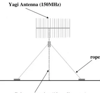
tapped, buffered and then divided by 5 to produce a 6-MHz reference signal. This reference signal is fed at low impedance to a 75-m long coaxial cable and connected to the receiver unit (Rx). The 75 MHz was doubled to produce a 150-MHz sinusoidal signal. It was then amplified and fed to a 150-MHz Yagi antenna. The unit produced phase-coherent signals, since they were produced from one oscillator: the 75-MHz master oscillator.

4.4.2 Local oscillator generator (LOG) and receiver (Rx) units

The main function of these units is to receive the trans-mitted signals from the master oscillator–transmitter unit and synthesize a 6-MHz signal for phase comparison. Generally, LOG generates signals for mixing in the Rx units. The LOG unit is fed with the 6-MHz reference signal from the master oscillator and transmitter unit. The refer-ence signal is frequency-multiplied by 4 and 6, respec-tively, to produce 24- and 144-MHz signals (Fig.4). In the 30-MHz Rx unit, a received signal from the 30-MHz antenna is mixed with a 24-MHz signal from the local oscillator frequency generator to produce 6 MHz. The 150-MHz signal received from a Yagi antenna is mixed with a 144-MHz signal from the LOG to produce 6 MHz. The 6-MHz signals and the reference 6 6-MHz are fed in respective phase comparators.

4.4.3 Comparators

These are 180°phase comparison circuits. The phase of 6-MHz signals fromRxunits is compared with the phase of the 6-MHz reference. A DC voltage representative of this phase difference is registered in a HOBOÒ data logger. Initially, a voltage of 2.5 V was set for the 180° phase difference.

4.4.4 Antennae

Two types of antennae were used in the interferometer; a horizontal Yagi (Fig.5) and vertical quarter-wavelength whip (Fig.6). The Yagi antenna was designed to work at a frequency range of 149–151 MHz, and the vertical quarter-wavelength whip at 30 MHz.

The Yagi antenna had a highly directional type of radiation pattern. At near field, a nominal gain of the antenna was 11.4 dBd. From its radiation pattern in the E-plane, 3 dB was at 34°, while the pattern in the H-E-plane, 3 dB was at 43°. Radiation pattern for the 30-MHz quarter wavelength whip antenna was omnidirectional.

4.4.5 Phase change tests and calibration of comparator unit

The interferometer was tested for sensitivity to phase changes using antenna position shifts. In the tests, an oscilloscope was used to monitor the output from the 30-MHz phase comparator unit. The quarter wave dipole was initially set at position A (PsA) so that the amplitude signal and the reference signal (shown as a square wave in Fig.7a) were in phase. The antenna was moved a fraction of the wavelength away from PsA. When the antenna was moved 2.9 m (0.29k) away from PsA, a phase shift of 55° was induced (calculated from Fig.7b). Theoretically, a phase shift of 54° should be imposed on the radio wave; therefore, the comparator circuit responded very well to the change in the antenna position.

When the antenna was moved 5.0 m (0.5k) away from PsA, a phase shift of 90° was induced on the amplitude signal (as calculated from Fig.8b).

Fig. 5 A 150-MHz Yagi antenna

4.5 Radio wave propagation measurements

4.5.1 Propagation and phase measurement path

The transmitters and receivers were set up on opposite sides of the plot, separated by a direct distance CA–CD (Figs.9,

10) of 44 m. A 75-m long 75Xcoaxial cable used for phase change measurement was dug 0.20 m in the ground. The purpose of the trench was to protect the cable from the heat that may diffuse into the ground. At this depth, the heat from the grassfire is negligibly small that it cannot influence the phase measurements. During the propagation measure-ment, the cable ran far from where the head fire intercepted the transmission path. The cable was set such that CD–CC was 10.3 m, CC–CB was 25.5 m and CB–CA was 9.5 m to connect to both 30-MHz receiver and transmitter units.

The transmitter, receiver and the rest of the units were enclosed in polysterene boxes to prevent heat from the fire affecting the circuitry. A polystyrene board was placed over the boxes to act as shade for both the boxes and the cables that connect to the antennas. The boards were placed over the boxes in such a way that it allowed circulation around the enclosures. A thermocouple was connected to a HOBOÒdata logger and placed inside the boxes to monitor the temperature inside the boxes.

4.5.2 Signal amplitude measurement

The 150- and 30-MHz modules were tested for stability days before the controlled burn. It was noted that the 150-MHz module was not stable; only the 30-150-MHz module passed the test. The 150-MHz module was replaced by a

Fig. 7 Phase change due to moving the antenna:aphase at the starting position (PsA) and

bantenna moved 2.9 m away from the starting position

Fig. 8 Phase change due to moving the antenna:aphase at the starting position (PsA) and

bantenna moved 5.0 m away from the starting position

189m

100m 92m

N

12m

CB

CA

CC CD

Tx

Rx

Wind

Tt

commercial 151-MHz module and we had to cancel the phase measurements at this frequency.

The 30- and 151-MHz modules were set (on different days) and left to run for a period of 2572 and 1209 min, respectively. It was observed that the 30-MHz signal fluc-tuated around an average amplitude of 2011.06 mV with the maximum and minimum amplitudes of 2011.32 and 2010.80 mV, respectively. Standard deviation from the mean amplitude was calculated to 0.10 mV(±0.001 dB). The 151 MHz fluctuated from average amplitude of 899.17 mV with maximum and minimum amplitudes of 899.44 and 898.90 mV, respectively. The standard devia-tion of the signal from its mean amplitude was 0.13 mV(±0.003 dB). It is interesting to note that the signal fluctuations were random and occurred both during the night and day and therefore cannot be alluded to variations in humidity and temperature during the cycle. Besides, the propagation distance (41 m) was too short to consider sig-nificant refractive effects on the signals.

5 Experimental results and discussions

5.1 Grassfire temperature

There is a discrepancy between the actual combustion gas temperature and that measured by a bare bead ther-mocouple (Dupuy et al.2003; Brohez et al. 2004). The error is mainly due to the convection and radiation heat transfer to and from thermocouple bead. The error, which could be up to 200 K, is also attributable to bead phys-ical characteristics such as emissivity and size (Shannon and Butler 2003). However, the actual flame gas tem-peratures could be reconstructed from thermocouple readings using heat balance equation. The discrepancy between the actual combustion gas and thermocouple measured temperature is given by Silvani and Morandini

2009 as

TcgTtc¼

retc 1ecg

T_cg4

htcþ4retcTcg3

ð20Þ

where hc=kNu/dtbis the heat transfer coefficient. Nu, k

anddtbare Nusselt number, diffusivity and bead diameter,

respectively. Diffusivity is related to the specific heat capacity (Cp) and Prandtl number (Pr) by the relation,

k=lCp/Pr. For combustion gases,Pr is 0.71. Following Dupuy et al., Eq. (20) is solved for Tcg, which is actual

flame gas temperature, and this correction was applied on the thermocouple measured temperature. With this cor-rection, it was observed that the discrepancy is more than 40 K for temperatures above 500 K.

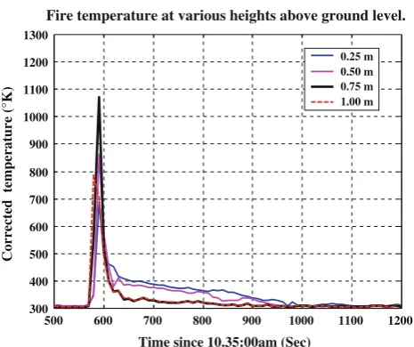
The maximum corrected thermocouple temperature measured in the grassfire was 1071 K. This occurred at 0.75 m above the ground surface at 10.44:50 a.m. It coincided with maximum temperatures at heights 0.25 and 0.50 m above the ground, which were 689 and 862 K, respectively. At 1.00 m, the maximum temperature occurred between 10.44:40 and 10.44:50 a.m. and was 786 K. This was because the flame was wind-blown toward the thermocouple tree, therefore reaching the thermocouple at 1 m earlier than others at lower heights. Considering that flaming combustion occurs at temperatures above 500 K, e.g., in Cruz (2008), therefore from Fig.11and data from the SPECTRUMÒlogger, it can be deduced that the flame residence (tr) time was on average 32 s. This could also be observed from attenuation measurements.

5.2 Attenuation of 151-MHz signal

From the amplitude signal graph (Fig. 12), there was a lot of commotion up to 2 min before the grassfire crossed the propagation path. The signal fluctuations betweenAandB were identified as those due to the university fire sup-pression crew moving up and down a fire break next to receiver units. Fluctuations betweenBandCwere identi-fied as due to a crew member intercepting the propagation

0 500 1000 1500 2000 2500

0.895 0.900 0.905

150 MHz Signal Amplitude (V)

Time since 7:20 am (mins)

signal amplitude

(a)

0 200 400 600 800 1000 1200 2.008

2.010 2.012 2.014 2.016

30 MHz Signal Amplitude (V)

Time since 9:23 am (mins)

signal amplitude

(b)

path at 10.42 a.m. A prominent drop in the signal ampli-tudeD–Ewas observed when the grassfire flame crossed the propagation path. A minute or two after the fire crossed the propagation path, the fire crew moved into extinguish it before it got out of control. This was observed in the drops that occurred in the region E to G of the signal amplitude graph.

The time between 10.42:30 and 10.46:30 a.m. was considered for attenuation calculation as it coincided with temperature maxima measured form the thermocouple tree (Fig.12). Based on the amplitudes between points D and E, attenuation (dB) was calculated using Eq. (8) as signal intensity is directly proportional to voltage.

From Eq. (8), attenuation of the 151-MHz signal due to the flame is:

Attenuation due to the flameðdBÞ ¼20 log₁₀ 0:899 0:894

¼0:048 dB:

Observations reveal that soon after the flame had passed, signal amplitude remained lower than at D. The attenuation could be due to changes in the ground conductivity and scattering, which could have resulted from the removal of ground fuel. Attenuation-due changes in the vegetation cover and conductivity can be estimated to be:

Attenuation due hot flameðdBÞ ¼20 log₁₀ 0:899 0:897

¼0:019 dB:

5.3 Attenuation of 30-MHz signal

The 30-MHz signal responded to path interception in the same way as the 151-MHz signal. Unlike the Yagi antenna used in the 151-MHz transmission, the quarter-wavelength whip used for 30-MHz signals spread energy in all directions. Consequently, reflections from fire crew and their equipment during A–C affected the signal strength more significantly than at 151 MHz (see Fig.13). A prominent drop in the signal amplitude due to the fire was also observed betweenDandE. It occurred at the same time as that of the 151-MHz signal. The vari-ation of the signal amplitude with time graphs is shown in Fig.13.

On comparison of the responses of the 30 and 151-MHz to grassfire interception, it was observed that the 151-MHz signal remained below its average level before the fire, while the 30-MHz signal quickly regained its strength 3 min after the fire.

Attenuation of a 30-MHz signal due to the flame as calculated from Eq. (8) is:

Attenuation due to the flameðdBÞ ¼20 log₁₀ 2:0111 2:0050

¼0:029 dB:

Similarly, that due to the scattering is 0.0022 dB.

500 600 700 800 900 1000 1100 1200

300 400 500 600 700 800 900 1000 1100 1200 1300

Fire temperature at various heights above ground level.

Time since 10.35:00am (Sec)

Corrected temperature (°K)

0.25 m 0.50 m 0.75 m 1.00 m

Fig. 11 Grassfire flame temperatures as they intercepted the propa-gation path

0 200 400 600 800 1000 1200

0.880 0.885 0.890 0.895 0.900 0.905 0.910 0.915 0.920

A

Signal Amplitude Fire Temperature

Time Since 10:35am (sec)

Signal Amplitude (V)

200 300 400 500 600 700 800 900 1000 1100

Fire temperature (K)

Fig. 12 151-MHz Signal amplitude versus time

0 200 400 600 800 1000 1200

2.000 2.004 2.008 2.012 2.016 2.020

signal amplitude fire temperature

Time since 10:35am (sec)

Signal Amplitude (V)

200 300 400 500 600 700 800 900 1000 1100

G

F E D C

B

Fire temperature (K)

A

5.4 30-MHz Signal phase change

The phase on the 30-MHz signal responded in much the same way to path interception by the grassfire front as the amplitude of both the 30- and 151-MHz signals. A prom-inent drop in the signal phase due to the grassfire was observed to be at about 10.44:34 a.m. (Fig.14). It occurred at nearly the same time as the drop betweenDandEfor amplitude attenuation measurement at the two frequencies. The maximum drop for the 30-MHz amplitude occurred at 10.44:45 a.m., while that of 151.3 MHz occurred at 10.44:43 a.m.

The calculated phase shift induced on the 30-MHz sig-nal as worked out from Fig.14 is 32.0 mV. From cali-bration measurement, it was observed that 10.4 mV represents 1°of phase change; therefore, 32 mV is 3.08°. 5.5 Other possible sources of attenuation

and phase changes

Signal attenuation could also be caused by depolarization of radio waves. The depolarization results from scattering of radio waves from vegetation. It increases with frequency for horizontally polarized signal and the reverse is true for vertically polarized waves. It ranges from 0.01 to 0.04 dB/m in moist deciduous and wet evergreen dense tropical forests, respectively (Swarup and Tewari 1979). The experiment was performed in a sparsely vegetated savanna where depolarization is negligible. The influence of carbon soot in the combustion area is insignificant at radio wave

frequencies, but at centimeter wavelengths (Kulemin and Razskazovsky1997).

5.6 Fuel characteristics and grassfire behavior

The fuel characteristics have been calculated from Eqs. (16)–(19), while CSIRO Fire Spread Calculator was used to predict grassfire spread. The inputs to the calculator are: relative humidity; degree of curing; wind speed at 10 m and ambient temperature. Equations (16)–(19) were used to estimate the grassfire front depth. The intensity of the grassfire was calculated using the Byram’s fire-line intensity equation (19).

From the ground data collected at the time of the experiment, it was noted that relative humidity was 37.8%, wind at 1.5 m was 1.0 m/s and ambient temperature was noted to be 28.9°C. Since the fire spread calculator requires wind speeds measurements at 10 m, the wind speed at 2 m can be used to estimate that at 10 m by the use of the relation (CSIRO Fire Spread Calculator 1998):

U101:25U2 ð21Þ

From the wind speed at 1.5 m, a correction for wind speed at 2 m can be done according to the relation given by Cheney et al.(1995) as:

U2¼0:017þ1:056U1:5 ð22Þ

Table1 is a compilation of fuel characteristics and fire behavior as worked from the equations stated.

5.7 Electron density calculation

Propagation measurements show that the 151-MHz signal is the most affected by scattering and changes in the ground conductivity than the 30-MHz one. Attenuation of the 151-MHz signal after the grassfire was nine (9) greater than imposed on the 30-MHz one. Theoretically, attenuation due to the plasma effect imposed on the two frequencies should be of the same magnitude. When compared, the attenuation measurements may imply that a significant portion of 151-MHz signal attenuation may be due to scattering. On the basis of this argument, 30-MHz signal attenuation and phase change measurements are used to determine electron density in the grassfire plume. Applying Eqs. (12) and (13), the calculated electron density was 5.06191015 m-3.

400 600 800 1000 1200

1.320 1.325 1.330 1.335 1.340 1.345 1.350 1.355 1.360 1.365 1.370 1.375 1.380

Phase change Signal Amplitude

Time since 10:35am (sec)

30 MHz Signal Phase Change (V)

2.005 2.006 2.007 2.008 2.009 2.010 2.011 2.012 2.013 2.014 2.015 2.016 2.017 2.018

30 MHz Signal Amplitude (V)

Phase change

Fig. 14 Smoothed signal phase versus time graph

Table 1 Fuel characteristic and fire behavior at plot B

Fuel load (tha-1_{) Curing degree (%) RoS (m/s) Flame depth (m) Est’d. flame height (m) Intensity (kg/m}2_{) (kW/m)}

6 Conclusions

The prescribed grassfire in the experiment was of moderate intensity; thus, Byram’s grassfire intensity was observed to be 554 kW m-1. Maximum temperature measured was 1071 K at 0.75 m above the ground inside the grass fuel stratum. The rate of spread for this fire was approximately 0.06 m s-1. The flame was slightly tilted in the direction of the wind. The grass was 90.1% dry. The depth of the flame was around 0.89 m.

At 151 MHz, maximum attenuation coefficient of the signal intensity due to the grassfire flame was observed to be 0.054 dB m-1. Scattering from hot ground surface after the fire induced a 0.021 dB m-1signal loss. The loss was slightly lower for a 30-MHz signal with a maximum attenuation of 0.033 dB m-1 when it was intercepted by the flame. The hot ground surface also slightly affected the 30-MHz signal as it attenuated the signal by 0.003 dB m-1.

The phase shift induced on the 30-MHz signal was significant. A maximum phase shift of 3.08°was observed as the signal path was intercepted by the grassfire. With this amount of phase shift and the geometry of the exper-iment, it was estimated from Eq. (12) that the maximum electron density in the grassfire was 5.06191015 m-3 when effective collision frequency of 1.291011s-1was used.

Acknowledgments We would like to gratefully acknowledge the Staff Development Office of the University of Botswana for the financial support for this work. The work was partly supported by Emergency Management Australia under project no. 60/2001.

References

Akhtar K, Scharer EJ, Tysk SM, Kho E (2003) Plasma interferometry at high pressures. Rev Sci Instrum 74(2):996–1001

Alkamade CTh, Hollander TJ, Snelleman W, Zeegers PJTh (1982) Metal vapours in flames. Pergamon Press, New York, 460 pp Boan J (2006) Radio communication in fire environments. In:

Proceedings of the Wars 2006 Conference, Leura, NSW, Australia

Boan J (2007) Radio Experiments with fire. IEEE Antennas Wireless Propag Lett 6:411–414

Brohez S, Delvosalle C, Marlair G (2004) A two thermocouples probe for radiation correction of measured temperatures in compart-ment fires. Fire Safety J 39(5):399–411

Butler CJ, Hayhurst AN (1998) Kinetics of gas-phase ionization of an alkali metal, A, by the electron and proton transfer reactions: A?H3O? ? A?.H2O?H; AOH?AOH2??H2O in fuel-rich flames at 1800–2250 K. J Chem Soc Faraday Trans 98:2729–2734

Caron PR (1968) Techniques of measuring the electron density of dense, thick, steady state plasmas. IEEE Antenna Propag Mag 1:611–612

Cheney NP, Gould JS (1995) Fire growth to quasi-steady state rate for forward spread. Int J Wildl Fire 5(4):237–247

Cruz MG, Fernandes PM (2008) Development of fuel models for fire behavior prediction in maritime pine (Pinus pinisterAit) stands. Int J Wildland Fire 17(2):194–204

Dupuy JL, Marechal J, Morvan D (2003) Fires from a cylindrical forest fuel burner: combustion dynamics and flame properties. Combust Flame 135:65–76

Foster T (1976) Bushfire: history, prevention and control. A. H. and A.W. Reed Pty Ltd, Sydney, 26 pp

Gilchrist BE, Ohler SG, Gallimore AD (1997) Flexible microwave system to measure the electron number density and quantify the communications impact of electric thruster plasma plumes. Rev Sci Instrum 68(2):1189–1194

Griffiths B, Booth D (2001) The effects of fire and smoke on vhf radio communications. Country Fire Association, Investigative Report COMM-REP-038-1

Guo B, Wang X (2005) Power absorption of high frequency electromagnetic waves in a partially ionized plasma layer in atmospheric conditions. Plasma Sci Technol 7:2645–2648 Hata M, Shigeyuki D (1983) Propagation tests for 23 GHz and

40 GHz. IEEE J Selected Areas Commun 1(4):658–673 Haught AF (1962) Shock tube investigation of caesium vapour. Phys

Fluids 5(11):1337–1346

Hofmann FW (1966) Control of plasma collision frequency for alleviation of signal degradation. IEEE Trans Commun Technol 3:318–323

Howlader MK, Yang Y, Roth RJ (2005) Time-resolved measurements of electron number density and collision frequencies for fluorescent lamp plasma using microwave diagnostics. IEEE Trans Plasma Sci 33:1093–1099

Jamison SP, Shen J, Jones DR, Isaac RC, Ersfeld B, Clark D, Jaroszynski DA (2003) Plasma characterization with Terahertz time-domain measurements. J Appl Phys 93:4334–4336 Knudsen JN, Jensen PA, Dam-Johansen K (2004) Transformation and

release to the gas phase of Cl, K, and S during combustion of annual biomass. Energy Fuels 18:1385–1399

Koretzsky E, Kuo SP (1998) Characterization of atmospheric pressure plasma generated by a plasma torch array. Phys Plasmas 5:3774– 3780

Kulemin GP, Razskazovsky VB (1997) Radar reflection from explosion and gas wake of operating engines. IEEE Trans Antenna Propag 45:731–739

Laroussi M, Roth JR (1993) Numerical calculation of the reflection, absorption and transmission of microwaves by a non-uniform plasma slab. IEEE Trans Plasma Sci 21:366–372

Latham D (1999) Space charge generated by wind tunnel fires. Atmospheric Res 51:267–278

Lokker C (2000) Draft revegetation strategy for the Townsville City Council. Townsville City Council, Townsville

Mphale KM (2008) Radio wave propagation and prediction in wildfires. PhD thesis, James Cook University, Townsville, QLD Mphale K, Heron ML (2007) Plant alkali content and radio wave communication efficiency in high intensity savanna wildfires. J Atmospheric Solar-Terrestrial Phys 69:471–484

Nesterko NA, Taran EN (1971) Ionization and radiation of alkali metals in acetylene–air flame plasma, with halogen additions. J Appl Spectrosc 14(2):242–244

Preston CM, Schmidt MWI (2006) Black (Pyrogenic) carbon in boreal forests: a synthesis of current knowledge and uncertain-ties. Biogeosci Discuss 3:211–271

Raison RJ, Khaina PK, Woods P (1985) Mechanisms of element transfer to the atmosphere during vegetation burning. Can J For Res 15:132–140

Santoru J, Gregorie DJ (1993) Electromagnetic wave absorption in highly collisional plasma. J Appl Phys 74(6):3736–3743 Schneider J, Hofmann FW (1959) Absorption and dispersion of

Semenov ES, Sokolik AS (1970) Thermal and chemical ionization in flames combustion. Explosion Shock Waves 6(1):33–43 Shannon KS, Butler BW (2003) A review of error associated with

thermocouple temperature measurement in fire environments. Second international wildland fire ecology an fire management congress and fifth symposium on fire and forest meteorology. American Meteorological Society, Orlando, FL, 16–20 Novem-ber 2003, 7B.4, p 3

Shuler KE, Weber J (1954) A microwave investigation of the ionization of hydrogen–oxygen and acetylene–oxygen flames. J Chem Phys 22:491–502

Sicha M (1979) Measurement of the electron energy distribution function in a flame plasma at atmospheric pressure. Czechoslo-vak J Phys 29:640–645

Silvani X, Morandini F (2009) Fire spread experiments in the field: temperature and heat fluxes measurements. Fire Safety J 44:279– 285

Sodha MS, Palumbo CJ, Daley JT (1963) Effect of solid particle on electromagnetic properties of rocket exhaust. Br J Appl Phys 14:916–919

Sullivan AL (1997) Convective Froude and Byram’s energy criterion for Australian experimental grassland fires. Proc Comb Inst 31:2557–2564

Swarup S, Tewari RK (1979) Depolarization of radio waves in jungle environment. IEEE Trans Antennas Prop 27(1):113–116 Uhm HS (1999) Properties of plasmas generated by electrical

breakdown in flames. Phys Plasmas 6(11):4366–4374

Vodacek A, Kremens RL, Fordham SC, VanGorden SC, Luisi D, Schott JR, Latham DJ (2002) Remote optical detection of biomass burning using potassium emission signature. Int J Remote Sens 23(13):2721–2726

Williams DW, Adams JS, Batten JJ, Whitty GF, Richardson GT (1970) Operation Euroka: An Australian Mass Fire Experiment. Report 386, Maribyrnor, Victoria, Australia, Defense Standards Laboratory Williams RP, Congdon RA, Grice AC, Clarke PJ (2003) Effect of fire regime on plant abundance in tropical eucalypt savanna of north-eastern Australia. Austral Ecol 28:327–338