Child Cognitive and Non-Cognitive Development: Does
Money Matter?
Rasheda Khanama,c∗and Hong Son Nghiemb 8th January 2013
aSchool of Accounting, Economics and Finance, University of Southern Queensland
bCentre of National Research on Disability and Rehabilitation Medicine (CONROD),The University of Queensland
cAustralian Centre for Economic Research on Health (ACERH ),The University of Queensland
Abstract
This paper investigates the routes through which family income may aect children's cognitive and non-cognitive development by exploiting comprehensive information from the Longitudinal Study of Australian Children (LSAC). Our paper takes a new approach to combine economists' and psychologists' views in modelling the relationship between household income and child development outcomes. Using a dynamic panel data framework, this research contributes to the literature by examining the impact of contextual factors in child health and development. Our results reveal that when a basic set of covariates is used family income is strongly associated with child cognitive and behavioural outcomes. However, when indicators of parental investment, parental stress, parenting practice and neighbourhood characteristics are controlled for, the income coecients are no longer signicant for most children's outcomes. We also nd that income has higher eects on children cognitive development than upon their non-cognitive development. Our results suggest that the eect of income can be mediated by the family's ability to invest in materials, services and a home environment, parenting practice and neighbourhood characteristics. We nd that parental mental health and parenting practice are particularly important for childrens' behavioural and emotional development. When unobserved heterogeneity is controlled for using a random and xed eect estimators, we did not nd any signicant association between family income and cognitive and emotional and behavioural development of children. We also nd evidence of the dynamic nature of children's human capital investment that current cognitive and non-cognitive outcomes of a child are signicantly related to previous outcomes.
Key words: Family income, Behavioural development, Health inequalities, Panel data, Australia JEL Classication: I1
1 Introduction
Understanding the origin of health and development decits of low-income children is not only important for the scholarship of knowledge, but it is also vital for informing cost ecient policies to improve outcomes for these children. There is a clear policy debate whether we should target direct income transfers to the family or whether we should instead target the factors that may mediate the relationship between income and child outcome. Such policy debates can only be resolved by constructing a proper conceptual framework that can be backed by empirical evidence, which is the focus of this paper.
Child poverty rates are higher in Australia than many OECD countries. According to a UNICEF study Australia ranked 13th out of 24 OECD nations for children's material well being 1, nding that
about11.6% of Australian children are living in poverty(Bradshaw et al., 2007). The Luxembourg Income study reported that Australia's child poverty rate is 15% and that Australia ranks 21 out of 30 upper income nations in terms of child poverty (Gornick and Jäntti, 2010). The literature indicates that children born into families with limited nancial resources are at greater risk of having poor cognitive, behavioural and health outcomes than their wealthier counterparts (Case et al. (2002); Currie et al. (2007); Dooley and Stewart (2007); Khanam et al. (2009); Violato et al. (2010)). The poorer outcomes of less wealthy children can be attributed to low incomes if there are causal relationships between children's outcomes and family income. This has implications for the inter-generational transmission of poverty. Children who have worse cognitive, behavioural and health outcomes may be more likely to have less education and to have lower earnings as adults, and are more likely to raise their children in poor environments. This line of understanding suggests that policies and programs that improve the outcomes of low income children, and thus, break the links between poverty across generations, are desirable.
This paper investigates the routes through which family income may aect children's cognitive and non-cognitive development by exploiting comprehensive information from the Longitudinal Study of Australian Children (LSAC). It contributes to the literature in the following ways. First, compared to the conventional theoretical framework that is dominated by `investment theory' (Becker, 1981; Becker and Tomes, 1986) and `family stress theory' (Yeung et al., 2002;Smith and Brooks-Gunn, 1997), this study incorporates neighbourhood eects in the model of child development. Second, this paper inves-tigates the dynamic nature of children's human capital investment, which has rarely been investigated empirically in children's cognitive and behavioural development literature in particular. To the best of our knowledge, only Heckman and colleagues (e.g., Cunha and Heckman, 2007) examine the dynamic nature of children's skill formation theoretically. The paper lls this gap in the empirical literature of children's cognitive and non-cognitive development. It focuses on modelling the evolution process of child health and development from childhood to adolescence, taking advantage of longitudinal data. Third, this paper takes a new approach to combine economists' and psychologists' views to model income and child outcomes. Economics literature has not extensively investigated the factors that are outside of economics such as parental stress, parenting style, family functioning and neighbourhood
eects. By incorporating these factors into a dynamic panel data framework, this research contributes by examining the impact of contextual factors in child health and development.
2 Literature review
A growing body of literature, mainly from North America, reports that children in low income fam-ilies produce worse cognitive, non-cognitive and health outcomes than children in high income famfam-ilies Brooks-Gunn and Duncan (1997); Blau (1999a); Case et al. (2002); Currie and Stabile (2003); Dooley and Stewart (2007); Currie et al. (2007); Khanam et al. (2009); Violato et al. (2010). Recent research concerned with whether and why income is associated with child cognitive and non-cognitive devel-opment (Brooks-Gunn and Duncan, 1997; Duncan et al., 1998; Mayer, 1997). There is disagreement among scholars about the causality and magnitude of family income on child outcome. It is not always clear whether the dierences between poor and non poor children is because of income itself or other correlates of income such as parental education, health and single parenthood. Economic literature mainly focuses on investigating appropriate models to take into account the potential endogeneity of income. For example, higher motivation in parents may lead to higher income and also encourage their children to do well in school, and also to put eorts to child's non-cognitive achievement as well. Failure to take these factors into account may lead to biased estimates.
Among economics studies, Blau (1999b) and Mayer (1997) were the rst to focus on the endogene-ity of income. Using a xed eect estimator to control for within generation and multigenerational dierences in families, Blau (1999b) found only small eect of current income on child outcomes. Using an instrumental variable (IV) approach, and controlling for a variety of factors that might confound income estimates, Mayer (1997) found that the eect of income on child outcome was largely spuri-ous in ordinary least square (OLS) estimation. Adopting a variety of approaches (e.g, xed eects model, instrumental variable approach) some recent studies also found smaller eects of income on child outcome (Shea, 2000; Aughinbaugh and Gittleman, 2003; Khanam et al., 2009). On the contrary, Maurin (2002) and Dahl and Lochner (2005) found larger eects of income using data from the US and French respectively. Using a xed eect IV strategy, Dahl and Lochner (2005) found that an increase in annual income of $1,000 has increased math and reading test scores by 2% and 3.6% of a standard deviation of the population. More importantly, improvement in test scores were higher for children from disadvantaged families.
more comprehensive picture of these contrasting pathways.
3 Methodology
3.1 Conceptual framework
The existing theoretical framework on the eects of income on child outcome is dominated by two complementary theories: Investment theory and Family stress theory. The investment theory (Becker, 1981; Becker and Tomes, 1986) postulates that parents' are concerned about the future well-being of their children, so they invest material and time input in their children's human capital in a way that will maximise their utility. In this process parental biological/genetic traits are also transmitted to their children. Any altruistic parent wants to invest maximum amount of resources for the well being of their children. However, income can aect the resources that parents can provide for their children. Parents from high socio-economic status (SES) are able to buy more materials resources such as better housing, good food, childcare, after school care and more books, which in turn provide a cognitively stimulating environment for the children.
Family stress theory posits that income aects parents' ability to be a good parent, because economic hardships aect parents' psychological well-being adversely. Psychological stressed parents are less able to lead a better family functioning and practice an eective parenting style that are conducive to child development (Yeung et al., 2002; Yamauchi, 2010). Evidence demonstrates that economic hardship diminishes parental abilities to provide warm and disciplined parenting and contributes to harsh parenting (Smith and Brooks-Gunn, 1997).
We develop a model of child outcome that combines investment perspective (ability to invest in materials, services and a home environment); family stress theory (highlighting the role of stress, mental health and parenting practice) and neighbourhood eect perspective. The reason for including neighbourhood eects in our model is that evidence suggests that neighbourhood has a strong eect on child development (see, for example, Pebley and Sastry, 2004; Contoyannis and Li, 2011).
Our theoretical model for the analysis of child outcome derives from household production theory, which originated in the work of Becker (1965) and Becker and Lewis (1973). We consider a model, where a child is a passive participant in the production of its own human capital. We assume that parents get utility from the human capital of their child and can use total time available for market and non-market activities. Therefore, parents use inputs of market goods and their own time and resources to produce child outcome.
Following the above arguments and in the vein of Becker (1981), Rosenzweig and Schultz (1982; 1983), Becker and Tomes (1986), Rosenzweig and Wolpin (1988) and Currie (2009) we suppose that the utility function (Ut) for a family at time tcan be written as2
Ut=Ut(Qt, Ct, Yt, TtL,dut,eut) (1)
whereQtis a measure of child development outcomes such as cognitive and non-cognitive development, Ct is a set of factors that aect child development (e.g., books, toys, child care, school, home
ronment and neighbourhood), Yt represents other commodities consumed by the household, TtLis the
leisure time, du
t and eutare exogenous observable and unobservable factors respectively that inuence
the household's utility.
Child development outcome is produced according to the following production function
Qt=Qt(Qt−1, Ct, TtQ,d Q t ,e
Q
t ) (2)
where TtQis the amount of time used in the production of child quality, dQt and eQt are respectively
exogenous observable and unobservable variables such as household and neighbourhood characteristics. In our study, since the LSAC data set consists of data for only one child per family, may also pick up unobservable xed family characteristics. In line with the proposal of Heckman (2007) that the stock of quality depends on the stock of child's outcome in a preceding period, we include a lagged value of
Q.
The budget constraint of the household is
It=wtTtw =PtCCt+PtYYt (3)
whereIt is family income,Ttw is the time spend to earn wage incomew,PtC, and PtY are respectively
the wage rate, prices ofCt and Yt.
The household also faces a time constraint
Tt=TtL+TtQ+Ttw (4)
whereTtis the total xed amount of time available (e.g., 24 hours per day).
Substituting the solutions forCandTQ into (2) yields Frisch demand function forQ
tthat depends
onQt−1
Qt=Q(Qt−1, wt, PtC, PtY,dut,d Q t,eut,e
Q
t ) (5)
A household maximises its intertemporal utility with the discount rate r, i.e.,
Qt,,Ct,Ttl,T w t ,
M ax
TtQ
X
(1 +r)−tUt (6)
subject to the budget and time constraints above, plus the condition of positive initial stock of child quality(Q0>0).
Taking the rst derivatives of the Lagrangian function with respect to child quality, and taking its lag repeatedly until the initial condition is met, produces the Marshallian demand function for child health:
Qt=Q(Q0, Xk, w, PtC, PtY,dut,d Q t ,eut,e
Q
whereX=du,dQ, w, PC, PY,eu,eQ andk= 1,2. . . .t−1.3
Alternatively, we could also start with (5)
Qt=Q(Qt−1, Xk, wt, PtC, PtY,dut,d Q t ,eut,e
Q
t ) (8)
The above model is consistent with the existing `investment theory' and `family stress theory' presented above. In addition, we added other determinants of the household income and child outcome relationship, which can be referred to as `neighbourhood eect theory'. This model provides us with some insights into why parental income, education and neighbourhood conditions might aect child development. Neighbourhood eect theory posits that children living in poor neighbourhood perform worse in school, and have lower skills, and more behavioural and health problems even after controlling for household characteristics (Pebley and Sastry, 2004; Contoyannis and Li, 2011). Our model assumes that richer families can aord to live in better neighbourhoods (i.e. , less incidence of crime, better public facilities, and higher ratio of educated residents).
In a model of life cycle skill formation, Heckman (2007) stressed on the dynamic nature of skill formation, particularly on the way Qt depends on Qt−1. In many of his writings he argued that
skill begets skill and motivation begets motivation through a multiplier process. Cunha et al. (2010) developed a model of cognitive skills, auguring that human capital investment exhibits both `dynamic complementaries' and `self productivity'. For example, dynamic complementaries state that investments in period t is more productive, if there is high level of capacity in period t−1. Self productivity
implies that skill attainment in one period raises skill attainment in the next period. In our model we accommodate these ideas including past capacity,Qt−1 as a functionQin the current capacity.
3.2 Empirical specication
The following models that represent child health and development production functions will be estimated in this study. It is assumed that child outcome is produced by combining parental material and time inputs. Child health and development outcomes are also functions of family stress and broader community characteristics.
Qit=a0+a1Iit+a2Zit+a3P Iit+a4F Sit+a5N Fit+mit (9)
Qit=a0+a1Iit+a2Qit−1+a3Zit+a4P Iit+a5F Sit+a6N Fit+mit (i= 1,. . . .N;t−2. . . .T) (10)
Equations (9) and (10) are the static and dynamic specication of the child outcome functions respectively, where,Qit is the latent variable of child outcome at timet, andQit−1 is an indicator of a
child's outcome in the previous period. Zit is a set of standard controls that include parental input and
and individual-specic error term which is assumed to be normally distributed and uncorrelated across individuals and over time. P Iit, F Sit and N Fit represent a set of variables for parental investment,
family stress and neighbourhood eects respectively. The estimation of (9) and (10) might provide us with inconsistent estimates because of endogeneity of income and lagged dependent variable, when I
andQit−1are correlated with mit. In the rst stage, in cross sectional setting, we apply the `mopping-up'
approach by (Gregg et al., 2005), which exploit a variety of variables to minimise residual heterogeneity so that the error term in (9) and (10) are orthogonal to income, and hence reduce estimation bias. This approach is relevant to our study due to the comprehensive information from the LSAC. How-ever, we acknowledge that this approach might not be sucient to control for individual unobserved heterogeneity.
To address this issue, one can choose a random eect or a xed eect estimator. While random-and xed-eects estimators in with continuous dependent variables are well established, estimators for ordered dependent variable were introduced later and are still under renement. Thus, we focus on discussing the choice of estimators for ordered dependent variables. Due to the presence of a time-invariant individual unobserved characteristic, the error term in (9) and (10) has two components:
mit=ui+eit (11)
where ui is a child-specic and time-invariant unobserved eect, and eit is a random error term. A
random eect estimator, proposed by Mundlak (1978), assumed that the unobserved individual eect is correlated with the between-wave average of exogenous covariates
µi =ρ0+ρ1Z¯i+ei (12)
where Z¯i = 1 wi
Pwi
j=1Zit (wi = 1,2,3,4 is the number of waves household i participated in the
sur-vey) and ri|X¯i ∼ N(0, σr2). Contoyannis et al. (2004) suggested that the individual eect may, in
fact, be associated with the initial condition of the dependent variable. In this study, we choose the cognitive/non-cognitive outcomes in Wave 1 as a proxy for the initial health stock, and hence the individual eect is now specied as
µi =ρ0+ρ1Z¯i+ρ2Qi1+ei (13)
where Qi1 is the set of dummy variables for the initial condition (proxied by the child development
outcome in Wave 1).
One advantage of the random eect estimator is that the between-wave average of income becomes a convenient proxy for permanent income in the interpretation of its relationship on child health. The main disadvantage of this random eect estimator is that it demands an assumption about the relationship between individual eects and other covariates, as well as initial conditions.
by their variances; Ferrer-i-Carbonell and Frijters (2004) chose to estimate an optimal cut-o point and recoded the original K -ordered into one binary dependent variable; and Baetschmann et al. (2011) estimated jointly theK−1 dichotomised variable by creating a new data set where each individual is
repeatedK−1times. Unfortunately, in a dynamic setting like Equation (10), the Chamberlain (1980)'s
conditional logit xed-eect estimator and its variations could produce biased estimates unless it is adjusted by an approach proposed by Carro (2007). Essentially, this approach involves the estimation of an estimation of two xed eects: the individual unobserved xed eects and the xed-eect for individualised cut-o points. The application of this method to the current study is not identied because the numbers of data point are less than the numbers of paramaters to be estimated.4
In summary, there are two main approach to control for unobserved individual eect: xed eect and random eect. The random eect requires an assumption on initial condition and the correlation between the unobserved eects and means of exogenous variables whilst the xed eect estimator does not require these assumptions because the unobserved individual eect will be conditioned out in the likelihood function as demonstrated by Chamberlain (1980). Estimators for ordered dependent variables generally dichotomise the original categorical variable and apply the Chamberlain's approach. In this study, we will focus on applying the random eect estimator due to our inability to apply the adjusted xed eect estimators for dynamic specication.
4 Data and Variable Selection
4.1 Data and descriptive statistics
This study utilises data from the four waves of the nationally representative Longitudinal Study of Australian Children (LSAC) survey. The LSAC has comprehensive information about childrens cognitive and non-cognitive development, health outcomes, demographics, education, the relationship history of parents, parental health, parenting practices, nancial factors, lifestyle, housing and neigh-bourhood attributes. The LSAC sampling frame consists of all children born in the selected primary sampling units between March 2003 and February 2004 (B-Cohort, infants aged 0-1 years in 2004), and between March 1999 and February 2000 (K-Cohort, children aged 4-5 years in 2004). The LSAC has so far involved with four waves of data collection for more than ten thousand children, approximately 5000 children from each cohort. The LSAC involves biennial follow-up of the enrolled households and will continue until at least 2018. In this study we focus on children of K-cohort because measures on child cognitive outcomes are more widely available for this cohort in all four waves of the survey.
4.2 Outcome variables
4.2.1 Measures of non-cognitive skills
We use Strengths and Diculties Questionnaire (SDQ) to measure a child's behavioural
develop-4 we have only four waves, thus only 3 data points per individual due to the use of lag dependent variable while
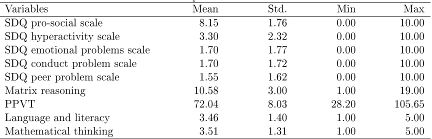
Table 1: Descriptive statistics of outcome variables
Variables Mean Std. Min Max
SDQ pro-social scale 8.15 1.76 0.00 10.00 SDQ hyperactivity scale 3.30 2.32 0.00 10.00 SDQ emotional problems scale 1.70 1.77 0.00 10.00 SDQ conduct problem scale 1.70 1.72 0.00 10.00 SDQ peer problem scale 1.55 1.62 0.00 10.00 Matrix reasoning 10.58 3.00 1.00 19.00
PPVT 72.04 8.03 28.20 105.65
Language and literacy 3.46 1.40 1.00 5.00 Mathematical thinking 3.51 1.31 1.00 5.00
ment. We use ve SDQ measures available in LSAC: 1) SDQ pro-social scale, (2) SDQ hyperactivity scale, (3) SDQ emotional problems scale, (4) SDQ conduct problems scale, and (5) SDQ peer problems. The SDQ pro-social scale was the sum of responses to ve 3-point questions (1=not true, 2=somewhat true, 3=certainly true) questions: 'considerate of other's feelings', 'readily share with children', 'helpful if someone is hurt', 'kind to younger children', and 'often volunteer to help'. Higher score for SDQ pro-social scale indicates a positive attitude. Similarly, SDQ hyper activity scale is the sum of re-sponses to ve 3-point questions: not been able to stay still, constantly dgeting, easily distracted, stopped to think before acting, and has a good attention span. Higher score for SDQ hyperactivity scale refers that the child is hyperactive. SDQ emotional problem scale was the sum of responses to 5 questions: 'complained of headache', 'often seemed worried', 'often been unhappy or tearful', 'nervous or easily lose condence', and 'had many fears'. Higher score of SDQ emotional problem scale indicates a emotional problem. In contrast, SDQ conduct problem scale was calculated as the mean of responses to ve 3-point Likert scale questions whether the child: 'has hot temper', 'not obedient, often ghts', 'argumentative with adults', and 'been spiteful to others'. The mean score was then rescaled to make an integer from 0 to 10. Similarly, the SDQ peer problem scale was calculated as the rescaled mean of responses to ve 3-point Likert scale questions: the child has been solitary, has no good friend, not liked by other children, bullied by children, and gets on better with adult. Higher score indicates a negative symptom except for SDQ pro-social scale, for which higher score indicates a positive outcome. Table 1 shows that children surveyed in LSAC achieved relatively good SDQ scores (i.e., high on pro-social scale and low on other SDQ scales).
All outcome variables examined in this study are collected from the responses of Parent 1, who is often the biological mother of the child. Children's behavioural outcome functions will be estimated by OLS in the rst stage, then random eects model will be used to account for unobserved heterogeneity. 4.2.2 Measures of Cognitive Outcomes
We will use the following measures of a child's cognitive development.
Matrix reasoning test (MR): Children from wave 2 to 4 completed the Matrix Reasoning (MR) test from the Wechsler Intelligence Scale for Children,4thedition (WISC-IV). MR test assessed a child's
The Peabody Picture Vocabulary Test (PPVT): The PPVT, which is only available in the rst three waves, was an interviewer-administered test that assessed a child's listening comprehension ability for spoken words in standard English. The PPVT test required a child to show the picture that best represented the meaning of a stimuli word spoken by the examiner (Dunn and Dunn, 1997). The sample of words were: sawing, wrapping, cage, exercising, fountain, nest, claw, delivering, frame and envelope.
Literacy and Mathematical skills were answered by both parents and teachers. We selected the results by teachers, assuming they had more detailed knowledge of the child's academic performance. For literacy skills, in Wave 1 this variable was the sum of yes answers to various yes/no questions about the child's experiment with writing tool, awareness of writing directionality, interest in copying, ability to write their names, simple words and simple sentences. From Wave 2 onwards, this variables consisted of the average of answers to a 5-point Likert scale questions, such as the child's contribution to classroom discussions, understanding and interpreting stories, reading and writing comprehension. Similarly, mathematical skills in Wave 1 was measured as the number of yes answers to questions such as ability to sort and count, recognition of numbers and do simple addition. From Wave 2 onwards, this variable captured the average of a series of 5-point Likert scale questions on issues such as understanding of place and value, organise data in graph, estimation of quantities, and use of various strategies to solve mathematical problems. We group the variables into ve point categorical order where higher values represent higher skills for mathematics and literacy. Table 1 shows that children covered in this survey achieved relatively high literacy, language skills and PPVT, on average.
4.3 Independent variables
the neighbourhood (parks, museum, trac safety), and stability and demographics (including the percentage of persons with high education and income) of neighbourhood.
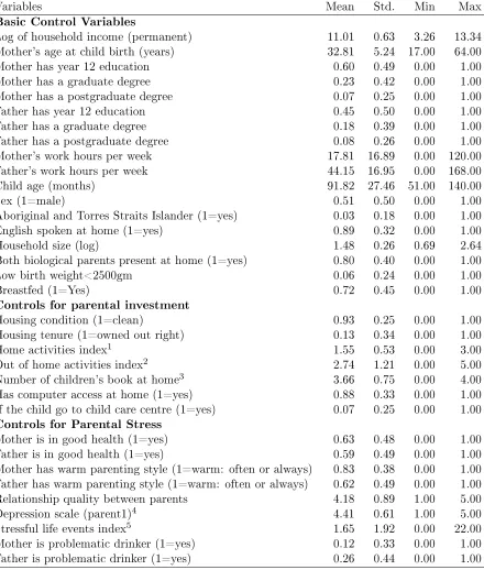
Table 2: Descriptive statistics: Independent variables
Variables Mean Std. Min Max
Basic Control Variables
Log of household income (permanent) 11.01 0.63 3.26 13.34 Mother's age at child birth (years) 32.81 5.24 17.00 64.00 Mother has year 12 education 0.60 0.49 0.00 1.00 Mother has a graduate degree 0.23 0.42 0.00 1.00 Mother has a postgraduate degree 0.07 0.25 0.00 1.00 Father has year 12 education 0.45 0.50 0.00 1.00 Father has a graduate degree 0.18 0.39 0.00 1.00 Father has a postgraduate degree 0.08 0.26 0.00 1.00 Mother's work hours per week 17.81 16.89 0.00 120.00 Father's work hours per week 44.15 16.95 0.00 168.00 Child age (months) 91.82 27.46 51.00 140.00 Sex (1=male) 0.51 0.50 0.00 1.00 Aboriginal and Torres Straits Islander (1=yes) 0.03 0.18 0.00 1.00 English spoken at home (1=yes) 0.89 0.32 0.00 1.00 Household size (log) 1.48 0.26 0.69 2.64 Both biological parents present at home (1=yes) 0.80 0.40 0.00 1.00 Low birth weight<2500gm 0.06 0.24 0.00 1.00 Breastfed (1=Yes) 0.72 0.45 0.00 1.00 Controls for parental investment
Housing condition (1=clean) 0.93 0.25 0.00 1.00 Housing tenure (1=owned out right) 0.13 0.34 0.00 1.00 Home activities index1 1.55 0.53 0.00 3.00
Out of home activities index2 2.74 1.21 0.00 5.00
Number of children's book at home3 3.66 0.75 0.00 4.00
Has computer access at home (1=yes) 0.88 0.33 0.00 1.00 If the child go to child care centre (1=yes) 0.07 0.25 0.00 1.00 Controls for Parental Stress
Mother is in good health (1=yes) 0.63 0.48 0.00 1.00 Father is in good health (1=yes) 0.59 0.49 0.00 1.00 Mother has warm parenting style (1=warm: often or always) 0.83 0.38 0.00 1.00 Father has warm parenting style (1=warm: often or always) 0.62 0.49 0.00 1.00 Relationship quality between parents 4.18 0.89 1.00 5.00 Depression scale (parent1)4 4.41 0.61 1.00 5.00
Stressful life events index5 1.65 1.92 0.00 22.00
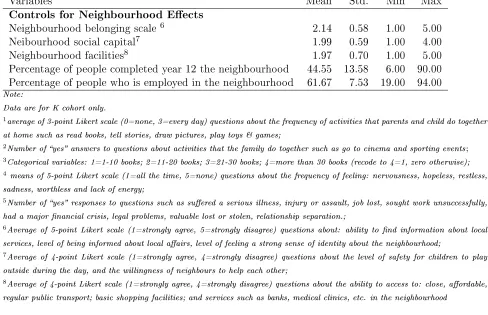
Table 2. Continued
Variables Mean Std. Min Max
Controls for Neighbourhood Eects
Neighbourhood belonging scale6 2.14 0.58 1.00 5.00
Neibourhood social capital7 1.99 0.59 1.00 4.00
Neighbourhood facilities8 1.97 0.70 1.00 5.00
Percentage of people completed year 12 the neighbourhood 44.55 13.58 6.00 90.00 Percentage of people who is employed in the neighbourhood 61.67 7.53 19.00 94.00
Note:
Data are for K cohort only.
1average of 3-point Likert scale (0=none, 3=every day) questions about the frequency of activities that parents and child do together
at home such as read books, tell stories, draw pictures, play toys & games;
2Number of yes answers to questions about activities that the family do together such as go to cinema and sporting events; 3Categorical variables: 1=1-10 books; 2=11-20 books; 3=21-30 books; 4=more than 30 books (recode to 4=1, zero otherwise);
4 means of 5-point Likert scale (1=all the time, 5=none) questions about the frequency of feeling: nervousness, hopeless, restless,
sadness, worthless and lack of energy;
5Number of yes responses to questions such as suered a serious illness, injury or assault, job lost, sought work unsuccessfully,
had a major nancial crisis, legal problems, valuable lost or stolen, relationship separation.;
6Average of 5-point Likert scale (1=strongly agree, 5=strongly disagree) questions about: ability to nd information about local
services, level of being informed about local aairs, level of feeling a strong sense of identity about the neighbourhood;
7Average of 4-point Likert scale (1=strongly agree, 4=strongly disagree) questions about the level of safety for children to play
outside during the day, and the willingness of neighbours to help each other;
8Average of 4-point Likert scale (1=strongly agree, 4=strongly disagree) questions about the ability to access to: close, aordable,
regular public transport; basic shopping facilities; and services such as banks, medical clinics, etc. in the neighbourhood
5 Results and discussions
To investigate the eects of family income on child outcomes, we rst use a basic set of controls (Specication 1). We then gradually include constructs for parental investments (Specication 2), family stress (Specication 3) and neighbourhood characteristics (Specication 4) in all regressions. Finally, we estimate a complete model (Specication 5) of child cognitive and non-cognitive development by including all controls from Specication 1 to Specication 5.
5.1 Cross-sectional estimates
In this section we estimate Equation9 to examine the relationship between parents' income and
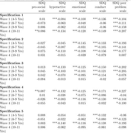
Table 3: Cross-sectional regressions: The eect of income on child non-cognitive development SDQ pro-social scale SDQ hyperactive scale SDQ emotional scale SDQ conduct scale SDQ peer problem scale Specication 1
Wave 1 (4-5 Yrs) 0.01 ***-0.084 ***-0.100 ***-0.136 ***-0.104 Wave 2 (6-7 Yrs) -0.073 -0.063 -0.048 -0.06 ***-0.111 Wave 3 (8-9 Yrs) 0.006 -0.062 -0.053 -0.06 ***-0.159 Wave 4 (10-11
Yrs) **0.086 ***-0.134 ***-0.120 ***-0.149 ***-0.207 Specication 2
Wave 1 (4-5 Yrs) -0.027 -0.045 ***-0.145 ***-0.133 ***-0.193 Wave 2 (6-7 Yrs) -0.045 *-0.087 -0.031 **-0.105 ***-0.141 Wave 3 (8-9 Yrs) 0.075 *-0.110 **-0.108 ***-0.156 ***-0.177 Wave 4 (10-11
Yrs) 0.031 -0.015 -0.039 *-0.079 0.007 Specication 3
Wave 1 (4-5 Yrs) 0.013 ***-0.133 ***-0.125 ***-0.150 ***-0.202 Wave 2 (6-7 Yrs) 0.045 **-0.103 **-0.101 ***-0.121 ***-0.205 Wave 3 (8-9 Yrs) 0.042 *-0.070 **-0.095 ***-0.154 *-0.078 Wave 4 (10-11
Yrs) -0.084 -0.013 0.015 -0.02 -0.057 Specication 4
Wave 1 (4-5 Yrs) **0.087 ***-0.132 ***-0.125 ***-0.171 ***-0.227 Wave 2 (6-7 Yrs) 0.01 -0.038 *-0.075 ***-0.086 -0.04 Wave 3 (8-9 Yrs) -0.026 **-0.083 ***-0.116 ***-0.130 ***-0.144 Wave 4 (10-11
Yrs) -0.055 -0.043 0.015 -0.032 *-0.100 Specication 5
Wave 1 (4-5 Yrs) 0.008 -0.054 -0.051 ***-0.132 -0.06 Wave 2 (6-7 Yrs) -0.051 -0.022 -0.062 *-0.080 ***-0.123 Wave 3 (8-9 Yrs) 0.003 ***-0.140 ***-0.116 ***-0.138 ***-0.193 Wave 4 (10-11
Yrs) 0.006 -0.062 -0.095 -0.061 -0.098
Note: Specication 1 includes basic set of covariates: log of household income, child's age, gender, birth weight, status of breastfeeding, education and hours of work of parents, age of mother at child birth and household size,English speaking household, and Aboriginal and Torres strait Islander.
Specication 2 includes Specication 1 plus indicators of parental investments: housing condition, housing tenure home activities index (frequency of someone engaging in activities (reading, drawing, and singing with the child), out of home activities index ( activities that the family do together such as go to cinema and sporting events), number of children's books at home,home computer use, and use of child care
Specication 3 Specication 1 plus indicators of family stress: parenting style, relationship between parents, frequency of stressful event, parental mental and physical health and whether parents are problematic drinkers.
Specication 4 includes covariates in Specication 1 plus neighbourhood characteristics: ), Neighbourhood belonging scale, Neighourhood social capital scale, Neighbourhood facilities,Percentage of people completed year 12 in the neighbourhood,Percentage of families earn <$1k/week in the neighbourhood, Percentage of people who is employed in the neighbourhood
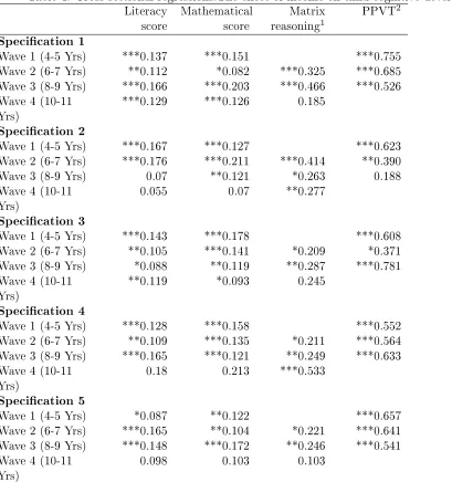
The results in Table 4 reveal that income is positively and signicantly associated with child cogni-tive development. Family income has a very signicant posicogni-tive eect on a child's cognicogni-tive development. The inclusion of a richer set of covariates (Specication 5) did not result in a less signicant association between income and cognitive measures except for Wave 4. Comparing Table 3 and 4, we see that the magnitude of the income parameter is higher for a child's cognitive development than it is for non-cognitive outcomes.
Table 4: Cross-sectional regressions:The eect of income on child cognitive development Literacy
score Mathematicalscore reasoningMatrix1
PPVT2
Specication 1
Wave 1 (4-5 Yrs) ***0.137 ***0.151 ***0.755 Wave 2 (6-7 Yrs) **0.112 *0.082 ***0.325 ***0.685 Wave 3 (8-9 Yrs) ***0.166 ***0.203 ***0.466 ***0.526 Wave 4 (10-11
Yrs) ***0.129 ***0.126 0.185 Specication 2
Wave 1 (4-5 Yrs) ***0.167 ***0.127 ***0.623 Wave 2 (6-7 Yrs) ***0.176 ***0.211 ***0.414 **0.390 Wave 3 (8-9 Yrs) 0.07 **0.121 *0.263 0.188 Wave 4 (10-11
Yrs) 0.055 0.07 **0.277 Specication 3
Wave 1 (4-5 Yrs) ***0.143 ***0.178 ***0.608 Wave 2 (6-7 Yrs) **0.105 ***0.141 *0.209 *0.371 Wave 3 (8-9 Yrs) *0.088 **0.119 **0.287 ***0.781 Wave 4 (10-11
Yrs) **0.119 *0.093 0.245 Specication 4
Wave 1 (4-5 Yrs) ***0.128 ***0.158 ***0.552 Wave 2 (6-7 Yrs) **0.109 ***0.135 *0.211 ***0.564 Wave 3 (8-9 Yrs) ***0.165 ***0.121 **0.249 ***0.633 Wave 4 (10-11
Yrs) 0.18 0.213 ***0.533 Specication 5
Wave 1 (4-5 Yrs) *0.087 **0.122 ***0.657 Wave 2 (6-7 Yrs) ***0.165 **0.104 *0.221 ***0.641 Wave 3 (8-9 Yrs) ***0.148 ***0.172 **0.246 ***0.541 Wave 4 (10-11
Yrs) 0.098 0.103 0.103
Note: Covariates of all specications are the same as in Table 2. Other covariates are skipped for brevity. Signicant levels are: ***=1%, **=5% and *=10%. 1Data is not available for Wave 1; 2Data is not available for Wave 4
5.2 Panel data estimates
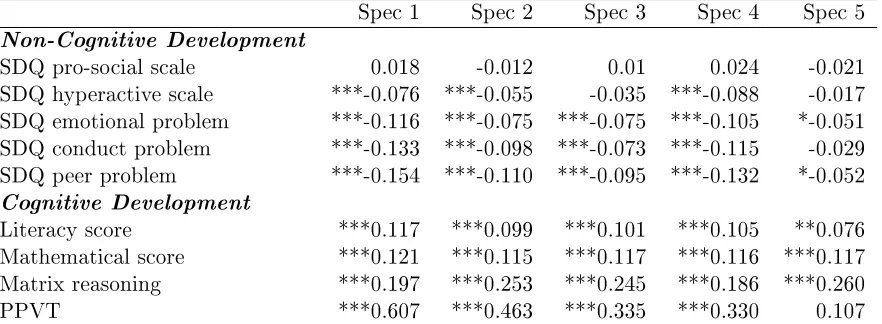
Table 5: Pooled regressions (static): The eect of income on child non-cognitive and cognitive devel-opment
Spec 1 Spec 2 Spec 3 Spec 4 Spec 5 Non-Cognitive Development
SDQ pro-social scale 0.018 -0.012 0.01 0.024 -0.021 SDQ hyperactive scale ***-0.076 ***-0.055 -0.035 ***-0.088 -0.017 SDQ emotional problem ***-0.116 ***-0.075 ***-0.075 ***-0.105 *-0.051 SDQ conduct problem ***-0.133 ***-0.098 ***-0.073 ***-0.115 -0.029 SDQ peer problem ***-0.154 ***-0.110 ***-0.095 ***-0.132 *-0.052 Cognitive Development
Literacy score ***0.117 ***0.099 ***0.101 ***0.105 **0.076 Mathematical score ***0.121 ***0.115 ***0.117 ***0.116 ***0.117 Matrix reasoning ***0.197 ***0.253 ***0.245 ***0.186 ***0.260 PPVT ***0.607 ***0.463 ***0.335 ***0.330 0.107
Note: Covariates of all specications are the same as in Table 2. Other covariates are skipped for brevity. Signicant levels are: ***=1%, **=5% and *=10%
aects cognitive and non-cognitive outcomes of children with the exception of the SDQ pro-social scale. In addition, the inclusion of additional covariates such as household's investment, family stress and neighbourhood characteristics separately to the basic set of controls (Specication 2, 3 and 4) did not aect the signicance level of the income parameter. However, when all these additional covariates are used (i.e, Specication 5), the fewer non-cognitive outcomes are signicantly associated with household income. This suggests that when we consider the eects of income on child development in a broader context there are some specic variables in these four Specications which are responsible for mediating the eects of income on child non-cognitive development. Surprisingly the eects of family income on child cognitive development remained consistently signicant even in Specication 5, with the exception of PPVT.
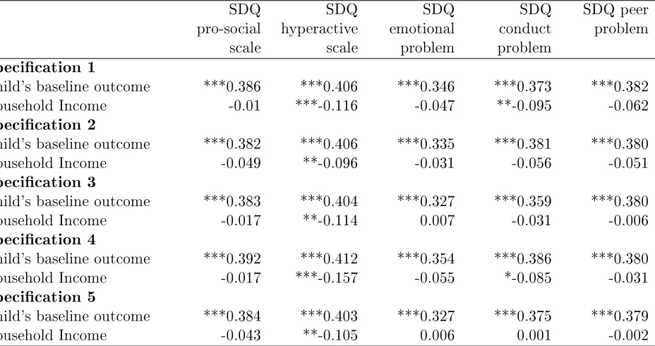
are consistently statistically signicant across all regressions. Household income does not signicantly determine the child's SDQ pro-social skill, which is consistent with the ndings from cross-sectional and pooled regressions. The income parameter still has the expected negative sign for the remaining non-cognitive measures but the statistical signicance is no longer achieved for the SDQ emotional problem scale and the SDQ peer problem scale. In addition, the magnitude of the income parameter reduces considerably compared to the cross-sectional estimates. However, these results reveal a causual relationship between family income and child's SDQ hyperactivity scale in that children from low income family are more likely to be hyperactive.
Table 6: Dynamic panel data model: The eect of income on child non-cognitive behaviour (Random eects model)
SDQ pro-social scale
SDQ hyperactive scale
SDQ emotional problem
SDQ conduct problem
SDQ peer problem
Specication 1
Child's baseline outcome ***0.386 ***0.406 ***0.346 ***0.373 ***0.382 Household Income -0.01 ***-0.116 -0.047 **-0.095 -0.062 Specication 2
Child's baseline outcome ***0.382 ***0.406 ***0.335 ***0.381 ***0.380 Household Income -0.049 **-0.096 -0.031 -0.056 -0.051 Specication 3
Child's baseline outcome ***0.383 ***0.404 ***0.327 ***0.359 ***0.380 Household Income -0.017 **-0.114 0.007 -0.031 -0.006 Specication 4
Child's baseline outcome ***0.392 ***0.412 ***0.354 ***0.386 ***0.380 Household Income -0.017 ***-0.157 -0.055 *-0.085 -0.031 Specication 5
Child's baseline outcome ***0.384 ***0.403 ***0.327 ***0.375 ***0.379 Household Income -0.043 **-0.105 0.006 0.001 -0.002
Note: Specications are the same as in Table 2. Other covariates are skipped for brevity. Signicant levels are: ***=1%, **=5% and *=10%
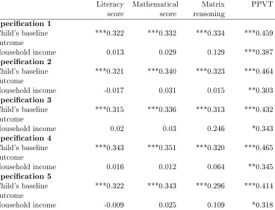
Table 7: Dynamic panel data model: The eect of income on child cognitive behaviour(Random eects model
Literacy
score Mathematicalscore reasoningMatrix PPVT Specication 1
Child's baseline
outcome ***0.322 ***0.332 ***0.334 ***0.459 Household income 0.013 0.029 0.129 ***0.387 Specication 2
Child's baseline
outcome ***0.321 ***0.340 ***0.323 ***0.464 Household income -0.017 0.031 0.015 **0.303 Specication 3
Child's baseline
outcome ***0.315 ***0.336 ***0.313 ***0.432 Household income 0.02 0.03 0.246 *0.343 Specication 4
Child's baseline
outcome ***0.343 ***0.351 ***0.320 ***0.465 Household income 0.016 0.012 0.064 **0.345 Specication 5
Child's baseline
outcome ***0.322 ***0.343 ***0.296 ***0.414 Household income -0.009 0.025 0.109 *0.318
Note: Covariates of all specications are the same as in Table 2. Other covariates are skipped for brevity. Signicant levels are: ***=1%, **=5% and *=10%
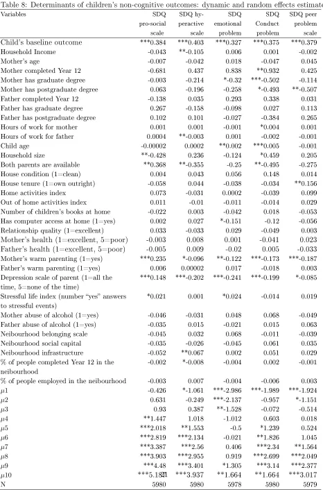
6 Factors mediating the eects of income
are less likly to have behavioural problems.
Table 8: Determinants of children's non-cognitive outcomes: dynamic and random eects estimates Variables SDQ pro-social scale SDQ hy-peractive scale SDQ emotional problem SDQ Conduct problem SDQ peer problem scale
Child's baseline outcome ***0.384 ***0.403 ***0.327 ***0.375 ***0.379
Household Income -0.043 **-0.105 0.006 0.001 -0.002
Mother's age -0.007 -0.042 0.018 -0.047 0.045
Mother completed Year 12 -0.681 0.437 0.838 **0.932 0.425
Mother has graduate degree -0.003 -0.214 *-0.32 ***-0.502 -0.114
Mother has postgraduate degree 0.063 -0.196 -0.258 *-0.493 **-0.507
Father completed Year 12 -0.138 0.035 0.293 0.338 0.031
Father has graduate degree 0.267 -0.158 -0.098 0.027 0.113
Father has postgraduate degree 0.102 0.101 -0.027 -0.384 0.265
Hours of work for mother 0.001 0.001 -0.001 *0.004 0.001
Hours of work for father 0.0004 **-0.003 0.001 -0.002 -0.001
Child age -0.00002 0.0002 **0.002 ***0.005 -0.001
Household size **-0.428 0.236 -0.124 *0.459 0.205
Both parents are available **0.368 **-0.355 -0.25 **-0.495 -0.275
House condition (1=clean) 0.004 0.043 0.056 0.148 0.014
House tenure (1=own outright) -0.058 0.044 -0.038 -0.034 **0.156
Home activities index 0.073 -0.031 0.0002 -0.039 0.099
Out of home activities index 0.011 -0.01 -0.011 -0.014 0.029
Number of children's books at home -0.022 0.003 -0.042 0.018 -0.053
Has computer access at home (1=yes) 0.002 0.027 *-0.151 -0.12 -0.056
Relationship quality (1=excellent) 0.033 -0.033 0.029 -0.049 0.003
Mother's health (1=excellent, 5=poor) -0.003 0.008 0.001 -0.041 0.023 Father's health (1=excellent, 5=poor) -0.005 0.009 -0.02 0.005 -0.033
Mother's warm parenting (1=yes) ***0.235 *-0.096 **-0.122 ***-0.173 ***-0.187
Father's warm parenting (1=yes) 0.006 0.00002 0.017 -0.018 0.003
Depression scale of parent (1=all the time, 5=none of the time)
***0.148 ***-0.202 ***-0.241 ***-0.199 *-0.085
Stressful life index (number yes answers to stressful events)
*0.021 0.001 *0.024 -0.014 0.019
Mother abuse of alcohol (1=yes) -0.046 -0.031 0.048 0.068 -0.049
Father abuse of alcohol (1=yes) -0.035 0.015 -0.021 0.015 0.063
Neibourhood belonging scale -0.045 0.032 0.068 -0.011 -0.039
Neibourhood social capital -0.035 -0.026 -0.045 0.061 0.035
Neibourhood infrastructure -0.052 **0.067 0.002 0.051 0.029
% of people completed Year 12 in the neibourhood
-0.002 *-0.008 -0.004 0.002 -0.001
% of people employed in the neibourhood -0.003 0.007 -0.004 -0.006 0.003
µ1 -0.426 *-1.061 ***-2.986 ***-1.989 ***-1.924
µ2 0.631 -0.249 ***-2.137 -0.957 *-1.151
µ3 0.93 0.387 **-1.528 -0.072 -0.514
µ4 **1.447 1.018 -1.012 0.603 0.018
µ5 ***2.018 **1.553 -0.5 *1.239 0.524
µ6 ***2.819 ***2.134 -0.021 **1.826 1.045
µ7 ***3.387 ***2.56 0.406 ***2.34 **1.564
µ8 ***3.903 ***2.955 0.919 ***2.699 ***2.049
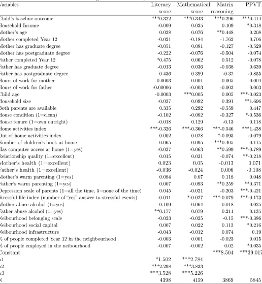
Table 9: Determinants of children's cognitive outcomes: dynamic and random eects estimates
Variables Literacy
score Mathematicalscore reasoningMatrix PPVT
Child's baseline outcome ***0.322 ***0.343 ***0.296 ***0.414
Household Income -0.009 0.025 0.109 *0.318
Mother's age 0.028 0.076 **0.448 0.208
Mother completed Year 12 -0.021 -0.184 -1.762 0.706
Mother has graduate degree -0.051 0.081 -0.127 -0.529
Mother has postgraduate degree -0.222 -0.076 -0.504 -0.074
Father completed Year 12 *0.475 0.062 0.512 -0.078
Father has graduate degree -0.013 0.036 -0.038 0.639
Father has postgraduate degree 0.436 0.399 -0.32 -0.855
Hours of work for mother -0.0003 0.001 -0.005 0.004
Hours of work for father -0.00006 -0.003 -0.003 0.003
Child age -0.0003 ***0.005 0.005 ***-0.023
Household size -0.037 0.092 0.391 **1.696
Both parents are available 0.335 0.292 -0.559 0.447
House condition (1=clean) -0.102 -0.082 -0.327 *-0.536
House tenure (1=own outright) -0.018 0.129 -0.13 0.118
Home activities index ***-0.326 ***-0.366 ***-0.546 ***1.438
Out of home activities index 0.002 0.028 *-0.095 -0.079
Number of children's book at home 0.065 0.095 ***0.405 0.115
Has computer access at home (1=yes) -0.037 -0.063 **0.599 ***-0.789
Relationship quality (1=excellent) 0.015 0.031 -0.074 **-0.218
Mother's health (1=excellent) 0.023 0.05 -0.013 0.071 Father's health (1=excellent) -0.036 -0.024 0.006 -0.108
Mother's warm parenting (1=yes) 0.084 0.07 0.118 0.048
Father's warm parenting (1=yes) 0.007 -0.093 **0.259 **0.371
Depression scale of parents (1=all the time, 5=none of the time) 0.045 -0.021 -0.203 ***-0.421 Stressful life index (number of yes answer to stressful events) -0.011 *-0.027 ***-0.079 ***-0.173
Mother abuse alcohol (1=yes) -0.109 -0.064 -0.018 0.025
Father abuse alcohol (1=yes) **0.177 0.079 0.211 0.135
Neibourhood belonging scale -0.023 -0.025 -0.15 ***-0.386
Neibourhood social capital 0.007 0.022 0.113 *0.216
Neibourhood infrastructure -0.043 -0.012 0.074 0.19
% of people completed Year 12 in the neighbourhood -0.003 0.001 -0.023 0.015
% of people employed in the neibourhood -0.007 -0.002 0.02 *0.035
Constant ***8.504 ***39.017
µ1 *1.502 ***2.784
µ2 ***2.298 ***3.833
µ3 ***3.528 ***5.226
N 4398 4159 3869 5845
7 Conclusions
non-cognitive outcomes that have rarely been explored in the Australian context. Second, it examines the association between household income and child outcomes both in cross section using a `mopping-up' approach and in the longitudinal dimension using random eects approaches to account the potential endogeneity of income and unobserved individual heterogeneity. Third, it investigates whether the relationship between child outcomes and income can be mediated by `parental investment', `parental stress' and 'neighbourhood characteristics'.
Our results show that, when individual unobserved eect is not controlled for, income has signicant eects on behavioural outcomes of children with the exception of the SDQ pro-social scale. However, when unobserved heterogeneity is controlled using a richer set of covariates and random eects model, the eect of income on children's non-cognitive outcomes becomes insignicant, except for SDQ hyper-activity scale. For cognitive outcomes, when a rich set of controls is used, income remains signicantly associated with child outcomes. However, when individual unobserved eect is controlled for using a random eects estimator, income is no longer a signicant determinant of children's cognitive outcome (except for PPVT scores, which is signicant at only 10%). Our results provide some causal relation-ship between parental socio-economic status and child behavioural development. We nd that children from low income households are more likely to be hyperactive and children of highly educated mother are less likely to have conduct problems. Children from a household, where both biological parents live together, are less likely to have behavioural problems. This paper, however, reveals a rather moderate relationship between child development and family income, and a strong eect on child outcomes of parental characteristics such as parenting style and parental mental health.
References
Alderson, D., Gennetian, L., Dowsett, C., Imes, A., and Huston, A. (2008). Eects of employment-based programs on families by prior levels of disadvantage. Social Service Review.
Aughinbaugh, A. and Gittleman, M. (2003). Does money matter? Journal of Human Resources, 38(2):416440.
Baetschmann, G., Staub, K. E., and Winkelmann, R. (2011). Consistent estimation of the xed eects ordered logit model. Technical report, Institute for the Study of Labor (IZA), University of Zurich, No. 5443.
Becker, G. (1981). A Treatise on the Family. Harvard Univ Press.
Becker, G. and Lewis, G. (1973). On the interaction between the quantity and quality of children. The Journal of Political Economy, 81:S279S288.
Becker, G. and Tomes, N. (1986). Human capital and the rise and fall of families. Journal of Labor Economics, 4:S1S39.
Blau, D. (1999a). The eect of child care characteristics on child development. Journal of Human Resources, pages 786822.
Blau, D. (1999b). The eect of income on child development. Review of Economics and Statistics, 81(2):261276.
Bradshaw, J., Hoelscher, P., and Richardson, D. (2007). An index of child well-being in the european union. Social Indicators Research, 80:133177.
Brooks-Gunn, J. and Duncan, G. (1997). The eects of poverty on children. The future of children, pages 5571.
Carro, J. (2007). Estimating dynamics panel data discrete choice model models with xed eects. Journal of Econometrics, 140(2):503528.
Case, A., Lubotsky, D., and Paxson, C. (2002). Economic status and health in childhood: The origins of the gradient. The American Economic Review, 92(5):13081344.
Chamberlain, G. (1980). Analysis of covariance with qualitative data. Review of Economic Studies, 47:225238.
Contoyannis, P., Jones, A., and Rice, N. (2004). The dynamics of health in the british household panel survey. Journal of Applied Econometrics, 19(4):473503.
Contoyannis, P. and Li, J. (2011). The evolution of health outcomes from childhood to adolescence. Journal of Health Economics, 30:1132.
Cunha, F. and Heckman, J. (2007). The technology of skill formation. American Economic Review, 97:3147.
Cunha, F., Heckman, J., and Schennach, S. (2010). Estimating the technology of cognitive and noncog-nitive skill formation. Econometrica, 78(3):883931.
Currie, A., Shields, M. A., and Price, S. W. (2007). The child health/family income gradient: Evidence from england. Journal of Health Economics, 26(2):213232.
Currie, J. (2009). Healthy, wealthy, and wise: Socio-economic status, poor health in childhood, and human capital development. Journal of Economic Literature, 47:87122.
Currie, J. and Stabile, M. (2003). Socioeconomic status and child health: Why is the relationship stronger for older children. The American Economic Review, 93(5):18131823.
Dahl, G. and Lochner, L. (2005). The impact of family income on child achievement. Technical report, National Bureau of Economic Research.
Dearing, E., Kreider, H., Simpkins, S., and Weiss, H. (2006). Family involvement in school and low-income children's literacy: Longitudinal associations between and within families. Journal of Educational Psychology, 98(4):653.
Dooley, M. and Stewart, J. (2007). Family income, parenting styles and child behaviouralemotional outcomes. Health economics, 16(2):145162.
Duncan, G., Yeung, W., Brooks-Gunn, J., and Smith, J. (1998). How much does childhood poverty aect the life chances of children? American Sociological Review, pages 406423.
Dunn, L. M. and Dunn, L. M. (1997). Peabody Picture Vocabulary Test (3rd Ed.). Circle Pines, MN: American Guidance Service.
Ferrer-i Carbonell, A. and Frijters, P. (2004). How important is methodology for the estimate of the determinants of hapiness? The Economic Journal, 114:641659.
Gornick, J. and Jäntti, M. (2010). Child poverty in upper-income countries: Lessons from the luxem-bourg income study. From Child Welfare to Child Well-Being, pages 339368.
Gregg, P., Washbrook, E., Propper, C., and Burgess, S. (2005). The eects of a mother's return to work decision on child development in the uk. Economic Journal, 115(501):F48 F80.
Guo, G. and Harris, K. (2000). The mechanisms mediating the eects of poverty on children's intellec-tual development. Demography, 37(4):431447.
Heckman, J. (2007). The economics, technology, and neuroscience of human capability formation. Proceedings of the National Academy of Sciences, 104(33):1325013255.
Khanam, R., Nghiem, H. S., and Connelly, L. B. (2009). Child health and the income gradient: evidence from australia. J Health Econ, 28(4):805817.
Maurin, E. (2002). The impact of parental income on early schooling transitions:: A re-examination using data over three generations. Journal of Public Economics, 85(3):301332.
Mayer, S. (1997). What money can't buy: Family income and children's life chances. Harvard Univ Pr.
Morris, P., Duncan, G., and Rodriguez, C. (2004). Using welfare reform experiments to estimate the impact of income on child achievement. Unpublished manuscript, Northwestern University.
Mundlak, Y. (1978). On the pooling of time series and cross section data. Econometrica, 46:6985.
Pebley, A. and Sastry, N. (2004). Neighborhoods, poverty, and children's well-being. Social inequality, pages 119145.
Rosenzweig, M. R. and Schultz, T. P. (1983). Estimating a household production function: Hetero-geneity, the demand for health inputs, and their eects on birth weight. The Journal of Political Economy, 91(5):723746.
Rosenzweig, M. R. and Wolpin, K. I. (1988). Heterogeneity, intrafamily distribution, and child health. The Journal of Human Resources, 23(4):437461.
Shea, J. (2000). Does parents' money matter? Journal of Public Economics, 77(2):155 184.
Smith, J. and Brooks-Gunn, J. (1997). Correlates and consequences of harsh discipline for young children. Archives of Pediatrics and Adolescent Medicine, 151(8):777.
Violato, M., Petrou, S., Gray, R., and Redshaw, M. (2010). Family income and child cognitive and behavioural development in the united kingdom: does money matter? Health Economics.
Yamauchi, C. (2010). Parental investment in children: Dierential pathways of parental education and mental health*. Economic Record, 86(273):210226.