Theses Thesis/Dissertation Collections
4-24-2013
Determining a substitution matrix for the
alignment of disordered proteins
Dong Kim
Follow this and additional works at:http://scholarworks.rit.edu/theses
This Thesis is brought to you for free and open access by the Thesis/Dissertation Collections at RIT Scholar Works. It has been accepted for inclusion in Theses by an authorized administrator of RIT Scholar Works. For more information, please [email protected].
Recommended Citation
R∙I∙T
Determining a substitution matrix for the
alignment of disordered proteins
by
Dong Jin Kim
Submitted in partial fulfillment of the requirements for the Master of Science
degree in Bioinformatics at Rochester Institute of Technology
Thomas H. Gosnell School of Life Science
College of Science
Rochester Institute of Technology
Rochester, NY
Committee Approval:
______________________________________________________________________________
Michael V. Osier, Ph.D. Date
Thesis Advisor
______________________________________________________________________________
Gary R. Skuse, Ph.D. Date
Committee Member
______________________________________________________________________________
Gregory A. Babbitt, Ph.D. Date
Abstract
As the research of disordered proteins progresses and more disordered protein sequences
are discovered, an optimal substitution matrix for the alignment of these sequences must be
elucidated. The currently used substitution matrices, PAM and BLOSUM, are ideal for the
alignment of general protein sequences. But it is discovered that this set of matrices is not
adequate for the specific alignment of disordered protein sequences. By implementing genetic
algorithms, a substitution matrix improved for the alignment of disordered proteins has been
achieved. The genetic algorithm determined matrix performed two times better when compared
to BLOSUM62 and PAM250.
Introduction
The traditional belief is that the primary requirement for a protein to function properly is
that it needs to fold into a tightly ordered three dimensional structure [1]. But there have been
many studies to show that this is not always the case. There are whole proteins or regions of
proteins that do not fold spontaneously into a well-organized globular structure. These proteins
are called intrinsically disordered [2]. Intrinsic disorder is found in a variety of proteins and
although they lack a tightly ordered three dimensional structure, they carry out many different
complex functions [1-4]. As the study of disordered proteins advances, accurate sequence
alignments of these proteins will be necessary in research areas such as molecular evolutionary
studies, homology modeling, and protein function studies. In molecular evolutionary studies,
inaccurate sequence alignments could potentially cause the construction of an erroneous
phylogenic tree. This can ultimately lead to an incorrect analysis of the evolutionary relationship
shared by the proteins being studied. In homology modeling, a more accurate sequence
alignment will yield a more accurate identification of structural motifs when the three
dimensional structure of the protein is unknown. A more accurate identification of structural
motifs can also aid in protein function prediction of that same unknown protein.
The two prominently used substitution matrices for sequence alignment are the Blocks of
Amino Acid Substitution Matrix (BLOSUM) and Point Accepted Mutation (PAM) matrices.
The BLOSUM set of matrices was constructed using blocks of highly conserved regions while
the PAM matrix was constructed using global alignments of highly similar, closely related
based on the frequency of the substitution being observed. Both matrices were created using a
wide variety of protein families [5, 6]. Therefore, both matrices work well for an overall
generalized set of proteins, but are not specific for the alignment of disordered proteins.
It has been shown that the order and disorder of protein regions is determined by their
amino acid composition [7]. Disordered proteins are also characterized by low-sequence
complexity [8]. Since disordered proteins are known to lack tightly ordered structure it would be
reasonable to assume that they would have amino acid compositions which are strictly
hydrophobic. But it has been found that disordered proteins are composed of both hydrophilic
and hydrophobic amino acids. More specifically, disordered proteins have a propensity for A, R,
G, Q, S, P, E and K with a decrease of W, C, F, I, Y, V, L and N. The amino acids H, M, T, and
D are consistent in ordered and disordered regions [9]. It has also been shown that disordered
protein regions have a higher evolutionary rate or change when compared to ordered regions of
proteins [10]. The predisposition of disordered proteins for a specific set of amino acids along
with a higher evolutionary rate give sufficient evidence that the frequency of observed mutations
will be different that those reflected by both BLOSUM and PAM matrices. Therefore the
BLOSUM and PAM set of matrices are not suitable for the best alignment of disordered regions
or disordered whole proteins. Therefore we propose a new substitution matrix which better
reflects the observed frequency of mutation within disordered protein regions and disordered
whole proteins.
Intrinsically disordered proteins or regions can be identified experimentally through
X-ray crystallography, NMR spectroscopy, circular dichroism (CD) spectroscopy, protease
digestion, Stoke’s radius determination, or any combination of methods to verify disorder [11].
There exists a curated database of disordered proteins, Disprot, where disordered proteins were
found experimentally using the above methods [12]. Currently there are 684 proteins with 1513
disordered regions in the database (www.disprot.org). Although the database is growing, not all
disordered proteins are documented. If your protein of interest is not found in the database there
are other resources to identify disorder. There are predictors of disordered regions such as
DisEMBL, DISOPRED2, IUPred, and PONDR just to name a few. The listed predictors are
overall fairly accurate but with any predictor, the results are not always completely accurate [8,
13-15]. A predictor can potentially give false positives, allowing parts of the ordered protein
protein sequences. Taking advantage of a curated database of experimentally determined
disordered protein sequences would be more advantageous than using sequences based on a
predictor. In order to produce a precise substitution matrix for the alignment of disordered
proteins, the Disprot database sequences will be used in training the genetic algorithm rather than
using sequences collected by predictors.
Utilizing the sequence data found in the Disprot database, the creation of a new
substitution matrix for disordered proteins was performed. The disordered protein sequences
were used to create training and testing data sets which were fed into a genetic algorithm (GA).
A genetic algorithm mimics what is seen in real world genetics by using crossover, mutation and
selection [16]. Selection is based on the fitness score where a higher score means it is more fit
therefore has a higher chance of being selected for mating. For the purpose of finding the best
scoring matrix, the matrix’s fitness will be determined by how well it can align disordered
proteins. After a series of crossovers and mutations, the evolutionary pressure of the GA to
better align disordered proteins forces the matrices to slowly develop into a more appropriate
matrix. Our focus is to produce a substitution matrix that is better optimized for the alignment of
disordered proteins.
Materials and Methods
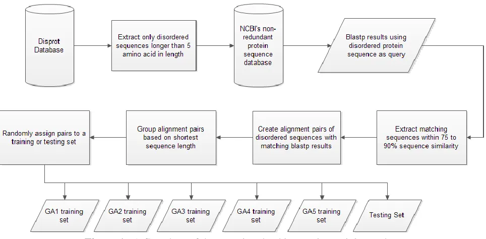
Creating the training and testing data set
The disordered protein sequences were downloaded from the Disprot database and only
the portions of the whole protein sequences which were identified as being disordered were
collected. Any sequence less than five amino acids in length were rejected. The disordered
sequences from the Disprot database were then used to accumulate homologous sequences to
create large enough training and testing sets to be used in the genetic algorithm. Using the
NCBI’s non-redundant protein sequences (nr) database, a blastp search was performed using all
of the disordered sequences extracted from Disprot as the query sequence. Only sequences
within the range of 75-90% similarity to the query sequence were filtered and kept. It was
assumed the disordered sequences from the Disprot database would align to the disordered
Figure 1. A flowchart of the steps involved in creating training and testing sets containing disordered protein sequences from the Disprot database and NCBI’s non-redundant protein sequence database.
Sequence alignment pairs were then created by pairing the Disprot sequence with the
matching blast search result. The alignment pairs were then sorted by sequence length based on
the shortest amino acid length member of the pair. The sorted sequences were then distributed
evenly and randomly into six different groups. Five of the six were used as the training sets in
five separate GA runs. The last group was saved for testing the resulting GA determined scoring
matrices against currently used scoring matrices for the alignment of proteins. The overall
process of creating the training and testing sets is diagramed in figure 1.
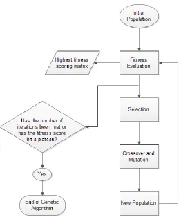
Running the genetic algorithm (GA)
The Genetic Algorithm is a cyclic three step process first initialized with a starting
population of individuals. An individual is defined as the scoring matrix along with
corresponding gap-open and gap-extend scores. After the initial population has been set, the
next steps of the GA are a fitness evaluation of the population, selection for mating, and
crossover and mutation, which are repeated until the genetic algorithm converges to a solution.
Figure 2. A diagram of the Genetic Algorithm process.
The initial population contained a wide range of the PAM set of matrices which included
the PAM10 to PAM500 set of matrices. Each matrix had every possible combination of the
corresponding gap-opening score ranging from 1 to 14 in 0.5 increments and a gap-extending
scores in 0.5 to 2 in 0.5 increments, where the opening score must be greater than the
gap-extending score. The ranges of gap penalties were used by Radivojac et al. in their study to
improve sequence alignments of intrinsically disordered proteins [17]. The matrices were
downloaded from NCBI’s FTP site (ftp://ftp.ncbi.nih.gov/blast/matrices/). The matrices with
corresponding gap-open and gap-extend scores were then evaluated for fitness.
The first step in the cyclic process of the genetic algorithm is the fitness evaluation. The
fitness of each matrix was determined by the sum of all the alignment scores calculated by the
alignment of all pairs of sequences in the training set as described previously. The sequence
alignment JAVA API, JAligner (http://jaligner.sourceforge.net/) was used to calculate alignment
scores given the scoring matrix along with the corresponding gap scores and the sequence pairs
alignments while a less fit individual will have a lower score due to poor alignments. Once all
the individual’s fitness scores were calculated, selection for mating followed.
Selection for mating, the second step of the cyclic process, was performed in order to
determine the parents for mating, thus creating the next generation of individuals. Selection was
based on the fitness of the individual. The more fit an individual, the more likely it will pass part
of its scoring matrices and gap scores onto the next generation. Selection for mating was
performed by first sorting the current population based on its fitness scores from greatest to
lowest. Then, random numbers were generated following a beta distribution using alpha and
beta values of 0.5 and 2 respectively. The random number generated chose the rank number and
ultimately the individual for mating. As a result, the higher ranked individual had a higher
[image:9.612.74.530.301.454.2]probability of mating while lower ranked individuals had a lower probability of mating.
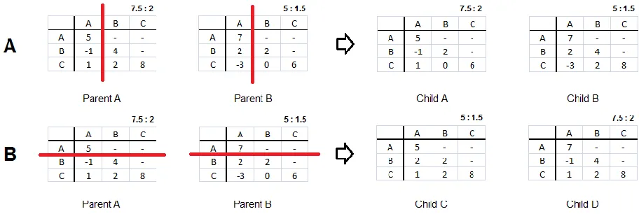
Figure 3. The crossover of Parent A with Parent B yields the children shown. The red line indicates the randomly selected point of crossover. The set of numbers above the matrix is the gap-opening and gap-extended penalties. Figure 3A shows a column crossover of Parent A with Parent B to produce Child A and Child B. Figure 3B illustrates a row crossover.
The third cyclic step of the GA is the crossover and mutation of the matrices of the
chosen individuals for mating. When a pair of individuals is selected for mating, the two
matrices or “Parents,” will be crossed over at randomly selected columns or rows to produce two
matrices or “Children” for the next generation. The crossover and mutation of the matrices is
illustrated in Figure 3. The resulting matrices have the associated opening and
gap-extending score of the parent who has the most influence in producing the child. For example, in
figure 3B, Child C is given the gap penalties of Parent B because the majority of the matrix has
numbers of crossover points were tested and it was found that two crossover points produced the
greatest diversity in the population. Therefore two crossover points were used for all GA runs.
In order to prevent all of the scores of the matrices to be artificially inflated, there must
be a rule in place so that the entire matrix does not simply become a matrix of high positive
numbers. Therefore the matrices were converted to mutation probability matrices after
crossover. Because the matrix is represented by probably values, the columns of the matrix must
add up to 1. This rule inhibited the values of the matrices from becoming inflated. The
individual’s matrix was converted to its mutation probability matrix by manipulating the same
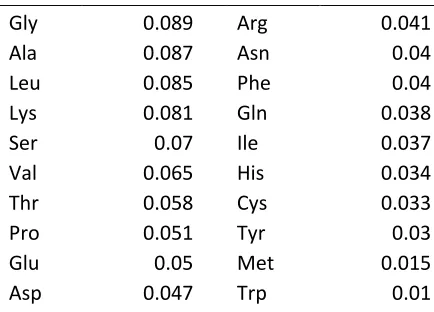
log odds formula used by Dayhoff shown below.
The variable PAMij is the score seen in the PAM matrix for the substitution of amino acid i to
amino acid j. The variable Mij is the probability of amino acid i mutating to amino acid j and fi is
the normalized frequency of the amino acid. Formula A is the original log odds formula and
formula B is the algebraic manipulation of formula A to give the equation used to calculate the
mutation probability. Since the PAMij values can be extracted from the matrix in question, the
only variable needed is the frequency of the amino acid, fi. The fi values used was the
normalized frequency of the amino acid calculated by Dayhoff to produce the PAM set of
Table 1. The normalized frequencies of amino acids observed by Dayhoff to produce the PAM set of matrices.
Normalized Frequencies of the Amino Acids in the Accepted Point Mutation Data
Gly 0.089 Arg 0.041
Ala 0.087 Asn 0.04
Leu 0.085 Phe 0.04
Lys 0.081 Gln 0.038
Ser 0.07 Ile 0.037
Val 0.065 His 0.034
Thr 0.058 Cys 0.033
Pro 0.051 Tyr 0.03
Glu 0.05 Met 0.015
Asp 0.047 Trp 0.01
Once the matrix was represented as a mutation probability, random mutation of the
matrix can occur. If the individual has been chosen for mutation, a random point in the matrix is
chosen. That random point is then replaced by a randomly generated decimal number ranging
from 0 to 1. After the crossover and mutation steps, each column of the matrix was normalized
by the total value of the column allowing all the columns’ values to add to 1. Once the matrix
has been normalized, it was converted back to the scoring matrix using the same log-odds
formula seen in figure 4A and rounded to the nearest whole number. In order for the matrix to
be symmetrical, the average of the two substitution scores was calculated and applied.
After the new generation of individuals was created by mating the previous generation,
the cyclic process of the genetic algorithm was repeated. After each generation, the highest
fitness scoring matrix was saved along with its fitness score. The process was repeated until it
was observed that the fitness score reached a plateau. Each generation was limited to a
maximum population of 200. A pass-through parameter was also implemented in the genetic
algorithm, where a percentage of the top fitness ranking individuals were passed through to the
next generation. A pass-through rate of 1% along with the mutation rate of 10% was used for all
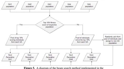
runs of the genetic algorithm. A beam search method was implemented after the 1000th generation had been reached and for every 500th generation thereafter. The beam search was executed by taking the top 10% of the population of every GA runs and grouping them together.
GA populations were filled by randomly choosing individuals from the pooled group that were
[image:12.612.71.544.111.376.2]not chosen as the top 10%. The overall beam search algorithm is diagramed in figure 5.
Figure 5. A diagram of the beam search method implemented in the genetic algorithm runs.
Comparing the GA determined substitution matrix to others
The genetic algorithm determined substitution matrix was compared to commonly used
substitution matrices. The matrices were compared by how well they can align disordered
protein sequences through the cumulative score they received by the alignment of disordered
sequences contained in the testing set. Although the GA determined matrix does provide optimal
gap scores, the other commonly used matrices do not. Therefore the highest cumulative
alignment score resulting from all the possible combinations of gap-opening values ranging from
1 to 14 in 0.5 increments with gap-extending values from 0.5 to 2 in 0.5 increments was used for
comparison. The most commonly used substitution matrices for protein sequence alignments,
BLOSUM50, BLOSUM63, BLOSUM80, PAM40, PAM80, PAM120, PAM250 and PAM350
were compared to the genetic algorithm determined matrix.
Results
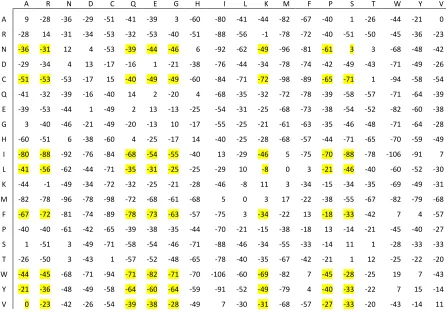
The GA determined disordered protein substitution matrix
matrix that all five GAs produced for the optimized alignment of disordered proteins is seen
shown in figure 6.
A R N D C Q E G H I L K M F P S T W Y V
A 9 -28 -36 -29 -51 -41 -39 3 -60 -80 -41 -44 -82 -67 -40 1 -26 -44 -21 0
R -28 14 -31 -34 -53 -32 -53 -40 -51 -88 -56 -1 -78 -72 -40 -51 -50 -45 -36 -23
N -36 -31 12 4 -53 -39 -44 -46 6 -92 -62 -49 -96 -81 -61 3 3 -68 -48 -42
D -29 -34 4 13 -17 -16 1 -21 -38 -76 -44 -34 -78 -74 -42 -49 -43 -71 -49 -26
C -51 -53 -53 -17 15 -40 -49 -49 -60 -84 -71 -72 -98 -89 -65 -71 1 -94 -58 -54
Q -41 -32 -39 -16 -40 14 2 -20 4 -68 -35 -32 -72 -78 -39 -58 -57 -71 -64 -39
E -39 -53 -44 1 -49 2 13 -13 -25 -54 -31 -25 -68 -73 -38 -54 -52 -82 -60 -38
G 3 -40 -46 -21 -49 -20 -13 10 -17 -55 -25 -21 -61 -63 -35 -46 -48 -71 -64 -28
H -60 -51 6 -38 -60 4 -25 -17 14 -40 -25 -28 -68 -57 -44 -71 -65 -70 -59 -49
I -80 -88 -92 -76 -84 -68 -54 -55 -40 13 -29 -46 5 -75 -70 -88 -78 -106 -91 7
L -41 -56 -62 -44 -71 -35 -31 -25 -25 -29 10 -8 0 3 -21 -46 -40 -60 -52 -30
K -44 -1 -49 -34 -72 -32 -25 -21 -28 -46 -8 11 3 -34 -15 -34 -35 -69 -49 -31
M -82 -78 -96 -78 -98 -72 -68 -61 -68 5 0 3 17 -22 -38 -55 -67 -82 -79 -68
F -67 -72 -81 -74 -89 -78 -73 -63 -57 -75 3 -34 -22 13 -18 -33 -42 7 4 -57
P -40 -40 -61 -42 -65 -39 -38 -35 -44 -70 -21 -15 -38 -18 13 -14 -21 -45 -40 -27
S 1 -51 3 -49 -71 -58 -54 -46 -71 -88 -46 -34 -55 -33 -14 11 1 -28 -33 -33
T -26 -50 3 -43 1 -57 -52 -48 -65 -78 -40 -35 -67 -42 -21 1 12 -25 -22 -20
W -44 -45 -68 -71 -94 -71 -82 -71 -70 -106 -60 -69 -82 7 -45 -28 -25 19 7 -43
Y -21 -36 -48 -49 -58 -64 -60 -64 -59 -91 -52 -49 -79 4 -40 -33 -22 7 15 -14
[image:13.612.84.530.120.433.2]V 0 -23 -42 -26 -54 -39 -38 -28 -49 7 -30 -31 -68 -57 -27 -33 -20 -43 -14 11
Figure 6. The genetic algorithm determined substitution matrix for the alignment of disordered proteins. The highlighted scores are the substitution of residues favored for disorder to order.
The largely negative numbers found in the GA determined substitution matrix are due to
the fact that the substitution of amino acid i to amino acid j has very little or no influence in the
alignment of disordered proteins. It is also interesting to see that there are no large positive
scores within the matrix which suggests that the matrix values have not been artificially inflated.
As mentioned before, Williams et al. found that disordered proteins have a propensity for A, R,
G, Q, S, P, E and K while ordered proteins favor W, C, F, I, Y, V, L and N [9]. For the most
part, the GA determined substitution matrix does coincide with the findings of Williams et al.
The substitution of amino acids preferred for disorder to those preferred for order yield a large
negative score in the matrix, highlighted in figure 6. This shows that an amino acid taking part
in a disordered region will not want to break the region’s constancy of disorder by introducing an
coincide with this analysis is the substitution of serine (S) to asparagine (N) and alanine (A) to
valine (V) yielding a score of 3 and 0 respectively. Although the two substitutions scores are not
negative like the other substitution scores, the low scores indicate that the substitution is
relatively neutral.
Comparison of GA determined substitution matrix to others
The GA determined substitution matrix was compared to other more commonly used
substitution matrices using the testing set created alongside the training sets. The solution of the
genetic algorithm also gave the best possible gap-open and gap-extend scores of 1 and 0.5
respectively. In order to determine the best substitution matrix, the disordered protein sequences
contained in the testing set was used. The score is calculated by performing alignments of the
sequence pairs in the testing set using the substitution matrix in question. An example of the
alignments and scores are shown in figure 7.
>DisProt|DP00414|uniprot|P0ABS1|sp|DKSA_ECOLI 110-134 DFGYCESCGVEIGIRRLEARPTA-DL
|:|:|:||||||||||||||||| | DYGWCDSCGVEIGIRRLEARPTAT-L
>gi|429210135|ref|ZP_19201302.1|:106-130 suppressor protein DksA
>DisProt|DP00492|uniprot|P10275-1|unigene|Hs.496240|sp|ANDR_HUMAN 142-485 WHTLFTAEEGQLYGPCGGGGGGGGGGGGGGGG-GGGGGGGGEAGAVAPYGYTRP
|||||||||||||||||||||||||||||||| | ||||||||||| WHTLFTAEEGQLYGPCGGGGGGGGGGGGGGGGE---E-GAVAPYGYTRP >gi|75812272|dbj|BAE45032.1|:17-61 androgen receptor
>DisProt|DP00345|uniprot|P16535|sp|LKA1A_PASHA 884-953
GNGKI-TQ-DELSKVVDNYELLK-HSKNVTNSLDKLISSVSAFTSSNDSRNVLVA-PTSMLD-QSLSS-LQFARAA ||||| | ||:||||||:||| |.:.:|||||||||.||||||||||||| | |||||| |||| |||||| GNGKIA-QS-ELTKVVDNYQLLKY-SRDASNSLDKLISSASAFTSSNDSRNVL-ASPTSMLDP-SLSSI-QFARAA >gi|11762044|gb|AAG40300.1|AF314516_1:884-953 leukotoxin
Figure 7. The sequence alignments of the Disprot database disordered sequence and its corresponding NCBI’s non-redundant protein database sequence. The sequence alignments were performed using JAligner with the GA determined matrix and gap-open and gap-extend scores of 1 and 0.5 respectively. The alignment scores are 262.0, 499.5 and 651.0 from top to bottom.
The cumulative score was calculated by the summing all the alignment scores using all
sequences contained in the testing set. The optimal gap-open and gap-extend scores were
determined by trying all possible gap scores ranging from 1 to 14 for gap-open and 0.5 to 2 for
result was that a gap-open score of 1 and a gap-extend score of 0.5 was optimal for all matrices.
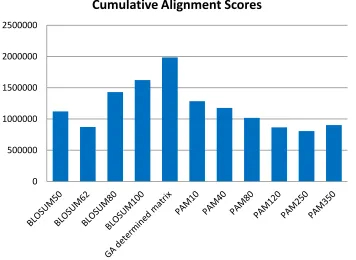
The results of the cumulative alignment scores of the GA determined matrix along with the most
[image:15.612.129.485.146.406.2]commonly used substitution matrices are shown in figure 8.
Figure 8. The cumulative alignment scores of the testing set using the optimal gap-open and gap-extend score of 1 and 0.5 respectively.
The genetic algorithm determined substitution matrix performed the best in the alignment
of the disordered proteins when compared to the other matrices (figure 8). The GA determined
matrix performed two times better than both BLOSUM62 and PAM250. The highest scoring
PAM matrix was PAM10 and the highest scoring BLOSUM was BLOSUM100. It is interesting
to see that the highest scoring PAM and BLOSUM set of matrices are the ones which represent
the least divergent of their respective group. It is also interesting to see that the optimal
gap-open and gap-extend scores are 1 and 0.5 across all the tested matrices. The two most commonly
used matrices for general sequence alignment, BLOSUM62 and PAM250, are one of the lowest
scoring of their respective groups. In contrast, the GA determined substitution scored the highest
resultant in better disordered sequence alignments. This gives evidence that the GA determined
substitution matrix is the best at aligning disordered protein sequences.
0 500000 1000000 1500000 2000000 2500000
Analysis of the genetic algorithm runs
The maximum fitness scores and the average fitness scores of the population were
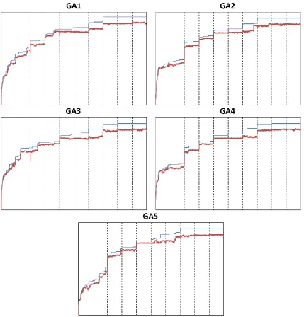
recorded for each generation throughout the genetic algorithm runs. The graph of the runs can
be seen in figure 9. For all five GA runs, the maximum fitness slowly reaches a plateau,
indicating that the genetic algorithm thoroughly searched the solution space before converging to
[image:16.612.93.522.197.645.2]a solution.
In the GA1 run, there is a steady increase in the fitness score through the first 1000
generations (figure 9). At the 1000th generation when the first beam search method was
implemented there is a large increase in the fitness score. This indicates that the GA was aided
by introducing a better solution from a different GA run through the beam search method.
Throughout the GA run, there is a step like increase in the fitness score indicating the beam
search method was working. It is at the third beam search implementation (at the 2000th
generation) that we do not see a increase in the fitness. The lack of increase in the fitness score
is due to the fact that it was this particular GA run that had the best solution, when compared to
the other GA runs, at this particular point in the GA run. The importance of the beam search
method in the GA runs can be seen through generations 2500 to 3000. During this interval, there
is no change in the fitness score. It was only through the beam search method that it was able to
progress out of a stagnant solution and into a different and better solution space. The maximum
fitness score starts to plateau at around the 3500th generation and stays the same even through subsequent beam search methods. This indicates that it has converged to a solution at this point.
The average fitness score is well separated from the maximum score indicating that there is
diversity throughout the genetic algorithm execution and that it was a successful run.
Through the first 1000 generations there is a steady increase in the fitness score also in
the GA2 run, but seems to level off when reaching the 1000th generation. There is a very large increase in the fitness score at the first beam search implementation (generation 1000) indicating
that GA2 was lagging behind compared to the others and was aided by introducing a better
solution from a different GA. The GA2 run took full advantage of the beam search because this
particular run of the GA never gave the optimal solution whenever the beam search was
executed. This is indicated by the step-like increase for every beam search method executed.
The optimal solution was always given to this specific run. Similar to the GA1 run, the
maximum fitness score starts to plateau at around the 3500th generation and stays the same even through subsequent beam search methods. Again, the average fitness score is well separated
from the max score indicating that there is diversity throughout the genetic algorithm execution
and that it was a successful.
Similar to the other GA runs there is a steady increase in the fitness score through to the
generation. Therefore when the first beam search was executed, it was this particular run which
gave the optimal solution to all other GA runs. This was the case also for the second (at
generation 1500) and the fourth (at generation 2500) beam search where the fitness score did not
increase. The maximum fitness score starts to plateau later than the other GA runs, at around the
4000th generation. Again, the average fitness score is well separated from the maximum score indicating that there is diversity throughout the genetic algorithm execution and that it was a
successful run.
The GA4 run is almost identical to the GA2 run. Through the first 1000 generations,
there is a steady increase in the fitness score but seems to level off when reaching the 1000th generation. There is a very large increase in the fitness score at the first beam search
implementation (at generation 1000) indicating that GA4 was lagging behind compared to the
others and was aided by introducing a better solution from a different GA. The GA4 run took
full advantage of the beam search because this particular run of the GA never gave the optimal
solution whenever the beam search was executed, like the GA2 run. Similar to the GA3 run, the
maximum fitness score starts to plateau at around the 4000th generation and stays the same even through a subsequent beam search method. Again, the average fitness score is well separated
from the maximum score indicating that there is diversity throughout the genetic algorithm
execution and that it was a successful.
Again, through the first 1000 generations, there is a steady increase in the fitness score
for the GA5 run. But the rate of increase in the fitness score was lower when compared to all the
other GA runs. Similar to the GA1, GA2, and GA4 runs, there is a very large increase in the
fitness score at the first beam search implementation (generation 1000) indicating that GA5 was
given a more optimal solution by GA3 at this particular point in the run. GA5 gave the optimal
solutions to all the other GA runs, indicated by the lack of an increase in fitness at the fifth beam
search execution (at generation 3000). Like the GA1 and GA2 runs, the maximum fitness score
starts to plateau at around the 3500th generation and stays the same even through subsequent beam search methods. Again, the average fitness score is well separated from the maximum
score indicating that there is diversity throughout the genetic algorithm execution and that it was
a successful.
Throughout every GA run, the fitness scores are characterized by a stepwise increase due
gave the optimal solution for all eight beam search executions. Every GA run benefited from the
others at some point. Another characteristic of the beam search method is the increase in
diversity. As subsequent beam searches were applied, the diversity increased for all runs. By
the time the GA reached the plateau and converged to a solution, there is more diversity in the
population when compared to the beginning of the run. The diversity in the population extends
all the way through to the end which signifies that the convergence to the solution was not due to
the lack of variation of the matrices in the population and that the solution can be trusted.
Determining the best parameter values of the genetic algorithm
In order observe the affect that the pass-through rate, mutation rate and the number of
crossover point values each had on diversity of the population, multiple runs using the same
training set but various parameter values were performed. A brief summary of the results are
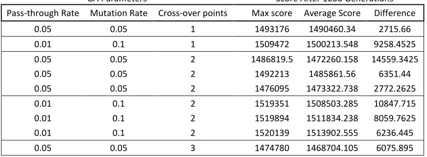
[image:19.612.89.525.409.570.2]shown in table 3.
Table 2. The maximum and average score of GA4 after 1000 generations using various parameter values. The difference is calculated by subtracting the average from the max score. The greater the difference of the average score from the maximum score indicates greater diversity.
GA Parameters Score After 1000 Generations Pass-through Rate Mutation Rate Cross-over points Max score Average Score Difference
0.05 0.05 1 1493176 1490460.34 2715.66 0.01 0.1 1 1509472 1500213.548 9258.4525 0.05 0.05 2 1486819.5 1472260.158 14559.3425 0.05 0.05 2 1492213 1485861.56 6351.44 0.05 0.05 2 1476095 1473322.738 2772.2625 0.01 0.1 2 1519351 1508503.285 10847.715 0.01 0.1 2 1519894 1511834.238 8059.7625 0.01 0.1 2 1520139 1513902.555 6236.445 0.05 0.05 3 1474780 1468704.105 6075.895
Based on the test runs using various GA parameter values, a pass-through rate of 1%, a mutation
rate of 10% and two cross-over points was used for all the final runs of the genetic algorithm.
These values were chosen to be the best because it produced the greatest and more consistent
Discussion
The genetic algorithm determined substitution matrix provided the best alignments of
disordered proteins when compared to both the PAM and BLOSUM set of matrices. It was able
to better align the disordered proteins contained in the testing set indicated by the higher
cumulative score (figure 8). It was identified that the substitution matrices used currently for
general sequence alignments were not acceptable for the alignment of disordered proteins. The
predominant sets of matrices used for sequence alignments used currently are BLOSUM and
PAM. The low scores produced by these matrices give evidence that they align disordered
protein sequences poorly. For example, BLOSUM62 and PAM250 substitution matrices are one
of the most used matrices for sequence alignments, but they are the lowest scoring for disordered
proteins or disordered regions.
There are many parameters when implementing a genetic algorithm which need to be
adjusted to obtain the best solution possible. The genetic algorithm should not converge to a
solution too quickly or the genetic algorithm will not examine the solution space sufficiently. In
order for the genetic algorithm to search the solution space adequately, there must be diversity in
the population. The three parameters which affect the diversity of the population are the
pass-through rate, the mutation rate, and the number of crossover points. In order observe the affect
that each parameter had on diversity, multiple runs using the same training set but various
parameter values were performed. A brief summary of the results are shown in table 2.
Since the scores were taken at one moment in the genetic algorithm run, it would not be
adequate to compare just one run using a specific set of parameters. The rate of convergence can
differ greatly even though the same training set and parameters are used. Therefore multiple
runs using the same parameters were performed to get a general picture of how these value
changes affect diversity (table 2). Although using a pass-through rate of 0.05, a mutation rate of
0.05 and two crossover points yielded the greater difference, there is no consistency in the
difference when the same parameters were executed multiple times. Using a pass-through rate of
0.01, a mutation rate of 0.1 and two crossover points yielded a more consistent diversity. It is
also logically evident that decreasing the pass-through rate, increasing the mutation rate and
increasing the crossover points will cause an increase in the diversity of the population.
values could be performed by observing the difference throughout each passing generation
instead of observing one point in the run. It would be also advantageous to try a wider range of
values. But it is seen through every GA run (figure 9), that diversity in the population was not an
issue and that the used parameter values performed well.
When the final runs of the genetic algorithms reached 1000 generations, it was obvious
that convergence was occurring, but very slowly. This was indicated by the overall similarity of
all five GA solutions. In order to expedite the convergence to the solution without
compromising diversity, the beam search algorithm was implemented for every 500th generation past this point. The beam search allows the optimal solution to be given to all the GA runs. The
GAs which seemed to be lagging behind gets a push forward to an optimal solution. The beam
search does not compromise diversity because each GA population was filled with random
individuals picked from the pool of individuals that did not have the top 10% fitness score.
A suitable substitution matrix for the specific alignment of disordered proteins is needed
and is found. The specific aim of this thesis project has been met and a substitution matrix for
the specific alignment of disordered proteins has been elucidated through the application of
genetic algorithms. Although multiple distinct genetic algorithms were implemented, all of the
GAs converged to one single solution. The convergence of all genetic algorithm runs into one
solution indicates it is the optimal solution for using all training sets. The resulting substitution
matrix out scored all other substitution matrices used currently and gives confidence that the
Reference
1. Wright PE, Dyson HJ. Intrinsically unstructured proteins: re-assessing the protein structure-function paradigm. J Mol Biol. 1999, 293(2), 321-31.
2. Dyson HJ, Wright PE. Intrinsically unstructured proteins and their functions. Nat Rev Mol Cell Biol. 2005, 6(3), 197-208.
3. Dunker AK, Brown CJ, Lawson JD, Iakoucheva LM, Obradović Z. Intrinsic disorder and protein function. Biochemistry 2002, 41(21), 6573-82.
4. Tompa P. Intrinsically unstructured proteins. Trends Biochem Sci. 2002, 27(10), 527-33. 5. Henikoff S, Henikoff JG. Amino acid substitution matrices from protein blocks. Proc Natl
Acad Sci U S A. 1992, 89(22), 10915-9.
6. Dayhoff MO, Schwartz RM, Orcutt BC. “A model of evolutionary change in proteins” in
Atlas of protein sequence and structure, Vol. 5, No. suppl 3. (1978), pp. 345-351.
7. Xie Q, Arnold GE, Romero P, Obradovic Z, Garner E, Dunker AK. The Sequence Attribute Method for Determining Relationships Between Sequence and Protein Disorder. Genome
Inform Ser Workshop Genome Inform. 1998, 9, 193-200.
8. Romero P, Obradovic Z, Li X, Garner EC, Brown CJ, Dunker AK. Sequence complexity of disordered protein. Proteins. 2001, 42(1), 38-48.
9. Williams RM, Obradovi Z, Mathura V, Braun W, Garner EC, Young J, Takayama S, Brown CJ, Dunker AK. The protein non-folding problem: amino acid determinants of intrinsic order and disorder. Pac Symp Biocomput. 2001, 6, 89-100.
10.Brown CJ, Takayama S, Campen AM, Vise P, Marshall TW, Oldfield CJ, Williams CJ, Dunker AK. Evolutionary rate heterogeneity in proteins with long disordered regions. J Mol Evol. 2002, 55(1), 104-10.
11.Dunker AK, Lawson JD, Brown CJ, Williams RM, Romero P, Oh JS, Oldfield CJ, Campen AM, Ratliff CM, Hipps KW, Ausio J, Nissen MS, Reeves R, Kang C, Kissinger CR, Bailey RW, Griswold MD, Chiu W, Garner EC, Obradovic Z. Intrinsically disordered protein. J
Mol Graph Model. 2001, 19(1), 26-59.
12.Sickmeier M, Hamilton JA, LeGall T, Vacic V, Cortese MS, Tantos A, Szabo B, Tompa P, Chen J, Uversky VN, Obradovic Z, Dunker AK. DisProt: the Database of Disordered Proteins. Nucleic Acids Res. 2007, 35(Database issue), D786-93. Epub 2006 Dec 1.
13.Linding R, Jensen LJ, Diella F, Bork P, Gibson TJ, Russell RB. Protein disorder prediction: implications for structural proteomics. Structure. 2003, 11(11), 1453-9.
14.Ward JJ, Sodhi JS, McGuffin LJ, Buxton BF, Jones DT. Prediction and functional analysis of native disorder in proteins from the three kingdoms of life. J Mol Biol. 2004, 337(3), 635-45.
15.Dosztányi Z, Csizmok V, Tompa P, Simon I. IUPred: web server for the prediction of intrinsically unstructured regions of proteins based on estimated energy content.
Bioinformatics. 2005, 21(16), 3433-4. Epub 2005 Jun 14.
16.Anita Thengade and Rucha Dondal. Genetic Algorithm - Survey Paper. International
Journal of Computer Applications. 2012, Issue 5, pp. 25 – 29.