New computational methods and plant models for evolutionary genomics

(1)

New computational methods and plant

models for evolutionary genomics

Kevin D. Murray

A thesis submitted for the degree of

Doctor of Philosophy of

The Australian National University

(2)

(3)

This thesis was typeset in URW Garamond using the LA_{TEX typesetting system originally} developed by Leslie Lamport, based on TEX created by Donald Knuth, and using pandoc,

(4)

I declare that the research presented in this Thesis represents original work that I carried out during my candidature at the Australian National University, except for collaborator’s contributions to multi-author papers incorporated in the Thesis, which are detailed in each chapter’s prefix.

(5)

From forest caves, and azure skies We crashed upon this earth The years, they passed And so did we

But resistance would be bought

(6)

Acknowledgements

This thesis would never have been possible without the support of an enormous number of people, too many to name individually. Nonetheless, you all have my gratitude.

Firstly, I must thank all those who have advised and mentored me over the last four years. Justin, thank you for everything, I would be neither as competent nor confident as a scientist without the advice, encouragement, and opportunities you’ve given me during and before my PhD. To Norman, who co-supervised my work on what became kWIP, thanks for the belief you had in my daft ideas, and for your enthusiasm and continuing friendship. To Rose, who co-supervised my recent work onEucalyptus, thanks for your endless and cheerful help, and for your hospitality during my frequent visits to Armidale. To Sylvain, my late co-supervisor, your friendly advice influenced much of the work I present here, and you have been greatly missed. To my panel, Barry, Gavin, and Eric, thank you for all the encouragement and advice you’ve given. And an extra thanks to Barry for the opportunities you gave me as an undergraduate, without which I doubt I would have commenced a PhD.

I must also thank my co-authors and collaborators on the work I present here: Chrisfried, Cheng Soon, Jared, Pip, Steve, Riyan, Niccy, Jasmine, Helen, and anyone I’ve forgotten. Thanks also to the great communities in which I’ve worked, particularly the members of the Borevitz, Pogson, and Andrew labs, and my EEG and Plant Science PhD student cohort. Thanks to Tim Brown and the whole APPF team, who’ve been rewarding colleagues with whom to plumb the murky depths of phenomics data. Thanks to the international labs who I have visited and/or collaborated with: Titus Brown and lab (particularly Camille Scott, Luíz Irber, and Michael Crusoe), for your help withkhmerand hospitality in Davis; Detlef Weigel and lab for hospitality in Tübingen; and Loren Rieseberg and lab for hospitality in Vancouver. Thanks to the developers of several tools, whose helpful advice enabled their use: Gideon Bradburd, Timothy Bilton, Johannes Köster, Titus Brown’s lab, Vince Buﬀalo, Reed Cartwright, Paul Staab, and Jonas Meisner.

On a personal note, thank you to all my dear friends, whose friendship has somehow kept me approximately sane through the trials of a PhD. Thank you to my family, for getting me to the point that I could start a PhD, and for getting me through it. Most of all, thank you to Luisa, my dearest companion. You are incredible, and have made the last 5 years the best of my life.

(7)

Thesis Abstract

This thesis is in the service of a greater understanding of the genetic basis of adaptive traits. Chapter 1 introduces background literature relevant to this thesis. Chapters 2, 3, and 4 de-velop novel methods and software for the analysis of genetic sequencing data. Chapter 5 details a large collaborative project to establish genetic resources in the model cereal Brachy-podium, and perform a genome-wide association study for several agriculturally-relevant traits under two climate change scenarios. Chapter 6 investigates the spatial genetic patterns in two species of woodland eucalypt, and determines the landscape process that could be driv-ing these patterns. Finally, Chapter 7 summarises these works, and proposes some areas of further study.

In Chapters 2 and 3, I develop methods that enable the analysis of Genotyping-by-sequencing data. Axe, a short read sequence demultiplexer, demultiplexes samples from multiplexed GBS sequencing datasets. I show Axe has high accuracy, and outperforms previously published software. Axe also tolerates complex indexing schemes such as the variable-length combinatorial indexes used in GBS data. Trimit and libqcpp (Chapter 3) implement several low-level sequence read quality assessment and control methods as a C++ library, and as a command line tool. Both these works have been published in peer-reviewed journals, and are used by numerous groups internationally.

In Chapter 4, I develop kWIP, a de novo estimator of genetic distance. kWIP enables rapid estimation of genetic distances directly from sequence reads. We first show kWIP out-performs a competing method at low coverage using simulations that mimic a population resequencing experiment. We propose and demonstrate several use cases for kWIP, including population resequencing, initial assessment of sample identity, and estimating metagenomic similarity. kWIP was published in PLoS Computational Biology.

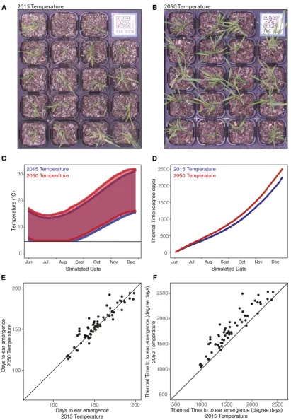
In Chapter 5, I present the results of a large, collaborative project that surveys the global genetic diversity of the model cerealBrachypodium. We amass a collection of over 2000 acces-sions from the Brachypodium species complex. Using GBS and whole genome sequencing we identify around 800 accessions of the diploidBrachypodium distachyon, within which we

(8)

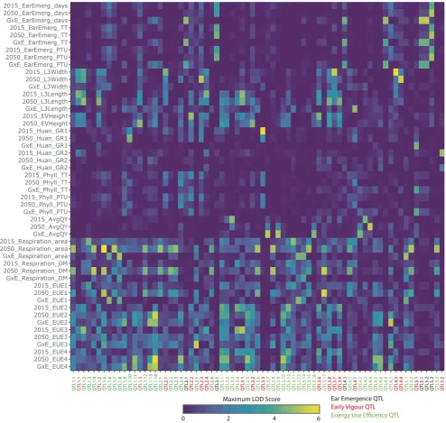
find extensive population structure and clonal families. Through population restructuring we create a core collection of 74 accessions containing the majority of the genetic diversity in the “A genome” sub-population. Using this core collection, we assay several phenotypes of agricultural interest including early vigour, harvest index and energy use eﬃciency under two climates, and dissect the genetic basis of these traits using a genome-wide association study (GWAS). This work has been published in Genetics; I am co-first author with Pip Wilson and Jared Streich, having lead many genomic analyses.

In Chapter 6, I perform a study of landscape genomic variation in two woodland eucalypt species. Using whole genome sequencing of around 200 individuals from around 20 localities of bothE. albensandE. sideroxylon, I find incredible genetic diversity and low genome-wide inter-species diﬀerentiation. I find no support for strong discrete population structure, but strong support for isolation by (geographic) distance (IBD). Using generalised dissimilarity modelling, I further examine the pattern of IBD, and establish additional isolation by envi-ronment (IBE).E. albensshows moderately strong IBD, explaining 26% of the deviance in the genetic distance using geographic distance, and an additional 6% of the deviance is explained by incorporating environmental predictors (IBE).E. sideroxylonshows much stronger IBD, with 78% of the deviance explained by geography, and stronger IBE (12% additional deviance explained). This work will soon be submitted for publication.

(9)

2 Axe: rapid, competitive sequence read demultiplexing using a trie 32 3 libqcpp: A C++14 sequence quality control library 35 4 kWIP: The k-mer weighted inner product, a de novo estimator of genetic simi-larity 37 5 Global Diversity of the Brachypodium Species Complex as a Resource for Genome-Wide Association Studies Demonstrated for Agronomic Traits in Response to Climate 55 6 Landscape drivers of genomic diversity and divergence in woodland eucalypts 71 6.1 Abstract . . . 72

6.2 Introduction . . . 72

6.3 Methods . . . 75

6.4 Results . . . 82

6.5 Discussion . . . 92

(10)

6.7 Supplementary information . . . 106

7 Thesis Discussion 119 7.1 Thesis progress . . . 119

7.2 New computational methods . . . 119

7.3 Brachypodium as a model cereal . . . 122

7.4 Landscape drivers of eucalypt genetic diversity . . . 123

7.5 Evolutionary genomics in the Anthropocene . . . 127

A Other published works 136

(11)

Chapter 1 Thesis Introduction

This thesis concerns the genomics of adaptation to environment in plants. The works that comprise this thesis address a wide range of questions in several systems, and establish novel methods to do so. They range from the development of improved algorithms for vital early stages of modern sequencing analysis pipelines, to a study of the landscape drivers of spatial genetic patterns inEucalyptus. They span multiple generations of improvement in genome sequencing technology, highlighting the incredible pace of technological improvement this field is experiencing. This thesis also demonstrates that the leading edge of genomics can only be reached through the development of novel statistical and computational tools, and their collaborative application to large datasets.

1.1 Adaptation genomics: the genomic biology of

popula-tions, landscapes, and quantitative traits

The phenotype of an individual is the expression of its genome in the environment it experi-ences. Adaptation genomics centers on the triad of genotype, phenotype, and environment, and interrogates the processes linking these concepts (Bragg et al., 2015; Radwan Jacek and Babik Wiesaw, 2012; Stapley et al., 2010). Adaptation genomics asks a series of questions re-lated through this triad: What potentially adaptive genetic diversity exists? What phenotypic diversity is expressed? How is this diversity distributed and filtered across the landscape? Which loci underpin variation in traits? Is there evidence for selection at these loci?

The fields of population, landscape, and quantitative genomics form the backbone of this thesis. These fields study intra- and interspecific variation from a variety of angles, and produce findings that can assist management of ecosystems, both natural and agricultural.

(12)

For example, an understanding of the environmental drivers of genetic variation over the landscape can help restore and manage natural ecosystems (Broadhurst et al., 2008; Hoﬀmann et al., 2015). In an agricultural context, dissecting the genetic basis of phenotypic traits enables precise selection of advantageous genotypes to improve both yield and resilience (Ainsworth and Ort, 2010; Fernie et al., 2006). The study of genetic diversity is essential to all these questions.

1.1.1 Genetic diversity

A genetic polymorphism is defined here as a locus at which mutation has given rise to at least two distinct allelic states that occur in multiple individuals. Over time the frequencies of these states may change (i.e., evolution), through either random drift or selection. Multi locus genetic diversity is a quantification of these polymorphisms among individuals within and between populations. It is the substrate of evolution controlling heritable phenotypic variation that is subject to natural selection underlying adaptation.

In most organisms, a proportion of genetic variation is spatially autocorrelated–that is, genetic variation is not randomly distributed over the geographic range of a species (Sokal and Oden, 1978a, 1978b). Genetic spatial autocorrelation arises through a variety of pro-cesses, both neutral and adaptive (Diniz-Filho et al., 2009). Many of the processes governing spatial autocorrelation of allele frequencies are not the result of any adaptive separation, for example outbreeding over limited distances or expansion from an ancestral refugia (Sokal and Oden, 1978b). Strong selection on specific traits may lead to reduced gene flow between diﬀering environments (isolation by environment), perhaps because of unfit migrants (Wang and Bradburd, 2014).

1.1.2 Genetic isolation and diﬀerentiation

Genetic diﬀerentiation is due to neutral processes including drift, particularly in small pop-ulations, non-random mating, and non-random migration. Isolated subpopulations with re-duced gene flow relative to drift will fix mutations that diﬀerentiate them (Hahn, 2018). Discrete population structure is the result of low gene flow between two (or more) subpop-ulations, relative to gene flow within each subpopulation. There are innumerable potential causes of reduction in gene flow, some geographic (e.g., separation by large swathes of in-tolerable habitat), and others non-geographic (e.g., divergence in flowering time leading to temporal isolation).

(13)

In contrast to discrete population structure, Isolation by Distance (IBD; Wright, 1943) is the observation that proximate individuals have higher relatedness than distant individuals; IBD is a ubiquitous pattern (Meirmans, 2012). IBD may vary in strength over the landscape and across the genome. In particular, the relationship between genetic and geographic dis-tance need not be linear. While there are many specific causes of IBD, fundamentally it is the result of the probability of gene flow between two individuals being some function of their geographic separation (i.e., non-random mating). Technically, the pattern of IBD is the integral through time of this non-random mating, and the extent of non-random mating may vary through time. Additionally, certain demographic histories can result in a pattern of IBD, for example postglacial expansion from a refugia (Holliday et al., 2010; Meirmans, 2012).

Isolation by Environment (IBE; Wang and Bradburd, 2014) extends the concept of Iso-lation by Distance to environmental causes of non-random mating over the landscape. IBE occurs when individuals in dissimilar environments exchange less genetic material than indi-viduals in similar environments, controlling for reduced gene flow caused by geographic sep-aration. IBE can have many causes, including selection, reduced fitness of inter-environment migrants or hybrids, and biased dispersal. Importantly, although local adaptation at particu-lar loci can ultimately lead to genome wide IBE, evidence of IBE is not evidence of selection: a variety of neutral processes can generate similar patterns (e.g., postglacial recolonisation a la IBD; Wang and Bradburd, 2014; Holliday et al., 2010). Typically, environmental dis-tance is calculated from interpolated predictions (e.g. of climate; Xu and Hutchinson, 2013; Fick and Hijmans, 2017). Estimation of IBE assumes the underlying modelled environmental variables are accurate throughout the life of the individual—a tenuous assumption for cer-tain variables in the case of long-lived organisms. Discriminating between patterns that are purely neutral, neutral but are side eﬀects of selection (i.e. linked selection), and patterns that are a direct result of selection is challenging, and typically requires orthogonal information (Holliday et al., 2010; Meirmans, 2012; Wang and Bradburd, 2014). For instance, evidence of reduced fitness of inter-environmental immigrants can confirm local adaptation (Wang and Bradburd, 2014; e.g. in Keller et al., 2011), but do not get at the underlying genetic ba-sis. Such experiments (e.g. provenance trials) are expensive and time consuming, especially in trees. Therefore, I make no attempt to do so in this thesis, testing only for patterns of correlation between geographic/environmental distance and genetic distance.

(14)

1.1.3 Conservation: migration of ecotypes vs increasing adaptive

poten-tial

The global climate is changing, and entire ecosystems are being lost through a variety of human activities (e.g. deforestation). One application of finding genetic isolation by envi-ronment and geography is to assist conservation and revegetation eﬀorts at a given locality (Broadhurst et al., 2008; Supple et al., 2018). However, looking forward, local adaptation to (past) environment does not necessarily indicate suitability to the future environment at a given locality (Wogan and Wang, 2018). Even when models of IBD and IBE are used to predict genomic suitability from predicted future climate data, humility regarding model projections should guide recommendations. This is especially true given predictions suggest that not only will environmental means shift with climate change, but variances will increase (Thornton et al., 2014). This suggests that a broad understanding of the landscape processes governing spatial patterns of genetic variation is more urgent than discovering locally-adapted loci in each habitat, especially given limited resources (Kardos and Shafer, 2018). In any case, a focus on preserving adaptive potential is key to any restoration and conservation works, rather than attempts to discover “perfectly adapted germplasm” for revegetation (Broadhurst et al., 2008; Hoﬀmann et al., 2015; Weeks et al., 2011).

1.2 Discovering genetic variation

Virtually all modern studies of genetics now use either short or long read high throughput sequencing (Mardis, 2008; Metzker, 2010). Such methods generate truly staggering quantities of data within which genetic variation must be discovered (Pfeifer, 2017). Many molecular and computational methods exist to discover genetic variation, of which I will discuss those pertinent to the work I present in this thesis. Additionally, I will discuss the fact that oﬀ-the-shelf molecular and computational tools are often not suited to non-human experiments, mandating the development of new tools as part of a particular biological project.

Given sequencing machines do not provide full diploid genome sequences directly, genetic variation is typically discovered as variation among samples relative to a reference genome (Li, 2011; Pfeifer et al., 2014). This process, termed variant calling, statistically integrates all data across samples to determine if each position in the reference genome is variable, and subse-quently to determine the most likely genotype at each locus for each individual. A variety of computational and statistical approaches have been developed to perform this task, for example mpileup (Li, 2011), freebayes (Garrison and Marth, 2012) and GATK’s

(15)

Caller (DePristo et al., 2011; McKenna et al., 2010). These algorithms were largely designed to work with relatively high coverage (e.g. 15 fold), and with a reference genome that is not very diverged from samples of interest. Where these assumptions are not met, various errors and/or biases may be introduced, both in genotype calls and subsequent inferences based upon them (Brandt et al., 2015; Han et al., 2014; Nielsen et al., 2011). To combat these issues, various methods that aim to preserve uncertainty inherent in less than saturating se-quencing coverage. This uncertainty can be incorporated into typical population genetic inference, e.g. ANGSD (Fumagalli et al., 2013; Korneliussen et al., 2014, 2013). These meth-ods estimate the most likely values of the statistic of interest (e.g. calculation of population genetic statistics, or inter-sample distances) given the sequence data, rather than given the called genotypes. This diﬀerence allows these methods to improve the accuracy and reduce the bias of their estimates, particularly on low-coverage data (Fumagalli, 2013; Korneliussen et al., 2014, 2013).

Necessarily, discovering genetic variation involves integrating across many samples. How-ever, even with methods designed to operate on low coverage data, reliably assaying a sample’s genotype requires a significant sequencing cost. Given limited budgets, this presents a trade-oﬀ: more samples, with less data per sample, or fewer samples with more data? In nearly all cases, more samples with a modest amount of data represents the best statistical power for some fixed investment (Fumagalli, 2013; Kliebenstein, 2012; Li et al., 2011; Pasaniuc et al., 2012).

1.2.1 Dimensions of Genomic Complexity

Genomic complexity was considered within a reference haploid genome, measured perhaps by genome size, repeat content or ploidy. With population re-sequencing, there is another axis to consider, that of genetic diversity across samples. In this dimension, genetic diversity could be considered to be the total or average pairwise diversity among samples in a pop-ulation. The units of this diversity axis would be metrics such as π, population structure and F_ST, or the extent of linkage disequilibrium (LD; Hahn, 2018). In studies that aim to determine functional genetic variation, both dimensions of genome complexity need to be considered as they determine the experimental design and cost. As both samples and poly-morphisms show statistical dependence (i.e. structure and LD), missing data can be imputed across related individuals and along the genome (Browning and Browning, 2007; Howie et al., 2009; Marchini and Howie, 2010). This can sometimes dramatically reduce costs but can also limit resolution and power (fig. 1.1).

(16)

Arabidopsis

Pine

Wheat

Genome Complexity

Genetic Div

ersity

Figure 1.1: Dimensions of genomic complexity. In many genomic studies (partic-ularly genome assembly), genome complexity describes the size and complexity of a single haploid genome. In studies of evolutionary genetics, we must also consider an orthogonal axis: genetic variability. The size and complexity of a single haploid genome determines the cost of reliably assaying the whole genome sequence of one individual, however imputation can leverage statistical dependence between loci to re-duce the eﬀective cost of sequencing a population. Thus, the total cost of genotyping a population in a resequencing study is some combination of both genomic complexity and genetic variation (specifically LD).

(17)

Regardless of the specific amount of structure and LD in the sampled genomes, a reference genome is either required or extremely useful (Pfeifer, 2017; although see e.g. Audano et al., 2018). In particular, polymorphism-wise analyses like GWAS require a reference genome to order markers, and to anchor them to genes. Ordered markers are also crucial for inference of some population metrics, particularly those whose currency is haplotypes (e.g. selective sweep detection; Hahn, 2018; Pavlidis et al., 2013; discovery of introgressed segments; Bragg et al., 2015). Thankfully, modern long-read sequencing methods and long read-specific as-semblers make assembly of at least draft genomes achievable on limited budgets of time and money (e.g. Michael et al., 2018). I have also developed non-reference approaches to look at sample relatedness (Chapter 4; Murray et al., 2017) which can then prioritize selection of distantly related samples for reference genome assembly.

1.2.2 Specifics of sequencing methods

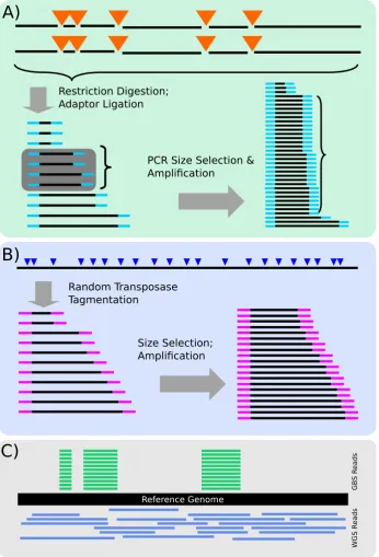
Until relatively recently, it remained too expensive for most researchers to sequence whole genomes with sufficient sample size for quantitative study of genetic variation. Reduced rep-resentation sequencing methods aimed to reduce sequencing costs by assaying only a fraction of the genome. A large range of such methods exists, employing various molecular methods to subset the genome (Baird et al., 2008; Blumenstiel et al., 2010; Elshire et al., 2011; Faircloth et al., 2015; Morris et al., 2011; Peterson et al., 2012; Smith et al., 2014). One such method employed in this thesis is Genotyping by Sequencing (GBS; Elshire et al., 2011). GBS uses restriction enzymes to fragment each sample’s genome, and sequencing libraries are created only for genome regions near these restriction sites. Then, many hundreds of samples may be multiplexed and sequenced on one sequencing run, drastically reducing the sequencing cost per sample (Elshire et al., 2011). While such data is of acceptable quality and quantity for most genome-average analyses (e.g. genetic distance, detecting population structure), it often assays an insufficient fraction of the genome to be used in many genome-wide polymorphism-wise analyses (unless LD is very extensive). Additionally, GBS data is often plagued with a large proportion of missing data, a lack of reproducibility, strong batch effects, and strong allelic bias (Bilton et al., 2018; Lowry et al., 2017).

In contrast to GBS, whole-genome shotgun sequencing provides data on (nearly) all DNA present in each sample. In such methods, sequencing libraries are created from short frag-ments of DNA from approximately random genome positions (including organellar and other genomes present in a sample; Bentley et al., 2008). As a consequence, these meth-ods require significantly more sequencing per sample than reduced representation data, but

(18)

generally produce datasets of higher quality, and assay (nearly) all polymorphisms present in some population (Fuentes-Pardo and Ruzzante, 2017; Lowry et al., 2017). With the ad-vent of cheaper sequencing and development of cost-eﬃcient library preparation ( Jones et al., 2018), WGS became economic at increasing scales, to the point where WGS costs are now approximately equal the cost of GBS at the beginning of my PhD.

1.2.3 Computational method development

The development of robust and efficient computational methods often lags behind the devel-opment of ever more efficient molecular methods. Therefore, to use cutting edge molecular methods, one must often develop computational tools specific to some dataset or protocol. This is especially true in adaptation genomics, where the experimental designs (such as those discussed below) diverge significantly from those that many “off-the-shelf” analysis methods expect. The methods required range from smaller utilities to efficiently solve problems with known solutions, to large programs implementing entirely new metrics or algorithms.

While there are only a few high-level steps in any analysis (e.g. alignment to reference, variant calling), each high-level task is often performed by several smaller tools. In many cases, these tools are application- or datatype-specific. The use of custom, cost-conscious molecular protocols in the chapters of this thesis required the development of certain tools. One example is the requirement for improved demultiplexing software for GBS data. In-creasing sequencing capacity lead to inIn-creasing amounts of sample pooling, in the case of GBS using combinatorial, paired end, indexing. However, at the time, no methods were able to de-multiplex this data accurately and eﬃciently. This required the development of tools to perform this crucial early stage of GBS data analysis (Chapters 2 and 3).

As outlined above, discovering genetic variation is computationally intensive, and typ-ically requires a reference genome. However, at least in the early stages of analysis, one is simply interested in the genetic similarity of samples. Therefore, eﬃcient methods to rapidly estimate of genetic similarity directly from sequencing data are required. Such methods have the potential to estimate genetic distances without reference genome bias, and to verify that individuals belong to the correct genetic lineage before conclusions are drawn using misla-belled, or misidentified samples. Importantly, such methods would be sequencing-method agnostic, unlike reference-free methods designed to work only with reduced representation methods.

Alignment-free sequence comparison algorithms satisfy many of these requirements. Alignment-free methods generally operate by decomposing sequences (or sequence data)

(19)

Restriction Digestion; Adaptor Ligation

PCR Size Selection & Ampliﬁcation

A)

Random Transposase Tagmentation

Size Selection; Ampliﬁcation

B)

GB

S R

eads

WGS R

eads

Reference Genome

[image:19.595.126.473.103.613.2]

C)

Figure 1.2: Overview of GBS and WGS sequencing methods and data.A) GBS

se-quencing protocol: briefly, genomic DNA is digested with restriction enzymes, adap-tors are ligated, and PCR used to size-select and amplify libraries. B) WGS sequencing protocol: briefly, adaptors are directly transposed into genomic DNA at random posi-tions, amplified with PCR, and size-selected using electrophoresis. C) GBS and WGS data aligned to a reference genome. GBS data aligns to quantised positions, and has higher coverage at covered positions. WGS data aligns approximately uniformly across the genome, and has lower coverage for a given sequencing volume.

(20)

into kmers, i.e. substrings of length k (e.g. Song et al., 2014; Forêt et al., 2009; Sims et al., 2009; Tang et al., 2014). Recently, several algorithms enabling de novo sequence compar-ison have been published, generally attempting to reconstruct phylogenetic relationships from sequencing reads. Spaced (Leimeister et al., 2014; Morgenstern et al., 2015) uses

the Jensen-Shannon distance on spaced kmers for accurate phylogenetic reconstruction.

Cnidaria(Aflitos et al., 2015) andAAF(Fan et al., 2015) use the Jaccard distance to estimate

phylogenetic distances.Mash(Ondov et al., 2016) uses a MinHash approximation of Jaccard

distance to the same effect but with extreme computational efficiency. My contribution, kWIP (Chapter 4) uses a weighted inner product to determine distance and is well suited for within species differentiation.

1.3 Experimental designs to uncover drivers of spatial

ge-netic diversity

Landscape genomic studies typically form two phases, an exploratory descriptive phase fol-lowed by one or more targeted, hypothesis-driven experiments guided by patterns uncov-ered in the first phase (Bragg et al., 2015). In each phase, many samples are obtained, across the relevant geographic and environmental range (i.e. initially the whole range of the study species, then across specific environmental gradients relating to hypotheses under consider-ation; Bragg et al., 2015; Wang and Bradburd, 2014). One then employs population-wide sequencing to find genetic variation, either using reduced-representation or whole-genome methods.

Once genetic variation has been ascertained, the descriptive phase seeks to establish genome-wide background patterns of gene flow and isolation across the landscape. There are many approaches to this task. Several methods model genetic distance (or similarity, e.g. allelic covariance) as a function of geographic and/or environmental distances. Tradi-tionally, methods like mantel and partial mantel tests, and multiple regression on matrices were employed (Legendre and Legendre, 2012; Lichstein, 2007; Mantel, 1967; Smouse et al., 1986), however in some scenarios these have undesirable statistical properties, including a high false positive rate (Guillot and Rousset, 2013). More modern methods address some of these concerns, including generalised dissimilarity modelling (GDM; Ferrier et al., 2002, 2007), and BEDASSLE (Bradburd et al., 2013). All these methods establish the extent to which genetic distances (and therefore underlying allele frequencies) are spatially and environmentally autocorrelated as a result of non-random gene flow. Importantly,

(21)

these models of genome-wide average distance are overwhelmingly influenced by neutral segregating mutations, and are not in themselves evidence of any adaptive process, though selection may influence gene flow, and generate this pattern (Wang and Bradburd, 2014).

The subsequent hypothesis driven analyses could take many forms. One may wish to find individual loci associated with specific environmental characters, amounting to correlation of allele frequency with some environmental gradient. Therefore, specific tests are required, for example BayEnv (Günther and Coop, 2013) or latent-factor mixed models (Stucki et al., 2017). Such polymorphism-wise analyses are best performed using whole-genome sequencing data, to ensure all genetic variation is tested.

Complementary experiments examine environmentally adaptive trait variation, likely fil-tered by the environment, to dissect the genetic basis of these traits using GWAS. This would involve growth of individuals from across some environmental gradient in common condi-tions, and phenotyping of traits relevant to environmental gradients of interest (e.g. water use eﬃciency along an aridity gradient). Diﬀerences in fitness could also be directly tested, perhaps using reciprocal transplants along some environmental gradient to test for local adap-tation. In all these experiments, one must correct not only for any population structure (a laGWAS), but also for the genome-wide background isolation by distance and environment that would cause neutral loci to correlate with environmental gradients or trait variation. For this reason, the power of such analyses is inversely proportional to the strength of genome-wide IBE and IBD and population structure. Chapter 6 presents a descriptive analysis of the patterns of IBD and IBE, and does not perform any of these more targeted, hypothesis-driven experiments.

1.4 Experimental designs for uncovering genetic basis of

quantitative traits

Traits are heritable characters of an individual, and quantitative traits are the subset of traits whose values form an approximately normal distribution when quantified in some popula-tion (Lynch and Walsh, 1998). Uncovering the genetic basis of such traits involves statistical association of trait values with genetic variation across the genome. The strength of this statistical association is assessed at each polymorphic locus. Loci where genetic variation and trait variation appear correlated are considered a quantitative trait locus (QTL). This association is purely statistical without further investigation of QTL, perhaps in the form of functional study of genes contained within the QTL of interest. In particular, in most studies

(22)

the polymorphisms underlying QTL are predominantly not causal, rather their allelic state is correlated with that of causal mutations (linkage disequilibrium; LD), and causal mutations themselves may not even be assayed. These studies can be conducted in natural populations (i.e. genome-wide association studies; GWAS) or within artificially-created mapping popula-tions, e.g. recombinant inbred lines or nested association mapping populations (often termed QTL mapping).

In species with low outbreeding rates, finding sufficient genetic variation is the hard part of GWAS. To do so, one typically sequences many thousand individuals, and reduces this to a core set that maximises genetic diversity while minimising population structure and other confounding factors; an approach termed “population restructuring” (Brachi et al., 2011). At least for this initial restructuring, whole-genome data is not required and studies typically use a cost-effective reduced representation sequencing approach (Brachi et al., 2011; Elshire et al., 2011). However, merely choosing a subset of samples is not always sufficient to create a powerful population. One can obtain more diverse and less structured populations either through targeted re-sampling of diverse regions, or the creation of artificial mapping populations that release genetic diversity from background structure (Brachi et al., 2011). Once a diverse population has been obtained, it can then be sequenced using whole genome sequencing, providing polymorphism data required for a GWAS.

In contrast, finding diversity in outbred species is less challenging than accurately assaying it. Outbred species tend to have high genetic diversity, with very large numbers of polymor-phisms, and often relatively less correlation between these polymorphisms (i.e. low LD; Ny-bom and Bartish, 2000). In such cases, population restructuring is less likely to be required, and whole-genome sequencing may be used immediately (Brachi et al., 2011). However, very large sample sizes are often required to achieve a statistically powerful polymorphism-wise association study, especially when the number of polymorphisms is very large (Pfeiﬀer and Gail, 2003; Purcell et al., 2003).

Regardless of the genetic diversity and the population genetics of the sample set at hand, plants must be grown and traits of interest must be phenotyped, typically using automated high-throughput phenotyping (Brown et al., 2014). Plants may be grown in laboratory ditions, with the downside that their growth conditions are unrealistic, with obvious con-sequences on the expression of traits. To combat this, one may grow plants in lab growth conditions that attempt to mimic the basic environmental characters of some region (e.g. light intensity and spectral quality, temperature, day length). Genotype-environment interactions may be investigated, with plants grown under multiple environments, and genetic basis of

(23)

some trait determined independently in each condition.

1.5 Biological case studies

1.5.1 Brachypodum

The genusBrachypodiumis collectively an established model system of grass (and in partic-ular cereal) biology, and is phylogenetically situated among the world’s major cereal crops (Draper et al., 2001; reviewed in Kellogg, 2015). B. distachyonhas received particular atten-tion, with its small, diploid genome, rapid life cycle, and small stature making it a tractable organism for laboratory study. The development of a model cereal is of particular interest given the often very large, complex genomes, long life cycles, large stature of crop species, and the large divergence, in phenotypic and phylogenetic terms, between these crops and the established model dicot Arabidopsis thaliana(Brkljacic et al., 2011). Significant variation in ploidy and genome architecture exists inBrachypodium, for example the commonB. hybridum is an allo-tetraploid (2n=4x) betweenB. distachyonandB. staceii(Catalán et al., 2012). Such ploidy variation enhances the utility of this species complex as a model of cereal evolution, as many cereals have similar variation in ploidy and genome architecture. Studies of genetic diversity inB. distachyonfound moderate genetic variation, confounded by strong structure and inbreeding, and extensive migration with little recombination (Filiz et al., 2009; Vogel et al., 2009; reviewed in Scholthof et al., 2018).

Eﬀorts to establishBrachypodiumas a model for cereal quantitative genetics are ongoing, with a B. distachyon reference genome assembly first released in 2010 (Bd21; The Interna-tional Brachypodium Initiative, 2010), and an independent assembly of Bd21-3 available pre-publication from JGI Phytozome release 11. The first sizeable collection of wild accessions and associated phenotypes was released in 2014 (Tyler et al., 2014). Short satellite repeat (SSR) markers and a collection of inbred lines were developed from samples of Turkish origin (a diversity hotspot; Vogel et al., 2009). Collections of hundreds of accessions were developed, primarily as part of the USDA’s Germplasm Resources Information Network (Scholthof et al., 2018). However, at the outset of the collaborative project I present in Chapter 5, no global collections of a suitable size for GWAS were publicly available.

(24)

1.5.2 Eucalyptus

The genus Eucalyptus comprises more than 800 described taxa, with natural distributions restricted to Australia and surrounding tropical islands. Eucalypts are the dominant and key-stone tree species in most Australian habitats, and some species are hardwood forestry species of global significance. Eucalypts range in form from large shrubs to the world’s tallest an-giosperm (“Centurion”, aE. regnansin Tasmania that recently reached 100 metres; National Register of Big Trees, 2013). Thornhill et al. (2015) estimate the age of the genusEucalyptus to be approximately 70 My. The genus is classified into three main subgenera which each contain a hierarchical grouping of species into series and series to sections (Pryor and John-son, 1971). For example, Chapter 6 concerns two species,E. albensandE. sideroxylon, from two different series (buxaelesandmelliodoriae) within the section Adnataria of the subgenus Symphiomyrtus. Many species withinEucalyptusreadily hybridise, often forming fertile off-spring and hybrid swarms (e.g. Pryor, 1953). Eucalypts are generally pollinated by generalist insect or vertebrate pollinators, and preferentially outcross (Potts and Gore, 1995). Broadly, previous genomic studies of widespread eucalypt species reveal very high genetic diversity, and low population structure and isolation by distance and/or environment (e.g. Potts and Jordan, 1994; Bloomfield et al., 2011; Gauli et al., 2014; Griffin et al., 1987; Supple et al., 2018).

1.6 Chapter summaries

This thesis presents work that views evolutionary genetics from a wide variety of angles. Chapters 2 and 3 describe the development of new computational methods to analyse GBS data. Chapter 4 describes kWIP, an estimator of genetic distance that operates directly on short read sequencing data. Chapter 5 describes a large eﬀort to establish genetic resources for GWAS in the model cereal Brachypodium, and uses these resources for a GWAS on agronomic traits under simulated climate change. Chapter 6 presents recent work that seeks to identify the landscape drivers of genetic divergence and diversity in two woodland eucalypt species. Chapter 7 summarises these works, and proposes several avenues for further investigation. Chapters 2, 3, 4, and 5 outline works that have been accepted in peer reviewed journals, and accepted articles are replicated in this thesis for convenience.

(25)

1.7 References

Aflitos SA, Severing E, Sanchez-Perez G, Peters S, de Jong H, de Ridder D.2015. “Cnidaria: Fast, reference-free clustering of raw and assembled genome and transcriptome NGS data.” BMC Bioinformatics16:352. doi:10.1186/s12859-015-0806-7

Ainsworth EA, Ort DR.2010. “How Do We Improve Crop Production in a Warming

World?” Plant Physiology154:526. doi:10.1104/pp.110.161349

Audano PA, Ravishankar S, Vannberg FO, Berger B.2018. “Mapping-free variant call-ing uscall-ing haplotype reconstruction from k-mer frequencies.” Bioinformatics34:1659–1665. doi:10.1093/bioinformatics/btx753

Baird NA, Etter PD, Atwood TS, Currey MC, Shiver AL, Lewis ZA, Selker EU, Cresko

WA, Johnson EA. 2008. “Rapid SNP Discovery and Genetic Mapping Using Sequenced

RAD Markers.”PLoS ONE 3:e3376. doi:10.1371/journal.pone.0003376

Bentley DR et al. 2008. “Accurate whole human genome sequencing using reversible terminator chemistry.” Nature456:53–59. doi:10.1038/nature07517

Bilton TP, Schofield MR, Black MA, Chagné D, Wilcox PL, Dodds KG. 2018.

“Accounting for Errors in Low Coverage High-Throughput Sequencing Data When Con-structing Genetic Maps Using Biparental Outcrossed Populations.” Genetics 209:65–76. doi:10.1534/genetics.117.300627

Bloomfield JA, Nevill P, Potts BM, Vaillancourt RE, Steane DA.2011. “Molecular genetic variation in a widespread forest tree species Eucalyptus obliqua (Myrtaceae) on the island of Tasmania.” Aust J Bot59:226–237. doi:10.1071/BT10315

Blumenstiel B et al. 2010. “Targeted Exon Sequencing by In-Solution Hybrid Selection.” Current Protocols in Human Genetics66:18.4.1–18.4.24. doi:10.1002/0471142905.hg1804s66

Brachi B, Morris GP, Borevitz JO. 2011. “Genome-wide association studies in plants: The missing heritability is in the field.” Genome Biol12:232. doi:10.1186/gb-2011-12-10-232 Bradburd GS, Ralph PL, Coop GM.2013. “Disentangling the eﬀects of geographic and ecological isolation on genetic diﬀerentiation.” Evolution67. doi:10.1111/evo.12193

Bragg JG, Supple MA, Andrew RL, Borevitz JO.2015. “Genomic variation across land-scapes: Insights and applications.” New Phytol207:953–967. doi:10.1111/nph.13410

Brandt DYC, Aguiar VRC, Bitarello BD, Nunes K, Goudet J, Meyer D.2015. “Mapping Bias Overestimates Reference Allele Frequencies at the HLA Genes in the 1000 Project Phase I Data.”G35:931–941. doi:10.1534/g3.114.015784

Brkljacic J et al.2011. “Brachypodium as a Model for the Grasses: Today and the Future.” Plant Physiology157:3–13. doi:10.1104/pp.111.179531

(26)

Broadhurst LM, Lowe A, Coates DJ, Cunningham SA, McDonald M, Vesk PA, Yates C. 2008. “Seed supply for broadscale restoration: Maximizing evolutionary potential.” Evolu-tionary Applications1:587–597. doi:10.1111/j.1752-4571.2008.00045.x

Brown TB et al. 2014. “TraitCapture: Genomic and environment modelling of plant

phenomic data.”Current Opinion in Plant Biology18:73–79. doi:10.1016/j.pbi.2014.02.002 Browning SR, Browning BL.2007. “Rapid and Accurate Haplotype Phasing and Missing-Data Inference for Whole-Genome Association Studies By Use of Localized Haplotype Clus-tering.” The American Journal of Human Genetics81:1084–1097. doi:10.1086/521987

Catalán P et al. 2012. “Evolution and taxonomic split of the model grass Brachypodium distachyon.” Ann Bot109:385–405. doi:10.1093/aob/mcr294

DePristo MA et al. 2011. “A framework for variation discovery and genotyping using next-generation DNA sequencing data.” Nat Genet43:491–498. doi:10.1038/ng.806

Diniz-Filho JAF, Nabout JC, de Campos Telles MP, Soares TN, Rangel TFLVB. 2009.

“A review of techniques for spatial modeling in geographical, conservation and landscape genetics.”Genet Mol Biol 32:203–211. doi:10.1590/S1415-47572009000200001

Draper J, Mur LAJ, Jenkins G, Ghosh-Biswas GC, Bablak P, Hasterok R, Routledge

APM.2001. “Brachypodium distachyon. A New Model System for Functional Genomics in

Grasses.”Plant Physiology127:1539–1555. doi:10.1104/pp.010196

Elshire RJ, Glaubitz JC, Sun Q, Poland JA, Kawamoto K, Buckler ES, Mitchell SE.2011. “A Robust, Simple Genotyping-by-Sequencing (GBS) Approach for High Diversity Species.” PLoS ONE6:e19379. doi:10.1371/journal.pone.0019379

Faircloth BC, Branstetter MG, White ND, Brady SG.2015. “Target enrichment of ultra-conserved elements from arthropods provides a genomic perspective on relationships among Hymenoptera.”Molecular Ecology Resources15:489–501. doi:10.1111/1755-0998.12328

Fan H, Ives AR, Surget-Groba Y, Cannon CH.2015. “An assembly and alignment-free method of phylogeny reconstruction from next-generation sequencing data.”BMC Genomics 16:522. doi:10.1186/s12864-015-1647-5

Fernie AR, Tadmor Y, Zamir D. 2006. “Natural genetic variation for improving crop quality.” Current Opinion in Plant Biology, Genome studies and molecular genetics: Part 1: Model legumes / edited by Nevin D Young and Randy C Shoemaker; Part 2: Maize genomics / edited by Susan R Wessler. Plant biotechnology / edited by John Salmeron and Luis R Herrera-Estrella9:196–202. doi:10.1016/j.pbi.2006.01.010

Ferrier S, Drielsma M, Manion G, Watson G.2002. “Extended statistical approaches to modelling spatial pattern in biodiversity in northeast New South Wales. II. Community-level

(27)

modelling.” Biodiversity and Conservation11:2309–2338. doi:10.1023/A:1021374009951 Ferrier S, Manion G, Elith J, Richardson K.2007. “Using generalized dissimilarity mod-elling to analyse and predict patterns of beta diversity in regional biodiversity assessment.” Diversity and Distributions13:252–264. doi:10.1111/j.1472-4642.2007.00341.x

Fick SE, Hijmans RJ. 2017. “WorldClim 2: New 1-km spatial resolution climate

surfaces for global land areas.” International Journal of Climatology 37:4302–4315. doi:10.1002/joc.5086

Filiz E, Ozdemir BS, Budak F, Vogel JP, Tuna M, Budak H.2009. “Molecular, morpho-logical, and cytological analysis of diverse Brachypodium distachyon inbred lines.” Genome 52:876–890. doi:10.1139/G09-062

Forêt S, Wilson SR, Burden CJ.2009. “Characterizing the D2 Statistic: Word Matches in Biological Sequences.”sagmb 8:1–21. doi:10.2202/1544-6115.1447

Fuentes-Pardo AP, Ruzzante DE.2017. “Whole-genome sequencing approaches for con-servation biology: Advantages, limitations and practical recommendations.” Mol Ecoln/a–

n/a. doi:10.1111/mec.14264

Fumagalli M.2013. “Assessing the Eﬀect of Sequencing Depth and Sample Size in Popu-lation Genetics Inferences.” PLOS ONE8:e79667. doi:10.1371/journal.pone.0079667

Fumagalli M, Vieira FG, Korneliussen TS, Linderoth T, Huerta-Sánchez E, Albrechtsen A, Nielsen R.2013. “Quantifying Population Genetic Diﬀerentiation from Next-Generation Sequencing Data.” Genetics195:979–992. doi:10.1534/genetics.113.154740

Garrison E, Marth G.2012. “Haplotype-based variant detection from short-read sequenc-ing.”

Gauli A, Steane DA, Vaillancourt RE, Potts BM.2014. “Molecular genetic diversity and population structure in Eucalyptus pauciflora subsp. Pauciflora (Myrtaceae) on the island of Tasmania.” Aust J Bot62:175–188. doi:10.1071/BT14036

Griﬃn AR, Moran GF, Fripp YJ.1987. “Preferential Outcrossing in Eucalyptus regnans F. Muell.”Aust J Bot 35:465–475. doi:10.1071/bt9870465

Guillot G, Rousset F. 2013. “Dismantling the Mantel tests.” Methods in Ecology and Evolution4:336–344. doi:10.1111/2041-210x.12018

Günther T, Coop G.2013. “Robust Identification of Local Adaptation from Allele Fre-quencies.” Genetics195:205–220. doi:10.1534/genetics.113.152462

Hahn MW.2018. “Molecular population genetics.” New York : Sunderland, MA: Oxford University Press ; Sinauer Associates.

Han E, Sinsheimer JS, Novembre J. 2014. “Characterizing Bias in Population

(28)

Genetic Inferences from Low-Coverage Sequencing Data.” Mol Biol Evol 31:723–735. doi:10.1093/molbev/mst229

Hoﬀmann A et al. 2015. “A framework for incorporating evolutionary genomics

into biodiversity conservation and management.” Climate Change Responses 2:1.

doi:10.1186/s40665-014-0009-x

Holliday JA, Yuen M, Ritland K, Aitken SN.2010. “Postglacial history of a widespread conifer produces inverse clines in selective neutrality tests.” Molecular Ecology19:3857–3864. doi:10.1111/j.1365-294X.2010.04767.x

Howie BN, Donnelly P, Marchini J.2009. “A Flexible and Accurate Genotype Imputa-tion Method for the Next GeneraImputa-tion of Genome-Wide AssociaImputa-tion Studies.” PLOS Genetics 5:e1000529. doi:10.1371/journal.pgen.1000529

Jones A, Borevitz J, Warthmann N. 2018. “Cost-conscious generation of multiplexed short-read DNA libraries for whole genome sequencing v1 (protocols.io.unbevan).” doi:10.17504/protocols.io.unbevan

Kardos M, Shafer ABA. 2018. “The Peril of Gene-Targeted Conservation.” Trends in Ecology & Evolution33:827–839. doi:10.1016/j.tree.2018.08.011

Keller SR, Soolanayakanahally RY, Guy RD, Silim SN, Olson MS, Tiﬃn P. 2011.

“Climate-driven local adaptation of ecophysiology and phenology in balsam poplar, Populus balsamifera L. (Salicaceae).” Am J Bot98:99–108. doi:10.3732/ajb.1000317

Kellogg EA. 2015. “Brachypodium distachyon as a Genetic Model System.” Annual

Review of Genetics49:1–20. doi:10.1146/annurev-genet-112414-055135

Kliebenstein DJ.2012. “Exploring the Shallow End; Estimating Information Content in Transcriptomics Studies.” Front Plant Sci3. doi:10.3389/fpls.2012.00213

Korneliussen TS, Albrechtsen A, Nielsen R.2014. “ANGSD: Analysis of Next Genera-tion Sequencing Data.” BMC Bioinformatics15:356. doi:10.1186/s12859-014-0356-4

Korneliussen TS, Moltke I, Albrechtsen A, Nielsen R.2013. “Calculation of Tajima’s D and other neutrality test statistics from low depth next-generation sequencing data.” BMC Bioinformatics14:289. doi:10.1186/1471-2105-14-289

Legendre P, Legendre L.2012. “Numerical ecology, Third English edition. ed,” Develop-ments in environmental modelling. Amsterdam: Elsevier.

Leimeister C-A, Boden M, Horwege S, Lindner S, Morgenstern B. 2014. “Fast

alignment-free sequence comparison using spaced-word frequencies.” Bioinformaticsbtu177. doi:10.1093/bioinformatics/btu177

Li H. 2011. “A statistical framework for SNP calling, mutation discovery, association

(29)

mapping and population genetical parameter estimation from sequencing data.” Bioinfor-matics27:2987–2993. doi:10.1093/bioinformatics/btr509

Li Y, Sidore C, Kang HM, Boehnke M, Abecasis GR. 2011. “Low-coverage

sequenc-ing: Implications for design of complex trait association studies.” Genome Res 21:940–951. doi:10.1101/gr.117259.110

Lichstein JW. 2007. “Multiple regression on distance matrices: A multivariate spatial analysis tool.” Plant Ecol188:117–131. doi:10.1007/s11258-006-9126-3

Lowry DB, Hoban S, Kelley JL, Lotterhos KE, Reed LK, Antolin MF, Storfer A.2017. “Breaking RAD: An evaluation of the utility of restriction site-associated DNA sequencing for genome scans of adaptation.” Mol Ecol Resour 17:142–152. doi:10.1111/1755-0998.12635

Lynch M, Walsh B.1998. “Genetics and analysis of quantitative traits.” Sunderland, Mass: Sinauer.

Mantel N. 1967. “The detection of disease clustering and a generalized regression ap-proach.” Cancer Res27:209–220.

Marchini J, Howie B.2010. “Genotype imputation for genome-wide association studies.” Nature Reviews Genetics11:499–511. doi:10.1038/nrg2796

Mardis ER. 2008. “The impact of next-generation sequencing technology on genetics.” Trends in Genetics24:133–141. doi:10.1016/j.tig.2007.12.007

McKenna A et al. 2010. “The Genome Analysis Toolkit: A MapReduce

frame-work for analyzing next-generation DNA sequencing data.” Genome Res 20:1297–1303.

doi:10.1101/gr.107524.110

Meirmans PG. 2012. “The trouble with isolation by distance.” Molecular Ecology

21:2839–2846. doi:10.1111/j.1365-294X.2012.05578.x

Metzker ML. 2010. “Sequencing technologies — the next generation.” Nat Rev Genet 11:31–46. doi:10.1038/nrg2626

Michael TP, Jupe F, Bemm F, Motley ST, Sandoval JP, Lanz C, Loudet O, Weigel D, Ecker JR.2018. “High contiguity Arabidopsis thaliana genome assembly with a single nanopore flow cell.” Nature Communications9:541. doi:10.1038/s41467-018-03016-2

Morgenstern B, Zhu B, Horwege S, Leimeister CA.2015. “Estimating evolutionary dis-tances between genomic sequences from spaced-word matches.” Algorithms for Molecular Bi-ology10:5. doi:10.1186/s13015-015-0032-x

Morris GP, Grabowski PP, Borevitz JO.2011. “Genomic diversity in switchgrass (Pan-icum virgatum): From the continental scale to a dune landscape.”Molecular Ecology20:4938–

4952. doi:10.1111/j.1365-294X.2011.05335.x

(30)

Murray KD, Webers C, Ong CS, Borevitz J, Warthmann N. 2017. “kWIP: The k-mer weighted inner product, a de novo estimator of genetic similarity.” PLOS Computational Biology13:e1005727. doi:10.1371/journal.pcbi.1005727

National Register of Big Trees. 2013. “Tree Register: Centurion.” https:

//www.nationalregisterofbigtrees.com.au/listing_view.php?listing_id=205

Nielsen R, Paul JS, Albrechtsen A, Song YS. 2011. “Genotype and SNP calling from next-generation sequencing data.” Nat Rev Genet12:443–451. doi:10.1038/nrg2986

Nybom H, Bartish IV. 2000. “Eﬀects of life history traits and sampling strategies on genetic diversity estimates obtained with RAPD markers in plants.” Perspectives in Plant Ecology, Evolution and Systematics3:93–114. doi:10.1078/1433-8319-00006

Ondov BD, Treangen TJ, Melsted P, Mallonee AB, Bergman NH, Koren S, Phillippy AM.

2016. “Mash: Fast genome and metagenome distance estimation using MinHash.” Genome

Biology17:132. doi:10.1186/s13059-016-0997-x

Pasaniuc B et al. 2012. “Extremely low-coverage sequencing and imputation increases power for genome-wide association studies.” Nat Genet44:631–635. doi:10.1038/ng.2283

Pavlidis P, ivkovi D, Stamatakis A, Alachiotis N. 2013. “SweeD:

Likelihood-Based Detection of Selective Sweeps in Thousands of Genomes.” Mol Biol Evol.

doi:10.1093/molbev/mst112

Peterson BK, Weber JN, Kay EH, Fisher HS, Hoekstra HE.2012. “Double Digest RAD-seq: An Inexpensive Method for De Novo SNP Discovery and Genotyping in Model and Non-Model Species.” PLoS ONE7:e37135. doi:10.1371/journal.pone.0037135

Pfeifer B, Wittelsbürger U, Ramos-Onsins SE, Lercher MJ.2014. “PopGenome: An Ef-ficient Swiss Army Knife for Population Genomic Analyses in R.” Mol Biol Evol msu136. doi:10.1093/molbev/msu136

Pfeifer SP.2017. “From next-generation resequencing reads to a high-quality variant data set.” Heredity118:111–124. doi:10.1038/hdy.2016.102

Pfeiﬀer RM, Gail MH.2003. “Sample size calculations for population- and family-based case-control association studies on marker genotypes.” Genet Epidemiol 25:136–148. doi:10.1002/gepi.10245

Potts BM, Gore PL. 1995. “Reproductive biology and controlled pollination of

Eucalyptus-a review.” University of Tasmania.

Potts BM, Jordan GJ. 1994. “The Spatial Pattern and Scale of Variation in Eucalyptus globulus ssp Globulus: Variation in Seedling Abnormalities and Early Growth.” Aust J Bot 42:471–492. doi:10.1071/bt9940471

(31)

Pryor LD.1953. “Anther shape in Eucalyptus genetics and systematics.” Proceedings of the Linnean Society of New South Wales78:43–48.

Pryor LD, Johnson LAS.1971. “A classification of the Eucalypts.” Canberra: Australian National University.

Purcell S, Cherny SS, Sham PC.2003. “Genetic Power Calculator: Design of linkage and association genetic mapping studies of complex traits.” Bioinformatics19:149–150.

Radwan Jacek, Babik Wiesaw. 2012. “The genomics of adaptation.” Proceedings of the Royal Society B: Biological Sciences279:5024–5028. doi:10.1098/rspb.2012.2322

Scholthof K-BG, Irigoyen S, Catalan P, Mandadi K. 2018. “Brachypodium: A

monocot grass model system for plant biology.” The Plant Cell tpc.00083.2018.

doi:10.1105/tpc.18.00083

Sims GE, Jun S-R, Wu GA, Kim S-H.2009. “Alignment-free genome comparison with

feature frequency profiles (FFP) and optimal resolutions.”Proc Natl Acad Sci U S A106:2677–

2682. doi:10.1073/pnas.0813249106

Smith BT, Harvey MG, Faircloth BC, Glenn TC, Brumfield RT.2014. “Target Capture and Massively Parallel Sequencing of Ultraconserved Elements for Comparative Studies at Shallow Evolutionary Time Scales.” Syst Biol63:83–95. doi:10.1093/sysbio/syt061

Smouse PE, Long JC, Sokal RR.1986. “Multiple Regression and Correlation Extensions of the Mantel Test of Matrix Correspondence.” Syst Biol35:627–632. doi:10.2307/2413122

Sokal RR, Oden NL.1978a. “Spatial autocorrelation in biology: 1. Methodology.” Bio-logical Journal of the Linnean Society10:199–228. doi:10.1111/j.1095-8312.1978.tb00013.x

Sokal RR, Oden NL. 1978b. “Spatial autocorrelation in biology: 2. Some biological implications and four applications of evolutionary and ecological interest.”Biological Journal of the Linnean Society10:229–249. doi:10.1111/j.1095-8312.1978.tb00014.x

Song K, Ren J, Reinert G, Deng M, Waterman MS, Sun F.2014. “New developments of alignment-free sequence comparison: Measures, statistics and next-generation sequencing.” Brief Bioinform15:343–353. doi:10.1093/bib/bbt067

Stapley J et al. 2010. “Adaptation genomics: The next generation.” Trends in Ecology & Evolution25:705–712. doi:10.1016/j.tree.2010.09.002

Stucki S et al. 2017. “High performance computation of landscape genomic

mod-els including local indicators of spatial association.” Mol Ecol Resour 17:1072–1089. doi:10.1111/1755-0998.12629

Supple MA, Bragg JG, Broadhurst LM, Nicotra AB, Byrne M, Andrew RL, Widdup A, Aitken NC, Borevitz JO.2018. “Landscape genomic prediction for restoration of a

(32)

tus foundation species under climate change.” eLife7:e31835. doi:10.7554/eLife.31835

Tang J, Hua K, Chen M, Zhang R, Xie X. 2014. “A novel k-word relative measure

for sequence comparison.” Computational Biology and Chemistry 53, Part B:331–338.

doi:10.1016/j.compbiolchem.2014.10.007

The International Brachypodium Initiative. 2010. “Genome sequencing and analysis of the model grass Brachypodium distachyon.” Nature463:763–768. doi:10.1038/nature08747

Thornhill AH, Ho SYW, Külheim C, Crisp MD.2015. “Interpreting the modern distri-bution of Myrtaceae using a dated molecular phylogeny.”Molecular Phylogenetics and Evolu-tion93:29–43. doi:10.1016/j.ympev.2015.07.007

Thornton PK, Ericksen PJ, Herrero M, Challinor AJ. 2014. “Climate

variabil-ity and vulnerabilvariabil-ity to climate change: A review.” Glob Chang Biol 20:3313–3328.

doi:10.1111/gcb.12581

Tyler L, Fangel JU, Fagerström AD, Steinwand MA, Raab TK, Willats WG, Vogel JP. 2014. “Selection and phenotypic characterization of a core collection of Brachypodium dis-tachyon inbred lines.” BMC Plant Biology14:25. doi:10.1186/1471-2229-14-25

Vogel JP, Tuna M, Budak H, Huo N, Gu YQ, Steinwand MA.2009. “Development of

SSR markers and analysis of diversity in Turkish populations of Brachypodium distachyon.” BMC Plant Biology9:88. doi:10.1186/1471-2229-9-88

Wang IJ, Bradburd GS. 2014. “Isolation by environment.” Mol Ecol 23:5649–5662. doi:10.1111/mec.12938

Weeks AR et al. 2011. “Assessing the benefits and risks of translocations in chang-ing environments: A genetic perspective.” Evol Appl 4:709–725. doi:10.1111/j.1752-4571.2011.00192.x

Wogan GOU, Wang IJ.2018. “The value of space-for-time substitution for studying fine-scale microevolutionary processes.” Ecography41:1456–1468. doi:10.1111/ecog.03235

Wright S.1943. “Isolation by Distance.” Genetics28:114–138.

Xu T, Hutchinson MF.2013. “New developments and applications in the ANUCLIM

spatial climatic and bioclimatic modelling package.” Environmental Modelling & Software 40:267–279. doi:10.1016/j.envsoft.2012.10.003

(33)

Chapter 2 Axe: rapid, competitive sequence read

demultiplexing using a trie

In this chapter, I describe a new method for demultiplexing short read sequencing data (e.g. Illumina). Axe eﬃciently matches the sequence of each read to a precomputed mapping of the expected index sequences (allowing for sequencing error), and outputs each sample’s se-quence data as an independent file. Axe was created to operate on Genotyping-by-Sequencing data, however it is compatible with any sequencing approach with in-read index sequences. I devised this algorithm, implemented it in the Axe program, and designed and executed the experiments that show Axe is at least as accurate as and far faster than several competing methods.

This chapter is published as an application note in Bioinformatics (2018; doi:

10.1093/bioinformatics/bty432). The senior author authorises the inclusion of this

manuscript in my thesis.

(34)

Sequence analysis

Axe: rapid, competitive sequence read

demultiplexing using a trie

Kevin D. Murray* and Justin O. Borevitz

ARC Centre of Excellence in Plant Energy Biology, Department of Plant Science, Research School of Biology, ANU, Canberra, Australia

*To whom correspondence should be addressed. Associate Editor: Bonnie Berger

Received on March 5, 2018; revised on April 30, 2018; editorial decision on May 21, 2018; accepted on May 30, 2018

Abstract

Summary:We describe a rapid algorithm for demultiplexing DNA sequence reads with read in-dices. Axe selects the optimal index present in a sequence read, even in the presence of sequenc-ing errors. The algorithm is able to handle combinatorial indexsequenc-ing, indices of differsequenc-ing length and several mismatches per index sequence.

Availability and implementation: Axe is implemented in C, and is used as a command-line

program on Unix-like systems. Axe is available online at https://github.com/kdmurray91/axe, and is available in Debian/Ubuntu distributions of GNU/Linux as the package axe-demultiplexer.

Contact:[email protected]

Supplementary information:Supplementary dataare available atBioinformaticsonline

1 Introduction

The incredible yield of modern DNA sequencing technologies has enabled the multiplexing of DNA samples into a single sequencing unit. Multiplexing is achieved by the addition of short sequences (in-dices) to each molecule to be sequenced. When sequenced, these index sequences uniquely identify the sample to which a sequence read belongs. Many commercial protocols use platform specific fea-tures to add these DNA indices such that sequencing platforms can automatically demultiplex these samples. However, many custom

sequencing protocols, including GBS (Elshireet al., 2011), add

indi-ces which end users must themselves demultiplex. Combinatorial indexing schemes add independent index sequences to both pairs of a paired-end sequencing protocol, and samples are identified by the

combination of these two index sequences [e.g. (Petersonet al., 2012)].

Many sequencing read demultiplexers have been published. For

ex-ample, both Flexbar (Dodtet al., 2012) and the Fastx-toolkit’s

fastx_-barcode_splitter.pl (Available at http://hannonlab.cshl.edu/fastx_

toolkit/) accept single- and paired-end reads, however they cannot

demultiplex combinatorial indices. AdapterRemoval (Schubertet al.,

2016) can demultiplex combinatorial indices, but cannot demultiplex

indexes which differ in length. The same is true of DeML (Renaud

et al., 2015), which also uses a trie data structure. We developed axe to address these shortcomings.

2 Materials and methods

2.1 Algorithm

Axe matches the prefix of a sequence read against a pre-computed trie of index sequences. To do so, axe first calculates all sequences

within a given Hamming distance (Hamming, 1950) of each index

sequence. Axe then associates each of these sequences with its respective sample identifier using a double-array trie. Reads are demultiplexed by finding the read’s longest prefix in the trie of (pos-sibly mutated) index sequences, and assigning that read to its associ-ated sample. This algorithm extends easily to combinatorial indexing, where two independent indices prefix each read of a read pair. The constant-time nature of these lookups allows Axe to re-main rapid even with many thousand possible samples. Although this algorithm is agnostic as to which end of a sequencing read con-tains a index, only 5’ (prefix) index demultiplexing is currently implemented.

2.2 Operation

To demultiplex sequence reads, one uses the command axe-demux. This command takes input reads as FASTQ or FASTA files which may contain single- or paired-end reads. Paired-end reads may be interleaved, and output reads can be written in any of these formats.

doi: 10.1093/bioinformatics/bty432 Advance Access Publication Date: 1 June 2018 Applications Note

(35)

Axe is implemented in the C language, and is available at https:// github.com/kdmurray91/axe. It may be built from source code on any modern POSIX operating system (including GNU/Linux and Mac OS X). The only dependencies not bundled with the source dis-tribution are CMake and zlib. Axe is also available in the Debian and Ubuntu GNU/Linux distributions as the axe-demultiplexer soft-ware package.

3 Results

3.1 Demultiplexing accuracy and performance

We benchmark the speed and accuracy of axe, flexbar,

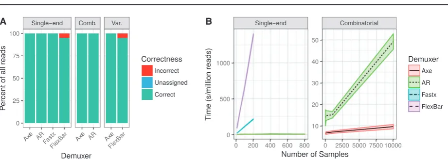
AdapterRemoval and fastx_barcode_splitter.pl (hereafter ‘fastx’). When demultiplexing read pairs with an index sequence on one read only (single-end), both axe and fastx are able to perfectly demulti-plex all reads, with no error and with no reads left unassigned. AdapterRemoval fails to assign a minuscule proportion of reads,

while flexbar mis-assigns several percent of reads (Fig. 1A). When

demultiplexing combinatorially indexed read pairs, axe again demultiplexes all reads perfectly and AdapterRemoval fails to assign a small proportion. When demultiplexing reads with variable-length index sequences, axe performs perfectly, while flexbar mis-assigns several percent of reads. In all cases, axe is the fastest demultiplexer tested. AdapterRemoval performs several times slower than axe. fastx and flexbar perform hundreds of times slower than axe and

AdapterRemoval (Fig. 1B). The methods underlying these

experi-ments are available as onlineSupplementary Material.

3.2 Summary

Here, we implement a rapid and accurate algorithm for demultiplex-ing 5’-indexed reads. We show equal or improved accuracy and reduced computational cost compared to previous software devel-oped to perform this task. In addition, more complex indexing schemes including combinatorial and/or variable length index

sequences are supported. While in-read indexing is being phased out

in some protocols, it persists in others such as GBS (Elshireet al.,

2011) and RNAseq using unique molecular identifiers (Kivioja

et al., 2012). Additionally, Axe’s algorithm is applicable to demulti-plexing out-of-read indexing schemes, though the implementation does not currently support this.

Funding

This work was supported by the Australian Research Council Centre of Excellence in Plant Energy Biology [CE140100008], and was undertaken with the assistance of resources from the National Computational Infrastructure (NCI), which is supported by the Australian Government. KDM is supported by an Australian Government Research Training Program (RTP) Scholarship.

Conflict of Interest: none declared.

References

Dodt,M.et al. (2012) FLEXBAR: flexible barcode and adapter processing for next-generation sequencing platforms.Biology,1, 895–905.

Elshire,R.J.et al. (2011) A robust, simple genotyping-by-sequencing (GBS) ap-proach for high diversity species.PLoS One,6, e19379.

Hamming,R.W. (1950) Error detecting and error correcting codes.Bell Syst. Tech. J.,29, 147–160.

Kivioja,T.et al. (2012) Counting absolute numbers of molecules using unique molecular identifiers.Nat. Methods,9, 72–74.

Peterson,B.K.et al. (2012) Double digest RADseq: an inexpensive method for de novo SNP discovery and genotyping in model and non-model species.

PLoS One,7, e37135.

Renaud,G. et al. (2015) deML: robust demultiplexing of Illumina sequences using a likelihood-based approach. Bioinformatics, 31, 770–772.

Schubert,M.et al. (2016) AdapterRemoval v2: rapid adapter trimming, identi-fication, and read merging.BMC Res. Notes,9, 88.

[image:35.595.68.529.77.242.2]

A B

Fig. 1.(A) Accuracy of read assignment. Axe is able to perfectly demultiplex all reads, as is fastx. Only flexbar incorrectly assigns reads. Note: ‘Comb.’ refers to combinatorial index sets, and ‘Var.’ refers to index sets with variable length index sequences. (B) Computational performance of demultiplexers (seconds per mil-lion reads, mean6SD). Axe is the fastest in all cases, closely followed by AdapterRemoval. fastx and flexbar are appreciably slower, especially when the number of indices is large

Axe 3925

(36)

Chapter 3 libqcpp: A C++14 sequence quality

control library

This chapter outlines a software project that aimed to implement many next-gen sequenc-ing quality control measures in a unified, reusable fashion. Libqcpp is a C++ library that presents an interface to several sequence quality control measures, including base quality measurement, read filtering, GBS-specific trimming, removal of low-coverage bases and qual-ity reporting. Trimit is a command-line interface to this library. I designed and implement Trimit and Libqcpp, devised and tested several new quality control metrics, and wrote the software paper (including the online tutorials and use cases).

This paper was accepted for publication in the Journal of Open Source Software (2017; doi: 10.21105/joss.00232). The Journal of Open Source Software is a new, peer-reviewed journal for the dissemination of novel software and algorithms to a bioinformatics audience. JOSS papers are a summary of each software tool, and articles are accepted only when soft-ware meets several requirements: validation experiments are implemented in automated tests, use cases are presented in documentation and tutorials, and code is of a high quality. The se-nior author authorises the inclusion of this manuscript in my thesis.