https://doi.org/10.5194/angeo-37-183-2019 © Author(s) 2019. This work is distributed under the Creative Commons Attribution 4.0 License.
Communica
tes
On the ion-inertial-range density-power spectra
in solar wind turbulence
Rudolf A. Treumann1,3, Wolfgang Baumjohann2, and Yasuhito Narita2
1International Space Science Institute, Bern, Switzerland
2Space Research Institute, Austrian Academy of Sciences, Graz, Austria
3Geophysics Department, Ludwig Maximilian University of Munich, Munich, Germany
Correspondence:Wolfgang Baumjohann (wolfgang.baumjohann@oeaw.ac.at) Received: 20 November 2018 – Discussion started: 5 December 2018
Revised: 14 March 2019 – Accepted: 20 March 2019 – Published: 3 April 2019
Abstract.A model-independent first-principle first-order in-vestigation of the shape of turbulent density-power spectra in the ion-inertial range of the solar wind at 1 AU is pre-sented. Demagnetised ions in the ion-inertial range of quasi-neutral plasmas respond to Kolmogorov (K) or Iroshnikov– Kraichnan (IK) inertial-range velocity–turbulence power spectra via the spectrum of the velocity–turbulence-related random-mean-square induction–electric field. Maintenance of electrical quasi-neutrality by the ions causes deformations in the power spectral density of the turbulent density fluctu-ations. Assuming inertial-range K (IK) spectra in solar wind velocity turbulence and referring to observations of density-power spectra suggest that the occasionally observed scale-limited bumps in the density-power spectrum may be traced back to the electric ion response. Magnetic power spectra re-act passively to the density spectrum by warranting pressure balance. This approach still neglects contribution of Hall cur-rents and is restricted to the ion-inertial-range scale. While both density and magnetic turbulence spectra in the affected range of ion-inertial scales deviate from K or IK power law shapes, the velocity turbulence preserves its inertial-range shape in the process to which spectral advection turns out to be secondary but may become observable under special ex-ternal conditions. One such case observed by WIND is anal-ysed. We discuss various aspects of this effect, including the affected wave-number scale range, dependence on the angle between mean flow velocity and wave numbers, and, for a radially expanding solar wind flow, assuming adiabatic ex-pansion at fast solar wind speeds and a Parker dependence of the solar wind magnetic field on radius, also the
presum-able limitations on the radial location of the turbulent source region.
1 Introduction
The solar wind is a turbulent flow with an origin in the so-lar corona. It is believed to become accelerated within a few solar radii in the coronal low-beta region. Though this awaits approval, it is also believed that its turbulence orig-inates there. Turbulent power spectral densities in the solar wind have been measured in situ at around 1 AU for several decades already. They include spectra of the magnetic field (e.g. Goldstein et al., 1995; Tu and Marsch, 1995; Zhou et al., 2004; Podesta, 2011, for reviews, among others), but with improved instrumentation also of the fluid velocity (Podesta et al., 2007; Podesta, 2009; Šafránková et al., 2013), elec-tric field (Chen et al., 2011, 2012, 2014a, b), temperature (Šafránková et al., 2016), and (starting with Celnikier et al., 1983, who already reported its main properties) also of the (quasi-neutral) solar wind density (Chen et al., 2012, 2013; Šafránková et al., 2013, 2015, 2016).
1990; Spangler and Sakurai, 1995; Harmon and Coles, 2005) mostly at solar radial distances <60R≈0.25 AU in the
in-nermost very low solar wind (0.1< βi<1; e.g. the model of
McKenzie et al., 1995) region, which is of particular interest because it is the presumable source region of the solar wind, being accessible only remotely. Solar wind turbulence gener-ated here seems to freeze1and is transported radially outward afterwards by the flow. Radio-phase scintillation of space-craft signals from Viking, Helios, and Pioneer have been used early on (Woo and Armstrong, 1979) to determine solar wind density-power spectra in the radial interval≤1 AU, report-ing mean spectral Kolmogorov slopes∼ −5/3 with a strong flattening of the spectrum near the Sun at distances<30R
where the slope flattens down to∼ −7/6= −1.1, a finding which suggests evolution of the density turbulence with solar distance. In the ISM radio scintillation, observations covered a huge range of decades, from wavelength scalesλ≈15 AU down to close to the Debye lengthλD≈50 m, suggesting an
approximate Kolmogorov spectrum over 7 decades. From re-cent in situ Voyager 1 observations of ISM electron densities (Gurnett et al., 2013) a Kolmogorov spectrum has been in-ferred down to wavelengths ofλ∼106m that is followed by an adjacent spectral intensity excess on the assumed kinetic scales for wavelengthsλ&λD(Lee and Lee, 2019).
Density fluctuations δN are generally inherent to pres-sure fluctuationsδP. From fundamental physical principles, it follows that density turbulence does not evolve by itself. Through the continuity equation, it is related to velocity tur-bulence, which in its course requires the presence of free en-ergy, being driven by external forces. It is primary, while tur-bulence in density, temperature, and the magnetic field is sec-ondary (for a different claim, see Howes and Nielson, 2013; Nielson et al., 2013). Density turbulence may signal the pres-ence of a population of compressive (magneto-acoustic-like) fluctuations in addition to the usually assumed (e.g. Biskamp, 2003; Howes, 2015) alfvénic turbulence, the dominant fluid– magnetic fluctuation family dealing with the mutually related alfvénic velocity and magnetic fields made use of in magne-tohydrodynamic (MHD) theory based on Elsasser variables (Elsasser, 1950).
Inertial-range velocity turbulence is subject to Kol-mogorov (KolKol-mogorov, 1941a, b, 1962) or Iroshnikov– Kraichnan (Iroshnikov, 1964; Kraichnan, 1965, 1966, 1967) turbulence spectra. (Regarding their generalisation to anisotropy with respect to any mean magnetic field, see
Gol-1We do not touch on the subtle question of whether any frozen
turbulence on MHD-scales above the ion-cyclotron radius in a low-beta or strong-field plasma can evolve. According to inferred spatial anisotropies, it seems that close to the Sun, turbulence in the den-sity is almost field-aligned. On the other hand, ion-inertial-range turbulence at shorter scales will be much less affected. It can be considered to be isotropic. Near 1 AU, where most in situ obser-vations take place, one hasβ&1. One may expect that turbulence here also contains contributions which are generated locally, if only some free energy would become available.
dreich and Sridhar, 1995.) In the solar wind, Kolmogorov inertial-range spectra reaching down into the presumable dis-sipation range have been confirmed by a wealth of in situ observations (e.g. Goldstein et al., 1995; Tu and Marsch, 1995; Zhou et al., 2004; Alexandrova et al., 2009; Boldyrev et al., 2011; Matthaeus et al., 2016; Lugones et al., 2016; Podesta, 2011; Podesta et al., 2006, 2007; Sahraoui et al., 2009, and others). Since the mean fieldsB0, T0, N0, U0
them-selves obey pressure balance, one has the following for pres-sure balance among the turbulent fluctuations:
h|δB|2i B02
= p
h|δN|2i
N0
+ p
h|δT|2i
T0
. (1)
The angular bracketsh. . .iindicate averaging over the spatial scales of the turbulence with respect to turbulent fluctuations. Alfvénic fluctuations (e.g. Howes, 2015, for a recent theoreti-cal account of their importance in MHD turbulence) compen-sate separately due to their magnetic and velocity fluctuations being related; they do not contribute to extra compression. In order to infer the contribution of density fluctuations, one compares their spectral densities with those of the tempera-tureδT or magnetic fieldδB. This requires normalisation to the means. Solar wind densities at 1 AU are of the order of N0∼10 cm−3, while ion thermal speeds are of the order of
vi∼30 km s−1. Moreover, mean plasma betas are of the
or-der ofβi∼1 here. For checking pressure balance, measured
density fluctuations can be compared with those two. An example is shown in Fig. 1 based on solar wind mea-surements on 6 July 2012 (Šafránková et al., 2015, 2016). There is not much freedom left in choosing the mean densi-ties and temperatures in Fig. 1. Densidensi-ties at 1 AU barely ex-ceed 10 cm−3. Electron temperatures are insensitive to those low-frequency density fluctuations. High mobility makes electron reaction isothermal.
The data in Fig. 1 show the relative dominance of density fluctuations over ion temperature fluctuations under mod-erately low-speed solar wind conditions at all frequencies larger than the lowest accessible MHD frequencies. This is not surprising because one would not expect large temper-ature effects. Ion heating is a slow process which does not react to any fast pressure fluctuations caused by density or magnetic turbulence. It just shows that the turbulent thermal pressure is mainly due to density fluctuations over most of the frequency range. In the low-frequency MHD range the kinetic pressure of large-scale turbulent eddies dominates.
Figure 1.Normalised solar wind power spectra of turbulent temper-ature and density fluctuations. The curves are based on data from Šafránková et al. (2016) obtained on 6 July 2012 from the Bright Monitor of the Solar Wind (BMSW) instrument aboard the Spektr-R spacecraft. The solar wind conditions of these observations have been tabulated (Chen et al., 2014a). They indicate rather slow com-pared to medium conditions. The data have been rescaled and nor-malised to the main densityN0and temperatureT0in order to show
their relative contributions to an assumed solar wind pressure bal-ance. The interesting result is that in the lowest MHD frequency range density fluctuations are irrelevant with respect to pressure bal-ance. At higher frequencies, however, the density fluctuations dom-inate the temperature fluctuations.
suggested to indicate the presence of kinetic Alfvén waves which may be excited in the Hall-MHD (e.g. Huba, 2003) range as eigenmodes of the plasma. Models including Alfvén ion-cyclotron waves (Harmon and Coles, 2005) or kinetic Alfvén waves (Chandran et al., 2009) have been proposed to cause spectral flattening. Kinetic Alfvén waves may also lead to bumps if onlyβi1. In fact, kinetic Alfvén waves
possess a large perpendicular wave numberk⊥λi∼1 of the
order of the inverse ion-inertial length (e.g. Baumjohann and Treumann, 1996), the scale on which ions demagnetise. If sufficient free energy is available, they can thus be excited and propagate in this regime (e.g. Gary, 1993; Treumann and Baumjohann, 1997). Recently Wu et al. (2019) provided kinetic-theoretical arguments for kinetic Alfvén waves con-tributing to turbulent dissipation in the ion-inertial scale re-gion. Causing bumps, the waves should develop large am-plitudes on the background of general turbulence, i.e. caus-ing intermittency. This requires the presence of a substan-tial amount of unidentified free energy, for instance in the form of intense plasma beams, which are very well known in relation to collisionless shocks both upstream and down-stream (e.g. Balogh and Treumann, 2013). If kinetic Alfvén waves are unambiguously confirmed (see, e.g. Salem et al., 2012), the inner solar wind at.0.6 AU could be subject to the continuous presence of small-scale collisionless shocks, a assumption that is not unreasonable and which would be
supported by observation of sporadic nonthermal coronal ra-dio emissions (type I through type IV solar rara-dio bursts).
In the present note we take a completely different model-independentpoint of view, avoiding reference to any super-imposed plasma instabilities or intermittency (e.g. Chen et al., 2014b). We do not develop any “new theory” of turbu-lence. Instead, we remain in the realm of turbulent fluctu-ations, asking for the effect of ion inertia, with respect to ion demagnetisation in the ion-inertial Hall-MHD range, on the shape of the inertial-range power spectral density which will be illustrated referring to a few selected observations. To demonstrate pressure balance we refer to related mag-netic power spectra, both measured in situ aboard spacecraft, which require a rather sophisticated instrumentation. Those measurements were anticipated by indirectly inferred den-sity spectra in the solar wind (Woo, 1981; Coles and Fil-ice, 1985; Bourgeois et al., 1985) and the interstellar plasma (Coles, 1978; Armstrong et al., 1981, 1990) from detection of ground-based radio scintillations.
In the next section we discuss the response of demagne-tised ions to the presence of turbulence on scales between the ion and electron inertial lengths. We interpret this response as the consequence of electric field fluctuations in relation to the turbulent velocity field. The requirement of charge neu-trality maps them to the density field via Poisson’s equa-tion. The additional contribution of the Hall effect can be separated. We then refer to turbulence theory, assuming that the mechanical inertial-range velocity–turbulence spectrum is either Kolmogorov (K) or Iroshnikov–Kraichnan (IK) and, in a fast-streaming solar wind under relatively weak condi-tions (Treumann et al., 2019), maps from wave number k into a stationary observer’s frequencyωs space via Taylor’s
hypothesis (Taylor, 1938).
In order to be more general, we split the mean flow veloc-ity into bulkV0and large-eddyU0velocities, the latter being
known (Tennekes, 1975) to cause Doppler broadening of the local velocity spectrum at a fixed wave number (reviewed and backed by numerical simulations by Fung et al., 1992; Kaneda, 1993). Imposing the theoretical K or IK inertial-range spectra, we then find the deformed power density spec-tra of density turbulence versus spacecraft frequency. We ap-ply these to some observed spectral density bumps which we check on a measured magnetic power spectrum for pressure balance. The results are tabulated. Since bumpy spectra are rather rare, we also consider two more “normal” bumpless spectra. Such deformed density-power spectra which exhibit some typical spectral flattening were obtained under differ-ent solar wind conditions. The paper concludes with a brief discussion of the results.
2 Inertial-range ion response
spectra, in particular their deviation from the expected mono-tonic inertial-range power law decay towards high wave numbers prior to entering the presumable dissipation range.
The philosophy of our approach is the following. Turbu-lence is always mechanical, i.e. in the velocity. It obeys a turbulent spectrum which extends over all scales of the turbu-lence. In a plasma, containing charged particles of different mass, these scales for the particles divide into magnetised, inertial, unmagnetised, and dissipative groups. On each of these intervals, the particles behave differently, reacting to the turbulence in the velocity. In the inertial range, the par-ticles lose their magnetic property. They do not react to the magnetic field. They, however, are sensitive to the presence of electric fields, independent of their origin. Turbulence in velocity in a conducting medium in the presence of exter-nal magnetic fields is always accompanied by turbulence in the electric field due to gauge invariance, namely the Lorentz force. This electric field affects the unmagnetised component of the plasma, the ions in our case, which to maintain quasi-neutrality tend to compensate it. Below we deal with this ef-fect and its consequences for the density-power spectrum. 2.1 Electric field fluctuations in the ion-inertial range
The steep decay of the normalised fluctuations in ion tem-perature above frequencies >10−1Hz is certainly due to the drop in ion dynamics at frequencies close to and ex-ceeding the ion-cyclotron frequency, which at 1 AU distance from the Sun is of the order of fci=ωci/2π∼1 Hz for a
nominal magnetic field of ∼10 nT. In this range we en-ter the (dissipationless) ion-inertial or Hall (electron-MHD) domain where ions demagnetise, currents are carried by magnetised electrons, both species decouple magnetically, and Hall currents arise. At those frequencies, far below the electron fe=ωe/2π∼35 kHz and (assuming protons) ion
fi=ωi/2π∼0.8 kHz plasma frequencies, ions and
elec-trons couple mainly through the condition of quasi-neutrality, i.e. via the turbulent induction–electric field which becomes2 δE= −δV⊥×B0−(V0+U0)×δB−
− 1
eN0
B0×δJ+
+DδV×δB+ 1 eN0
δJ×δN N0
B0−δB E
. (2)
For later use, we split the main velocity fieldhVi =V0+U0
into the bulk flow (convection)V0and an advection veloc-2This equation is easily obtained by standard methods when
splitting the fields in the ideal (collisionless) Hall-MHD Ohm’s law:
E= −V×B+(1/eN )J×B, withE,B,V ,Jelectric, magnetic, and current fields, into mean (index 0) and fluctuating fields accord-ing toE=E0+δEetc.; averaging over the fluctuation scales, with
h. . .iindicating the averaging procedure, yields the mean-field elec-tric field equation. Subtracting it from the original equation pro-duces the wanted expression of the turbulent electric fluctuations
δEthrough the mean and fluctuating velocity and magnetic fields.
ityU0. The latter is the mean velocity of a small number of
large eddies which carry the main energy of the turbulence. Even for stationary turbulence, they advect the bulk of small-scale eddies around at speedU0(Tennekes, 1975; Fung et al.,
1992).
The last three averaged nonlinear terms within the angu-lar bracketsh. . .ion the right are the nonlinear contributions of the fluctuations to the mean fields yielding an electromo-tive force which contributes to mean-field processes like con-vection, dynamo action, and turbulent diffusion. They vary only on the large mean-field scale. On the fluctuation scale they are constant and can be dropped, unless the turbulence is bounded, in which case boundary effects must be taken into account at the large scales of the system. Generally, in the solar wind this is not the case. The remaining three linear terms distinguish between directions parallel and perpendic-ular to the main magnetic fieldB0. The third linear term is
the genuine perpendicular Hall contribution. From Ampere’s law for the current fluctuationµ0δJ = ∇ ×δBwe have the
following for the perpendicular and parallel components of the turbulent electric field:
δE⊥=B0× h
δV⊥−
U0k
B0
δB⊥−
− 1
eµ0N0
∇ ×δB ⊥
i
−U0⊥×δBk
δEk= −U0⊥×δB⊥ ==H⇒ 0. (3)
The second of these equations is of no interest, because the low-frequency parallel electric field its right-hand side produces is readily compensated by electron displacements alongB0.
This leaves us with the fluctuating perpendicular induc-tion field in the first Eq. (3). Here, any parallel advec-tionU0kattributes to the perpendicular velocity fluctuations
from perpendicular magnetic fluctuationsδB⊥. On the other
hand, any present parallel compressive magnetic fluctuations δBk=B0(δBk/B0)contribute through perpendicular
advec-tionU0⊥. In their absence, when the magnetic field is
non-compressive, the last term disappears.
The complete Hall contribution to the electric field, viz. the last term in the brackets in Eq. (3), can be written as
δEH⊥= − B0 eµ0N0
∇⊥δBk− ∇kδB⊥
. (4)
Even forU0k=0, it contributes through the turbulent
fluc-tuations in the magnetic field. As both these contributions depend only onδB, we can isolate them for separate consid-eration. One observes that, in the absence of any compressive magnetic componentsδBkand homogeneity along the
2.2 Relation to density fluctuations: Poisson’s equation
Let us assume that advection by large-scale energy-carrying eddies is perpendicular U0=U0⊥, and there are no
com-pressive magnetic fluctuations δBk=0. In Eq. (2) this
re-duces to considering only the first term containing the ve-locity fluctuations. We ask for its effect on the density fluc-tuations in the ion-inertial domain on scales where the ions demagnetise.
On scales in the ion-inertial range shorter than either the ion thermal gyroradius ρi=vi/ωci or – depending on
the direction to the mean magnetic field B0 and the value
of plasma beta β=2µ0N0T0/B02, with ωci=eB0/mi
ion-cyclotron and ωi=e
√
N0/0mi ion plasma frequency,
re-spectively – inertial lengthλi=c/ωi, the ions demagnetise.
Being non-magnetic, they do not distinguish between poten-tial and induction–electric fields. They experience the induc-tion field caused by the spectrum of velocity fluctuainduc-tions as an external electric field which, in an electron-proton plasma, causes a charge density fluctuationeδNi=eδNeand thus a
density fluctuationδN. Poisson’s equation implies that ∇ ·δE= e
0
δN ==H⇒ ik·δEk=
e 0
δNk. (5)
The right expression is its Fourier transform. For complete-ness we note that the Hall contribution to the Poisson equa-tion in Fourier space reads
ik⊥·δEH⊥k=
B0
eµ0N0
k⊥2δBkk−kkk⊥·δB⊥k
= e
0
δNkH. (6) Again it becomes obvious that absence of parallel (compres-sive) magnetic turbulence eliminates the first term in this expression, while purely perpendicular propagation elimi-nates the second term. Alfvénic turbulence, for instance, with δBk=0 and k⊥=0, has no Hall effect on the modulation
of the density spectrum, a fact which is well known. On the other hand, for perpendicular wave numbersk=k⊥only
compressive Hall-magnetic fluctuationsδBkk⊥ contribute to
the Hall fluctuations in the densityδNkH⊥.
2.3 Relation between density and velocity power spectra
We are interested in the power spectrum of the turbulent den-sity fluctuations in the proper frame of the turbulence.
Multiplication of the only remaining first term in the elec-tric induction field Eq. (3) with wave number k selects wave numbersk⊥perpendicular toB0. The combination of
Eq. (2) and the Poisson equation then yields an expression for the power spectrum of the turbulent density fluctuations3 in wave-number space
h|δN|2ik⊥= 0B0
e 2
k⊥2h|δV|2ik⊥, (7)
3The procedure of obtaining the power spectrum is standard, so
we skip the formal steps which lead to this expression.
where we from now on drop the index ⊥ on the velocity δV⊥. Angular brackets again symbolise spatial averaging
over the fluctuation scale. The functional dependence on the wave number is indicated by the indexk⊥. It is obvious that
the power spectrum of density fluctuations in the ion-inertial Hall-MHD domain is completely determined by the power spectrum of the turbulent velocity4. This can be written as h|δN|2ik⊥
N02
=VA c
2k⊥ ωi 2
h|δV|2ik⊥
=h|δV|
2i
k⊥
c2
VA c
2 k⊥λi
2
, (8)
whereVA2=B02/µ0miN0 is the squared Alfvén speed, and
ωi2=e2N0/0miis the squared proton plasma frequency. As
expected, in order to contribute to density fluctuations, per-pendicular scalesλ⊥< λismaller than the ion-inertial length
λi=c/ωi are required, while in the long-wavelength range
k⊥λi<1, there is no effect on the spectrum. This is in
agree-ment with the assumption that any spectral modification is expected only in the ion-inertial range.
The last equation is the main formal result. It is the wanted relation between the power spectra of density and velocity fluctuations. It contains the response of the unmagnetised ions to the mechanical turbulence.
2.4 Affected scale range
The density response demands that the ions are unmag-netised. This implies that k⊥ρi<1, where ρi=vi/ωci=
λivi/VA is the ion gyroradius, withvias the thermal speed.
Thus we have two conditions which must simultaneously be satisfied:
k⊥λi>1 and k⊥λi>
VA
vi
≡β− 1 2
i . (9)
ForVA< vithe second condition is trivial. This is, however,
a rare case, so the more realistic restriction is the opposite small ion-beta case whenVA> viand henceβi<1. It must,
however, be combined with another condition which requires that the wave numbers be smaller than the inverse electron gyroradiusρe=ve/ωce. The relation between ρe andρi is
ρe2/ρi2=meTe/miTi. Moreover we haveρi/λi=vi/VA, and
in addition, βi=v2i/VA2=(Ti/Te)βe. Using all these
rela-tions, we obtain finally that 1< k⊥2λ2iβi<
mi
me
Ti
Te
for βi<1. (10)
4One may object that, at smaller wave numbers outside the
ion-inertial range, this would also be the case, which is true. There, reference to the continuity equation, for advection speedsU06=0,
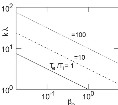
Figure 2.The range of permitted values ofk⊥λias function ofβe
for different ratiosTe/Ti. Only the range above the lines is relevant.
In the solar wind, usuallyTe> Ti, implying thatβe> βi(Newbury
et al., 1998; Wilson III et al., 2018) unless the electrons become cooled by some process like emitting radiation, electron hole for-mation, or charge exchange.
This expression defines the marginal condition for the exis-tence of a range in wave numbers where the ions respond to the spectrum of the turbulent electric fieldδE:
Ti
Te&
me
mi
∼0.001. (11)
Because of the smallness of the right-hand side, this is a weak restriction. As expected, any effect on the density-power spectrum will disappear at wave numbers k⊥ρe where the
electrons demagnetise. On the other hand, the lower wave-number limit is a sensitive function of the external condi-tions. This becomes clear when writing it in the form Te/Tiβe< k2⊥λ
2
i. (12)
The electron plasma beta in the solar wind is of the order of βe&O(1). However, the temperature ratioTe/Ti is variable
and usually large, varying between a few and a few tens. Thus usuallyβi<1. Figure 2 shows a graph of this dependence.
2.5 Application to K and IK inertial-range models of turbulence
The power spectrum of the Poisson-modified ion-inertial-range density turbulence can be inferred once the power spectral density of the velocity is given. This spectrum must either be known a priori or requires reference to some model of turbulence.
We do not develop any model of turbulence here. In appli-cation to the solar wind we just make us, in the following, of the Kolmogorov (K) spectrum (or its anisotropic extension by Goldreich and Sridhar, 1995, abbreviated KGS) but will
also refer to the IK spectrum, which both have previously been found to be of relevance in solar wind turbulence.
We shall make use of those spectra in two forms: the original ones which just assume stationarity and absence of any bulk flows and their modified advected extensions. The latter account for a distinction between a small number of large energy-carrying eddies with mean eddy vortex speed U0and bulk turbulence consisting of large numbers of small
energy-poor eddies which are frozen to the large eddies. The large eddies stir the small-scale turbulence, forcing it into
advective motion (Tennekes, 1975). This causes a Doppler broadening of the wave-number spectrum at fixedkand has been confirmed by numerical simulations (Fung et al., 1992; Kaneda, 1993). Below, it will be found that this advection cannot be resolved in bulk convective flow which buries the subtle effect of Doppler broadening. A probable counterex-ample is shown in Fig. 5.
The stationary velocity spectrum of turbulent eddies at en-ergy injection rateexhibits a broad inertial power law range ink(Kolmogorov, 1941a, b, 1962; Obukhov, 1941) which, between injectionkin and dissipation atkd wave numbers,
obeys the famous isotropic Kolmogorov power spectral den-sity law in wave-number space:
δV
2
k≡EK(k)=CK
2 3k−
5
3 for kin< k < kd, (13) withCK≈1.65 as Kolmogorov’s constant of
proportional-ity (as determined by Gotoh and Fukayama, 2001, using nu-merical simulations). Clearly, in a fast-streaming solar wind, when straightforwardly mapping this K spectrum by the Tay-lor hypothesis (TayTay-lor, 1938) into the stationary spacecraft frame, the spectral index is unchanged, and one trivially re-covers theω−
5 3
s Kolmogorov slope in frequency space.
This changes drastically when referring to an advected K spectrum of velocity turbulence (Fung et al., 1992; Kaneda, 1993) which yields the above-mentioned spectral Doppler broadening at fixedk,
Ekωad
k=
1 2
EK(k)
√ 2π kU0
X
±
exph−1 2
ω±2 (kU0)2
i ,
ω±=ωk±`Kk
2
3, (14)
which is due to decorrelation of the small eddies in advec-tive transport, with `K∼O(1) being some constant. The
k23 dependence in the argument of the exponential results from advection k·δV of neighbouring eddies at velocity ofδV ∝k−13 (Tennekes, 1975; Fung et al., 1992). The fre-quencyωk stands for the internal dependence of the
turbu-lent frequency on the turbuturbu-lent wave numberk. It can be un-derstood as an internal “turbulent dispersion relation”, which is neglected in turbulence theory.5Then the advected power
5The notion of a turbulent dispersion relation is alien to
Figure 3. Solar wind power spectra of turbulent density fluctua-tions (based on BMSW data from Šafránková et al., 2013, obtained on 25 October 2011). Single point measurements were obtained with six Faraday cups with time resolution of 31 ms (∼30 Hz) un-der the following solar wind conditions: densityN∼3×10⁶m−3, mean magnetic fieldB0∼8 nT, bulk speedV0∼540 km s−1, ion
temperature Ti∼10 nT, Alfvén Mach numberMA∼6, and total β∼0.3, implying dilute lowβ(highMA) and moderately fast flow
conditions. The local thermal ion gyroradius isρi∼2.2×10⁴m.
The vertical line indicates the local ion-cyclotron frequencyfci= ωci/2π≈0.15 Hz. Plasma frequency isfi=ωi/2π≈400 Hz.fm
andfMare the approximate minimum and maximum frequencies
of the bumpy range, respectively. The data were averaged over
∼1200 s measuring time and subsequently filtered (cf. Šafránková et al., 2016, for the description of the data reduction). The spec-trum shown is the average specspec-trum with line width roughly corre-sponding to the largest spread of the filtered data in the logarithmic ordinate direction and applied to the whole spectrum. The power spectrum exhibits a (so-called) bump at intermediate frequencies
of positive slopes∼ω13 or∼ω12. This is in agreement with it
be-ing caused by the response of the non-magnetic ions to the elec-tric induction field of the turbulent mechanical fluctuations in the solar wind velocity in Kolmogorov (K; solid line) or Iroshnikov– Kraichnan (IK; dashed line) inertial-range turbulence. The large scatter in the data (weight of line) inhibits distinguishing between K and IK inertial-range velocity turbulence.
collecting any temporal changes under the loosely defined term in-termittency. However, observation of stationary turbulence shows that eddies come and go on an internal timescale, which station-ary theory integrates out. In Fourier representation this corresponds to an integration of the spectral density S(ωk,k)with respect to
frequencyωk (e.g. Biskamp, 2003), which leaves only the
wave-number dependence. The spectral densityS occupies a volume in
(ω,k)space. Resolved forω=ωk(k), it yields a complex multiply
spectrum at largekis power law
Ekωad
k∝
EK(k)
k exp
−1 2cos
2γ
k
∼k−83, (15)
ω±≈k·U0=kU0cosγk. (16)
In the stationary turbulence frame the power spectrum of turbulence in the velocity decays to ∝k−83 with non-Kolmogorov spectral index 8/3≈2.7.
It is of particular interest to note that solar wind turbu-lent power spectra at high frequency repeatedly obey spectral indices very close to this number. Boldly referring to Tay-lor’s hypothesis whereωs∝k, one might conclude then that
a convective flow maps this spectral range of the advected turbulent K spectrum into the spacecraft frame where it ap-pears as anω−
8 3
s spectrum.
If this is true, then the corresponding observed spec-tral transition (or break point) from the specspec-tral K index ∼5/3 to the steeper index∼8/3 observed in the wave-number power spectra indicates the division between large-scale energy-carrying, energy-rich turbulent eddies and the bulk of energy-poor small-scale eddies in the mechanical tur-bulence. It thus provides a simple explanation of the change in spectral index from∼5/3 (K spectrum) to.3 (advected K turbulence spectrum) without invoking any sophisticated turbulence theory as well as having no effects of dissipation. Inspecting the behaviour in the long-wavelength range, one finds that the exponential dependence exp(−`2K/U02k23) suppresses the spectrum here. This flattens the inertial-range spectrum towards small wave numberskininto the large-eddy
range where it causes bending of the spectrum. The wave number at spectral maximum is
kmin.`3K/16U03 √
2. (17)
Approaching from the Kolmogorov inertial range towards a smallerk, one observes flattening untilkmin< kin. In most
cases this point will lie outside the observation range. In the stationary turbulence frame the frequency spec-trum is obtained when integrated with respect tok(Biskamp, 2003). It then maps the Doppler broadened advected veloc-ity power spectrum (Fung et al., 1992; Kaneda, 1993) to the Kolmogorov law in the source-region frequency space:
kd
Z
kin
dkEad
kωk∼E
ad
K(ω) ∝ ω
−53. (18)
connected surface, the turbulent dispersion relation, which has noth-ing in common with a linear dispersion relation resultnoth-ing from the solution of a linear eigenmode wave equation. It contains the depen-dence of Fourier frequencyωk on Fourier wave numberk. Though
This mapping is independent of Taylor’s hypothesis. It strictly applies only to the turbulent reference frame. When attempting to map it into the spacecraft frame via Taylor’s Galilei transformation, referring to solar wind flow at finite V06=0, one must return to its wave-number representation in
Eq. (14). This transformation, though straightforward, is ob-scured by the appearance ofkin the exponential throughω±.
According to Taylor the turbulence frame frequency trans-forms as
ωk=ωs−kV0cosα. α=6 (k,V0). (19)
This is Taylor’s Galilei transformation. Neglecting ωk
im-plies thatωs=kV0cosα. The exponential reduces to
exph−1 4
ωk+kV0cosα±`Kk 2 3
kU0
2i
= (20)
=exph− 1 4(kλi)
2 3
λ 1 3
i `K
U0 2i
(21)
−→1− 1 4(kλi)
2 3
λ 1 3
i `K
U0 2
, (22)
with λ 1 3
i `/U0≡U`K/U0 being a velocity ratio. The arrow
holds for the ion-inertial rangekλi>1 andU`K/U0<1. The
exponential expression leads to an advected K spectrum as observed by the spacecraft in frequency space:
Eωads ∝ω− 8 3
s exp h
−1 4
V0cosα ωsλi
23UK
`
U0 2i
, (23)
which, as before for large ωs, is of the spectral index 8/3.
With decreasing spacecraft frequency ωs, the exponential
correction factor acts to suppress the spectrum. This corre-sponds to a spectral flattening towards smallerωs. It might
even cause a spectral dip, depending on the parameters and velocities involved. The effect is strongest for aligned streaming and the eddy wave number. For α∼90◦ one re-covers the index 8/3.
It is most interesting that spectral broadening, when trans-formed into the spacecraft frame in streaming turbulence, causes that strong of a difference between the original Kol-mogorov and the advected KolKol-mogorov spectrum. This spec-tral behaviour is still independent of the Poisson modifica-tion, which we are going to investigate in the next section.
3 Ion-inertial-range density-power spectrum
Here we apply the Poisson-modified expressions to the the-oretical inertial-range K and IK turbulence models. We con-centrate on the inertial-range K spectrum and rewrite the re-sult subsequently to the IK spectrum.
3.1 Inertial-range K and IK density-power spectrum
For the simple inertial-range K spectrum, we know from Eqs. (7) and (13) that
h|δN|2ik⊥=CK 0B0
e 2
23k 1 3
⊥ for k⊥in< k⊥< k⊥d.
(24) This is a very simple wave-number dependence of the power spectrum of density turbulence, permitting (Treumann et al., 2019) Taylor’s Galilei transformation into the spacecraft frame. Settingk⊥=ωs/V0cosαwe immediately obtain
h|δN|2ik⊥∝ ω 1 3
s, (25)
with factor of proportionalityCK(0B0/e)2(2/V0cosα)
1 3. Following exactly the same reasoning when dealing with the IK spectrum, which has power index 3/2, we obtain h|δN|2ik⊥∝ ω
1 2
s. (26)
Hence, the effect of the Poisson response of the plasma to the inertial-range power spectra of K and IK turbulence in the velocity is to generate a positive slope in the density-power spectrum when transformed by Taylor’s Galilei transforma-tion into the spacecraft frame.
We now proceed to the investigation of the effect of advec-tion.
3.2 Advected Poisson-modified spectrum atV0=0
Use of the advected power spectral density Eq. (14) of the velocity field forV0=0 in the transformed Poisson
equa-tion, withk→k⊥being perpendicular to the mean magnetic
fieldB0, yields the following for the non-convected advected
turbulent ion-inertial-range Poisson-modified density-power spectrum in the stationary large-eddy turbulence frame:
h|δN|2iadω
kk⊥=
02B02 e2 k
2
⊥h|δV|2iωkk⊥
=
2 0B02
e2 k 2 ⊥E
ad
k⊥ωk
∝k− 2 3
⊥ X
±
exph−1 2
ω2± (kU0)2
i
. (27)
Integration with respect tok⊥under the above assumption on
ω±≈k⊥U0yields the following for the Eulerian (Fung et al.,
1992) density-power spectrum in frequency spaceω`< ω <
ωuin the ion-inertial domain of the turbulent inertial range:
h|δN|2iadω ∼ ω13, k 2 3
ir
1
3 =ω`< ω < ωu. (28)
2π ωi/c(or 2π vi/ωci) is the wave number presumably
corre-sponding to the lower end of the ion-inertial range. The up-per bound on the frequencyωuremains undetermined. One
assumption would be thatωu is the lower-hybrid frequency
which is intermediate to the ion and electron cyclotron fre-quencies. At this frequency electrons become capable of dis-charging the electric induction field, thus breaking the spec-trum to return to its Kolmogorov slope at increasing fre-quency.
In contrast to the Kolmogorov law, thePoisson-mediated proper advecteddensity-power spectrum Eq. (28) increases with frequency in the proper stationary frame of the turbu-lence. This increase is restricted to that part of the inertial K range which corresponds to the ion-inertial scale and fre-quency range.
The case of an IK spectrum leads to an advected velocity spectrum
h|δV|2iω
kk⊥∝k
−32
⊥ , (29)
which yields
h|δN|2iad
ωkk⊥∝k
−1
2
⊥ X
±
exph−1 2
ω±2
(kU0)2 i
,
ω±=ωk±`IKk
3 4
⊥. (30)
Integration with respect tok⊥then gives the proper advected
frequency spectrum in the stationary frame of IK turbulence:
h|δN|2iadω ∼ ω12. (31)
This proper IK density spectrum increases with frequency like the root of the proper frequency.
3.3 Taylor’s Galilei-transformed Poisson-modified advected spectra
Turning to the fast-streaming solar wind, we find that with k⊥=ωs/V0cosα for the Poisson-modified advected and
convected K density spectrum,
h|δN|2iKω,ad s ∝ω
−2
3
s exp h
−1 4
V0cosα ωsλi
23UK
`
U0 2i
, (32) where we again neglected the proper frequency dependence. This Taylor’s Galilei-transformed density spectrum decays with increasing frequency, albeit at a weak power∼2/3. At large frequency ωs the exponent is 1, and the spectrum
be-comes∝ω− 2 3
s . Towards smallerωsthe spectrum flattens and
assumes its maximum at ωsmK =3
8
V0cosα λi
UK
`
U0 3
. (33)
[image:9.612.309.554.65.306.2]The same reasoning produces, for the Poisson-modified advected IK spectrum, the Taylor’s Galilei-transformed
Figure 4.Solar wind power spectra of the turbulent magnetic field for the same time interval as in Fig. 3 measured by the WIND space-craft (data from Šafránková et al., 2013), which was located at the Lagrange point L1. Line width accounts for the scatter of data. The magnetic turbulence spectrum exhibits a deformation similar to that in the density-power spectrum and the same frequency interval. The positive slope∼ω16 in the deformation confirms its origin from pressure balance. It indicates its nature being secondary to turbu-lence in density. The solid (dashed) line corresponds to an K (IK) velocity spectrum. The scatter of data was again substantial, thus inhibiting distinction between the two cases.
spacecraft frequency spectrum
h|δN|2iIKω,ad s ∝ω
−12 s exp
h −1
4
V0cosα ωsλi
34UIK
`
U0 2i
. (34) Both advected K and IK spectra have negative slopes in spacecraft frequencyωs. Like in the case of a K spectrum,
this spectrum approaches its steepest slope of 1/2 at large spacecraft frequenciesωs, while in the direction of small
fre-quencies, it flattens out to assume its maximum value at ωmIK=7
8
V0cosα
λi
32UIK
`
U0 3
. (35)
maxima only if these maxima are still in the inertial range of the advected K or IK spectrum. Only in this case does the spacecraft frequency spectrum exhibit a bump at their nominal maximum frequencies ωsm. When the maximum
frequency falls outside the ion-inertial range the bump will be absent, while the spectrum will be flatter than at large frequencies. Such flattened bumpless spectra have been ob-served. The next subsections provide examples of observed bumpy and bumpless spectra in the spacecraft frequency frame.
4 Application to selected observations in the solar wind
In the following two subsections we apply the above theory to real observations made in situ in the solar wind. We first consider density-power spectra exhibiting well-expressed spectral bumps of positive slope. We then show two examples where no bump is present but where the power spectra ex-hibit a scale-limited excess and consequently a scale-limited spectral flattening.
4.1 Observed bumpy solar wind power spectra of turbulent density
Figure 3 is an example of a density spectrum with respect to spacecraft frequency which exhibits a positive slope (or bump) on the otherwise negative slope of the main spectrum. The data in this figure were taken from published spectra (Šafránková et al., 2013) in the solar wind at an average bulk velocity ofV0≈534 km s−1, densityN0≈3×10⁶m−3, and
magnetic field B0≈8 nT, yielding a super-alfvénic Alfvén
Mach number MA≈6, ion temperatureTi.3 eV, and total
plasma β≈0.3, i.e. low-beta conditions. The straight solid and broken lines drawn across this slope correspond to the predicted ∼ω13K and ∼ω12 IK slopes under convection-dominated conditions. Both these lines fit the shape very well though it cannot be decided which of the inertial-range tur-bulence models provides a better fit, as the large scatter of the data mimicked by the line width inhibits any distinction. It is however obvious from Table 1 that advection plays no role in this case.
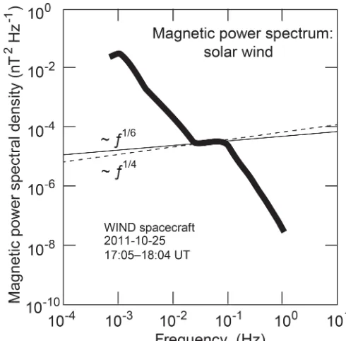
In order to check pressure balance between the density and magnetic field fluctuations, we refer to turbulent magnetic power spectra obtained at the WIND spacecraft Šafránková et al. (2013). WIND was located in the L1 Lagrange point. Magnetic field fluctuations were related in time to the Bright Monitor of the Solar Wind (BMSW) observations by the so-lar wind flow. In spite of their scatter, the data were suf-ficiently stationary for comparison to the density measure-ments.
Figure 4 shows the WIND magnetic power spectral den-sities. For transformation of the point cloud into a continu-ous line, we applied the same technique (Šafránková et al., 2016) as that for the density spectrum. The spectrum
ex-Table 1.K and IK ion-inertial-range spectral indicesk−a,k−(a−2),
ωsb, andEBs∼ωb/s 2without and with advection.
h|δV|2i a a−2 b b/2
EK 53 −13 13 16 Ead
K
8 3
2
3 −
2
3 −
1 3 EIK 32 −12 12 14 EIKad 52 12 −1
2 −
1 4
hibits the expected positive slope in the BMSW frequency interval. The straight solid and broken lines along the posi-tive slope correspond (within the uncertainty of the observa-tions) to the root slopes of K and IK density inertial-range spectra h|δB|2iω
s∼ω 1 6
s and ∼ω
1 4
s, respectively. The
mag-netic spectrum is the consequence of the K or IK density spectrum∼ω
1 3
s and∼ω
1 2
s, respectively. Fluctuations in
tem-perature do not, within experimental uncertainty, play any susceptible role. Comparing absolute powers is inhibited by the ungauged differences in instrumentation. (One may note that power spectral densities are positive definite quantities. Measuring their slopes is sufficient indication of pressure balance. Detailed pressure balance can only be seen when checking the phases of the fluctuations. Density and mag-netic field would then be found in the antiphase.)
4.2 The normal case: flattened density-power spectra without bump
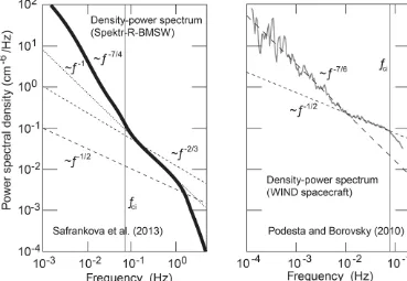
The majority of observed density-power spectra in the so-lar wind do not exhibit positive slopes. Such spectra are of monotonic negative slope. In this sense they are normal. They frequently possess break points in an intermediate range where the slopes flatten. Two typical examples are shown in Fig. 5, combined from unrelated BMSW and WIND data (Šafránková et al., 2013; Podesta and Borovsky, 2010).
Their flattened spectral intervals each extend roughly over 1 decade in frequency. The BMSW spectrum is shifted by 1 order of magnitude in frequency to higher frequencies than the WIND spectrum. Its low-frequency part below the ion-cyclotron frequency f < fci has slope ∼ω−
7
4, close to a K spectrum∼ω−53. The slope of the flat section is ∼ω−1 which is about the same as the slope of the entire low-frequency WIND spectrum before its spectral break. None of the Poisson-modified K or IK spectral slopes fit these flat-tened regions. At higher frequencies the BMSW spectrum steepens and presumably enters the dissipative range.
[image:10.612.358.498.101.183.2]space-Figure 5. Two (redrawn on same scale) cases of normal solar wind density-power spectra measured by Spektr-R-BMSW (Šafránková et al., 2013) on 10 November 2011 and WIND (Podesta and Borovsky, 2010) on 4–8 January 1995 at different solar wind conditions. BMSW observations of 2011 were obtained under low-speed (∼370 km s−1) moderately large totalβ=βi+βe∼2.5, high Alfvénic Mach
numberMA∼10, and mean-fieldB0∼5 nT conditions. Density and temperature amounted toN0∼5×10⁶m−3andTi∼10 eV, with
ion-cyclotronfci∼0.08 Hz and plasmafi∼500 Hz frequencies. WIND observations in L1 were obtained under high speed (∼640 km s−1), βi.1,B0∼6 nT,N0∼3.5×10⁶m−3,Ti∼20 eV, andMA∼9 conditions with similar cyclotron and plasma frequencies. In contrast to Fig. 3 these spectra do not exhibit regions of positive slope. Their spectral slope is interrupted by a flattened region. They share a range of spectral index∼ −1, though in different frequency intervals, while the WIND spectrum exhibits a higher-frequency range of flat slope
∼ −1/2 which is absent in the BMSW spectrum.
craft frequencies. The pronounced ω−1 spectrum at lower frequencies remains, however, unexplained for both space-craft.
When crossing the cyclotron frequency fci, the WIND
spectrum steepens. We also note that the normalised power spectral densities of WIND ath|δN|2i/N02>0.3 and BMSW at 0.005<h|δN|2i/N02<0.05 in the common slope∼ω−1 interval are roughly 2 orders of magnitude apart. This can hardly be traced back to the radial difference of 0.01 AU be-tween L1 and 1 AU.
The obvious difference between the two plasma states is not in the Mach numbers but rather in β and V0. The
BMSW observed, under moderately high-β low-V0
condi-tions, WIND under moderately low-β high-V0conditions at
similar densities and Mach numbers. Because of the Galilean relationk=ωs/V0cosα, the high speed in the case of WIND
seems responsible for the spectral shift in the ω−1s spec-tral range to lower than BMSW frequencies. This, however, comes up merely for a factor 2 which does not cover the fre-quency shift of more than 1 order of magnitude. Rather it is the angle between mean speed and the wave-number spec-trum which displaces the spectra in frequency. If this is the
case, then the WIND spectrum was about parallel to the solar wind velocity with WIND angleα≈0◦, while the BMSW spectrum was close to being perpendicular with angleα≈ 90◦, and it is the BMSW spectrum which has been shifted by Taylor’s Galilei transformation into the high-frequency do-main, while the WIND spectrum is about original. This may also be the reason why BMSW does not see the narrow, flat-tened spectral part while compressing theωs−1part into just 1 order of magnitude in frequency. The near-perpendicular angleαwill also be confirmed below in the bumpy BMSW spectral case.
5 Discussion
[image:11.612.116.485.70.325.2]a positive or flattened slope. We demonstrated that the ob-tained inertial-range spectral slopes within experimental un-certainty are not in disagreement with observations in the so-lar wind, but we could not decide between the models of tur-bulence. This may be considered a minor contribution only; it shows, however, that correct inclusion of the electrody-namic transformation property is important and suffices for reproducing an observational fact without any need to invoke higher-order interactions, any instability, or nonlinear theory. We also inferred the limitations and scale ranges for the re-sponse to cause an effect. However, a substantial number of unsolved problems remain. Below we discuss some of them. 5.1 Reconciling the spectral range
The main problem concerns the agreement with observa-tions. Determination and confirmation of spectral slopes is a necessary condition. However, how should the observed fre-quency range be adjusted?
Inspecting Fig. 3, where we included the local ion-cyclotron frequencyfci=ωci/2π, we find the scale-limited
positive slope (bump) of the density-power spectrum at spacecraft frequencies fm∼ωm< ωci∼0.22 Hz.
Accord-ing to Taylor, we have
ωm=kmV0cosαm, and also kmλi>1, (36)
whereαmis the angle betweenkmand velocityV0, andλi=
c/ωi. The first expression yields Taylor’s Galilei-transformed
wave numberkm∼2.3×10⁻⁶/cosαmm−1. From the
sec-ond, we have, with the observed ion plasma frequency,km∼
2π×10−6m−1. Hence we find that cosαm<0.37 orαm>
69◦. The turbulent eddies are at highly oblique angles with respect to the flow velocity.
With angles of this kind the positive slope spectral range can be explained. The lower frequencies then correspond to eddies which propagate nearly perpendicular. Since our the-ory is generally restricted to wave numbers perpendicular to the ambient magnetic field, the eddies which contribute to the bumps are perpendicular toB0and highly oblique with
respect to the flow. Similar arguments apply to the high-frequency excess in the WIND observations of Fig. 5. Refer-ring to Table 1 this excess is explained as survival of the ad-vected spectrum when Taylor’s Galilei transformed into the spacecraft frame.
5.2 Radially convected spectra: effect of inhomogeneity
The assumption of Taylor’s Galilei transformation in the way we used it (and is generally applied to turbulent solar wind power spectra) is valid only in stationary homogeneous tur-bulent flows of spatially constant plasma and field parame-ters6, which in the solar wind is not the case. It also assumes
6For general restrictions on its applicability already in
homoge-neous MHD, see Treumann et al. (2019).
that wave numbersk are conserved by the flow7. Thus the above conclusion is correct only if the turbulence is gener-ated locally and is transported over a distance where the ra-dial variation of the solar wind is negligible. If it is assumed that the turbulence is generated in the innermost heliosphere at a fraction of 1 AU (e.g. McKenzie et al., 1995), any simple application of Taylor’s Galilei transformation and thus the above interpretation break down.
Under the fast flow conditions of Fig. 3 it is reasonable to assume that the solar wind expands isentropically, denoting the turbulent source and spacecraft locations by indicesqand s, respectively. The turbulent inertial range is assumed to be collisionless, dissipationless, and in ideal gas conditions. For simplicity assume that the expansion is stationary and purely radial. Under Taylor’s assumption each eddy maintains its identity, which implies that the number of eddies is constant, and the eddy fluxFs(rs)/Fq(rq)=rq2/rs2, i.e. the turbulent
power, decreases as the square of the radius. For the plasma we have the isentropic condition (e.g. Kittel and Kroemer, 1980, p. 174)
Ts(rs)
Tq(rq)
=hNs(rs) Nq(rq)
iγ−1
, γ =5
3, (37)
which gives Ns(rs)/Nq(rq)= rq/rs
3
, and thus Ts(rs)/Tq(rq)= rq/rs
2
. One requires that kq> λ−1iq =
ωiq(rq)/c. By the same reasoning as that in the homogeneous
case, one finds that fm
fis
=kmV0 ωis
cosαm
=kqλiq
V0
c rq
rs
32 cosαm
&V0
c rq
rs
32
cosαm, (38)
inserting for the left-hand side andV0, we find, withrs=
1 AU, that rq<
0.1 cosαm
2 3
AU. (39)
We conclude that under the assumption of isentropic expan-sion of the solar wind and Taylor’s Galilei transport of tur-bulent eddies from the source region to the observation site at 1 AU, the generation region of the turbulent eddies which contribute to the bump in the K or IK density-power spec-trum must be located close to the Sun. The marginally per-mitted angleαmbetween wave number and mean flow is
ob-tained by usingrq=1 AU, yieldingαm>47◦, meaning that 7This is a strong assumption. In the absence of dissipation,
the flow must be oblique for the effect to develop, a con-clusion already found above for homogeneous flow. These numbers are obtained under the unproven assumption that Taylor’s Galilei transport conserves turbulent wave numbers in the inhomogeneous solar wind.
5.3 Ion gyroradius effect
So far we have referred to the inertial length as limiting the frequency range. We now ask, for the more stringent con-dition kρic>1, that the responsible length be the ion
gy-roradiusρic=vi/ωci. In this case reference to the adiabatic
conditions becomes necessary. We also need a model of the radial variation of the solar wind magnetic field. The field in-side rs=1 AU is about radial. Magnetic flux conservation
yields the Parker model Bs(rs)=Bq(rq)(rq/rs)2. A more
modern empirical model instead proposes a weaker radial decay of the power 5/3 (for a review, e.g. Khabarova, 2013). With these dependences, we have
kρs(rs)=kρq(rq)
Bq(rq)
Bs(rs)
s Tis(rs)
Tiq(rq)
(40)
=kρq(rq)
rs rq
23
> rs rq
23
, (41)
where the necessary conditionkρq>1 has been used.
Refer-ring again to the observed minimum frequencyfmyields
fm
fic,s
=kmV0 ωic,s
cosαm (42)
=kρq
V0
vi rs
rq
23
cosαm&V0 vi
rs rq
23
cosαm. (43)
Inserting for the frequency ratiofm/fic,s∼0.1 and the ratio
of mean to thermal velocities V0/vi≈18, and settingrs=
1 AU, we obtain, for the source radius lying inside 1 AU, 1 AU> rqm>300 cosαm
3
2, (44)
which gives the resultαm&89◦for the propagation angle ob-tained above. According to both these estimates eddy propa-gation is required to be quasi-perpendicular to the flow. This holds under the strong condition that the wave number is con-served during outward propagation.
5.4 Radial variation of wave number in expanding solar wind
The wave numberk∼λ−1is an inverse wavelength. Let us assume that λ∼r stretches linearly when the volume ex-pands, thereby reducingkhyperbolically. The eddies, which are frozen to the volume, also stretch linearly. In this case the ratiors/rqin Eq. (43) is raised to the power 1/3, and we find
instead that rqm.
cosαm 18
3
<1 AU. (45)
This givesαm&87◦which is not too different from the above case. Thus the angle between mean speed and the turbulent wave number is close to perpendicular in order to reconcile the lower observed limit in spacecraft frequency with the wave number in the source region.
5.5 High-frequency limit forfM∼fce,s
A similar reasoning can be applied to the upper frequency boundωM. Following the discussion in the Introduction, this
bound is caused by the truncation of the ion-inertial range at large wave numbers when the scale approaches the electron scale, electron inertia takes over, and electrons demagnetise. The condition in this case is thatkρe<1, which defines the
maximum frequencyωM.
We then have the following relation for the maximum wave number:
kρMe(rs)=kρMe(rq)
Bq(rq)
Bs(rs)
s Tes(rs)
Teq(rs)
< rs
rq
23
. (46)
From the maximum observed frequency, we find that, with fM.fce,s,
fM
fce,s
=kMV0 ωce,s
cosαM
=kρq
V0
ve rs
rq
23
cosαM.V0 ve
rs rq
23
.1, (47)
which, when insertingkρq.1, adopting the main plasma
pa-rameters, and with maximum frequency fM/fce,s∼1 and
rs ∼1 AU, yields
rqM> V0
ve 32
AU∼0.05 AU. (48)
Taking the two results for this case together, the observations map to an angle of propagationαm>49◦and places the
tur-bulent source close to the Sun but outside 11 R.rq.1 AU.
It occurs only if the turbulence contains a dominant popu-lation of eddies obeying wave-number vectorskwhich are oblique to the mean flow velocityV0. This is in agreement
with our given estimate above on the theoretical limits and explains the relative rarity of its observation. Unfortunately, based on the observations, the desired location of the tur-bulent source region in space cannot be localised more pre-cisely.
5.6 The observed case:fm∼0.1fMfce,s
Reconciling the observed range of the bump poses a tanta-lising problem. Our theoretical approach would suggest that the bump develops between the two cyclotron frequencies of ions and electrons in the spacecraft frame. This would corre-spond to a range of the order of the mass ratiomi/mewhich
fm.fs.fMis much narrower, being just 1 order of
magni-tude. Given the uncertainties of measurement and instrumen-tation this can be extended at most to the root of the mass ratio, which in a proton-electron plasma amounts to a fac-tor of fM/fs∼43 only. In addition, unfortunately, the
ob-served local maximum frequency in Fig. 3 is far less than the local electron cyclotron frequencyfMfce,s. The affected
wave number and frequency ranges are very narrow and at the wrong place. Thus in the given version, the reasoning above does not apply. Already in the source region, the ef-fect must be bound to a narrow domain in wave number. The mass ratio might suggest coincidence with the lower-hybrid frequency of a low-β proton-electron plasma which, when raised to the power 3/2, yields
rqM&0.6 AU, (49)
putting the source region substantially farther out to&45R.
The latter estimate is, however, quite speculative. Thus the narrowness of the observed bump in frequency poses a se-rious problem. Its solution is not obvious. The most honest conclusion is that little can be said about the observed upper frequency termination of the bump in Fig. 3 unless an addi-tional assumption is made.
One may, however, argue that in a high-βiplasma the
gy-roradius of the ions is large. The ions are non-magnetic, but the effect can arise only when the wavelength becomes less than the inertial lengthλm< λi=c/ωi. Similarly the effect
will disappear when the wavelength crosses the electron in-ertial length λM< λe=c/ωe. The ratio of these two limits
is λM/λm=fM/fm=
√
mi/me≈43. This agrees
approxi-mately with the observation. This interpretation then iden-tifies the range of the effect in spacecraft frequency and source wave number with the range between electron and ion-inertial lengths. Since both evolve radially with the ra-tio of the root of densities, the relative spectral width should not change from source to spacecraft.
In order to get an idea of the distance between source and spacecraft, we assume that in the interval between the mini-mum and maximini-mum frequencies, the ion-cyclotron frequency is crossed. Hence the corresponding wave number is con-tained in the spectrum though it is invisible. This fact, how-ever, enables us to refer to the difference in the ion-inertial length scale and the ion gyroradius. The total difference in frequency amounts to roughly 1 order of magnitude. The ra-tio of both lengths isρi/λi=
√
βi, withβibeing the ionβ. In
isentropic expansion, the evolution ofβi, assuming a Parker
model, is ρis
ρiq
λiq
λis
2 =βis
βiq
∝ rq
rs
53
. (50)
From observations we have a total β >1. We expectρi&λi
and assume that βi&1. Figure 3 suggests a frequency ra-tiofm/fM∼βis∼0.7 larger than
√
me/mi≈0.025. The
af-fected frequency and wave-number ranges are limited from
above when the scale approaches the electron gyroradius. In that case, the upper bound is not determined by the mass ra-tio alone. With the measured frequency rara-tio, the locara-tion of the source should then be outside a shortest distance of rq&0.24βiq AU. (51)
This value corresponds to>50βiqR from the Sun. Since
the source must lie inside rq<1 AU, we conclude that
βiq.4.15. This number is just an upper limit. It is
consis-tent with model calculations (McKenzie et al., 1995) which predictβiq<1 shifting the inner boundary of the turbulent
source region further in. 5.7 Summary and outlook
In this paper, we considered the cases V0=U0=0, V0=
0, U06=0, andV06=0 for K and IK velocity spectra, where
V0 is the velocity of the mean solar wind stream, and U0
is the mean speed of the energy-carrying largest turbulent MHD vortices which advect the bulk of small-scale turbu-lence around (Tennekes, 1975). In the K and IK models of turbulence, they, in addition, play the role of the energy in-jectors. The resulting spectral slopes are given asb in the fourth column of Table 1. The input spectral power densities areEIKandEIKad. Each of them yields a different ion-inertial
scale range power spectrum in k space and, consequently, also a different power law spectrum inωsspace.
Table 1 shows that the ordinary spectra acquire positive slopes in wave numberkin the frame of stationary and homo-geneous turbulence in the turbulence frame. However, obser-vations of this slope in frequency undermine this conclusion, suggesting that it is the ordinary K (IK) velocity turbulence (or if anisotropy is taken into account, the KGS) spectrum in the ion-inertial range which, when convected by the solar wind flow across the spacecraft, deforms the density spec-trum. All advected spectra have, in contrast, a negative slope in frequency which in this form disagrees with observation of the spectral bumps.
The obtained advected slopes in the stationary turbulence frame are also too far away from the flattest notorious and badly understood negative slopeωs−1for being related. Their nominal K and IK slopes are−2/3 and−1/2, respectively. This implies that spacecraft observations interpreted as ob-serving the local stationary turbulence do not, in the majority of cases, detect an advected convected spectrum in the ion-inertial K (IK) ion-inertial range. They are, however, well capa-ble of explaining the high-frequency flattened spectral excur-sion in the WIND spectrum which is shown in Fig. 5. It has the correct advective IK spectral index−1/2 when convected across the WIND spacecraft before the onset of spectral de-cay.
diffi-cult, mostly observational task. We have attempted it in the discussion section. In particular the proposed bending of the power spectral density in the direction of lower frequencies requires identification of the maximum point of the advected spectrum in frequency and the transition to the undisturbed K or IK inertial ranges.
We tentatively tried taking thermodynamic effects in an expanding solar wind into account. This led to preliminary information about the angle between flow and the turbu-lent wave numbers which contribute to deformation of the spectrum. Some tentative information could also be retrieved in this case about the radial solar distance of the turbulent source region. When thermodynamics come in, one may raise the important question for the collisionless turbulent ion heating δQ˙i= −δQ˙em=δJ·δEin the ion-inertial
range, the negative of the mean loss in electromagnetic en-ergy density per time
δQ˙em, proportional to the product
of current vortices δJ and the turbulent electric field δE. Though of finite magnitude, it is second order. This is left for future investigation. Hall currents do not contribute to any heating.
So far we have not taken into account the contribution of Hall spectra. These affect the shape of the density spectrum via the Hall-magnetic field, a second-order effect indeed, though it might contribute to additional spectral deformation. Inclusion of the Hall effect requires a separate investigation with reference to magnetic fluctuations. On those scales the Hall currents should provide a free energy source internal to the turbulence, which is not included in K and IK theory.
Hall fields are closely related to kinetic effects in the ion-inertial range. Among them are kinetic Alfvén waves whose perpendicular scales k⊥∼λ−1i agree with the scale of the
ion-inertial range. Possibly they can grow on the expense of the Hall field which in this case plays the role of free energy for them. If they can grow to sufficiently large amplitudes, they contribute to further deforming K and IK ion-inertial-range density spectra.
Similarly, small-scale shock waves might evolve at the inferred high Mach numbers when turbulent eddies grow and steepen in the small-scale range. These necessarily be-come sources of electron beams, reflect ions, and transfer their energy in a kinetic-turbulent way to the particle popu-lation. Such beams act as sources of particular wave popula-tions which contribute to turbulence, preferably at the kinetic scales of interest.
Inclusion of all these effects is a difficult task. It still opens up a wide field for investigation of turbulence on the ion-inertial scale not yet entering the (Treumann and Baumjo-hann, 2015) collisionless dissipation scale where electrons demagnetise as well and the current filaments dissipate their energy in the process ofspontaneous collisionless reconnec-tionas the most probable ultimate energy sink of otherwise collisionless turbulence. The scales of this dissipation pro-cess are still far away from any molecular scales. The result-ing dissipation is justifiably anomalous.
Data availability. No data sets were used in this article.
Author contributions. All authors contributed equally to this paper.
Competing interests. The authors declare that they have no conflict of interest.
Acknowledgement. This work was part of a brief Visiting Scientist Programme at the International Space Science Institute Bern. We acknowledge the interest of the ISSI directorate as well as the gen-erous hospitality of the ISSI staff, in particular the assistance of the librarians Andrea Fischer and Irmela Schweitzer, and the system ad-ministrator Saliba F. Saliba. We also thank the anonymous reviewer for intriguing comments and criticism.
Review statement. This paper was edited by Elias Roussos and re-viewed by one anonymous referee.
References
Alexandrova, O., Saur, J., Lacombe, C., Mangeney, A., Michell, J., Schwartz, S. J., and Roberts, P.: Universality of solar wind tur-bulent spectrum from MHD to electron scales, Phys. Rev. Lett., 103, 165003, https://doi.org/10.1103/PhysRevLett.103.165003, 2009.
Armstrong, J. W., Cordes, J. M., and Rickett, B. J.: Density power spectrum in the local interstellar medium, Nature, 291, 561–564, https://doi.org/10.1038/291561a0, 1981.
Armstrong, J. W., Coles, W. A., Kojima, M., and Rick-ett, B. J.: Observations of field-aligned density fluctua-tions in the inner solar wind, Astrophys. J., 358, 685–692, https://doi.org/10.1086/169022, 1990.
Armstrong, J. W., Rickett, B. J., and Spangler, S. R.: Density power spectrum in the local interstellar medium, Astrophys. J., 443, 209–221, https://doi.org/10.1086/175515, 1995.
Balogh, A. and Treumann, R. A.: Physics of Collisionless Shocks, https://doi.org/10.1007/978-1-4614-6099-2, Springer, New York, 500 pp., 2013.
Baumjohann, W. and Treumann, R. A.: Basic Space Plasma Physics, London 1996, Revised and enlarged edition, Imperial College Press, London, https://doi.org/10.1142/P850, 2012. Biskamp, D.: Magnetohydrodynamic Turbulence, Cambridge
Uni-versity Press, Cambridge, UK, 310 pp., 2003.
Boldyrev, S., Perez, J. C., Borovsky, J. E., and Podesta, J. J.: Spec-tral Scaling Laws in Magnetohydrodynamic Turbulence Simu-lations and in the Solar Wind, Astrophys. J. Lett., 741, L19, https://doi.org/10.1088/2041-8205/741/1/L19, 2011.
Bourgeois, G., Daigne, G., Coles, W. A., Silen, J., Tutunen, T., and Williams, P. J.: Measurements of the solar wind velocity with EISCAT, Astron. Astrophys., 144, 452–462, 1985.