Visualization of ultrasonic wavefront patterns using a liquid surface as the recording medium

1-1-1983

Visualization of ultrasonic wavefront patterns using

a liquid-surface as the recording medium

Farkhondeh Farkhondeh

Iowa State University

Follow this and additional works at:https://lib.dr.iastate.edu/rtd Part of theEngineering Commons

This Thesis is brought to you for free and open access by the Iowa State University Capstones, Theses and Dissertations at Iowa State University Digital Repository. It has been accepted for inclusion in Retrospective Theses and Dissertations by an authorized administrator of Iowa State University Digital Repository. For more information, please [email protected].

Recommended Citation

Farkhondeh, Farkhondeh, "Visualization of ultrasonic wavefront patterns using a liquid-surface as the recording medium" (1983).

Retrospective Theses and Dissertations. 18088.

'

Visualization of ultrasonic wavefront_ patterns using

_$"Sb/

/9?'3

'4n-i

s-r

(!'.

s

a liquid-surface as the recording medium

by

Farkhondeh Amin

A Thesis Submitted to the

Graduate Faculty in Partial Fulfillment of the Requirements for the Degree of

MASTER OF SCIENCE

Major: Biomedical Engineering

Signatures have been redacted for privacy

Iowa State University Ames, Iowa

-,\)83<- '

CHAPTER I. INTRODUCTION

CHAPTER II. PRINCIPLES OF HOLOGRAPHY Optical Holography

Recording

Mathematical analysis of recording process Reconstruct ion

Mathematical analysis of reconstruction process Acoustical Imaging Using Liquid-Surface Levitation

Recording and reconstruction CHAPTER III. METHODS ANO MATERIALS

Geometry and Mathematical Analysis Computing the Distance Between Ripples Experimental Equipment

Technique and Targets One transducer Two transducers'

This thesis describes a method of visualization of sound pressure fields as used in the production of three dimensional images, known as acoustical holography, using a water surface as the recording medium.

Reasons for using acoustica 1 holography (7) rather than other

conventional techniques to form visual images of insonified objects are its simp.licity and flexibility, ability for real-time visualization of three-dimensional images, possibility of recording and utilizing more of the foformation contained in a coherent sound field, rapid extraction and processing of acoustic information and enormous depth of field.

One application of ultrasonic holography (7) which is of considerable value. in the. medical and biomedical field, is the use of this technique as a diagnostic tool to visualize internal structures of the body. This technique is especially useful when there is a possibility of tumors (5) because preliminary experiments have shown that tumors are much more opaque to ultrasound than are normal body tissues. The x-ray technique, for instance, is not quite as successful in recording soft tissue.

A second major application of ultrasonic imaging is the field of nondestructive testing which utilizes the unique interaction of sound with objects to localize defects in them.

Other areas of application of ultrasonic holography are inter-ferometry, acoustic microscopy, underwater imaging, and seismic imaging.

fact that in holography both the amplitude and phase of a coherent wave are recorded, whether the wave be electromagnetic or acoustic.

In recording an optical hologram, the amplitude and phase

information are converted into intensity variations by utilizing the phenomenon of interference between two interacting sources of light which are incident on a sensitive surface such as photographic film (6).

In reconstruction, the hologram is illuminated by a coherent light. The recorded fringes on the hologram act as a diffraction grating and diffract the incident light. The result is a reconstructed wavefront which forms a reconstructed image.

Acoustic holography can be carried out in direct analogy to optical holography. Of course, there is a wider variety of recording media and reconstruction techniques.

There are basically four categories of detection methods for ultra-sonic images (7). These are: l) photographic and chemical, 2) thermal,, 3) optical and mechanical, and 4) electronic.

To visualize the images, the acoustical images are usually re-constructed optically. The advantages and disadvantages of this

technique will be discussed in the following chapters. There are other techniques used to reconstruct the acoustical images. One such technique is digital image reconstruction ( 4, l 0).

In this research, an attempt was made to generate and visualize the

The concept of holography will be discussed in this chapter. Opti-cal holography will first be described in detail and then the analysis will be modified to include acoustical holography.

Like optical holography, acoustical holography (7) is a two stage process, recording and reconstruction. A realistic three-dimensional visual image is created when the hologram is illuminated with a suitable coherent l i g.ht source. From a surface-type recording two twin images are reconstructed simultaneously. They are mirror images of each other. Some of the terminology used for these images is restated below. This terminology was originally introduced by Gabor.

Hologram A recording (permanent or semipermanent, surface or volume) of the diffraction pattern of an object biased by a coherent background radiation. This biasing radiation may be referred to as reference wave.

Reconstructed image An jmage reconstructed from a hologram when illuminated· by the reference wave alone.

Twin imaoes The two· images reconstructed from a surface-type hologram.

True image The reconstructed image which exactly duplicates the original object. Mathematically, it is described by a wave function

i denti cal to tha.t of the object.

Conjugate image The reconstructed image which is described by a

mirror image of the original object, or its true image.

Optical Holography

Recording

As mentioned earlier, holography is the recording of amplitude and phase distributions of a coherent wave disturbance on a surface and its subsequent reconstruction.

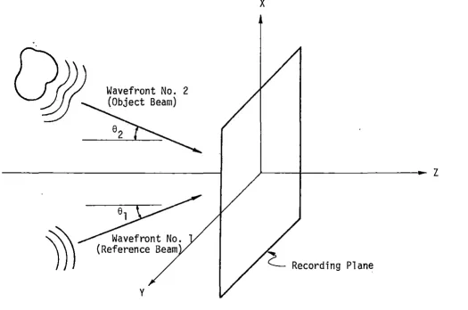
The key mechanism in recording an optical hologram is interference, Figure l. In recording a hologram, the amplitude and phase information are converted into intensity variations using the interference phenomenon l:ietween two interacting sources of light. The two wavefronts in Figure

l interact .an a detecting surface called recording plane. Wavefront No. 2 is the object source or beam and wavefronts are split off from one main source because the reference and the object beams must be mutually coherent. To produce a hologram, the object beam which has become modu-lated when illuminating the surface to be holographed is allowed to interact with the unmodulated reference beam to form the interference pattern. Interference is either constructive or destructive depending

on the path length from a point on the object to the recording plane.

Wavefront No. 2 (Object Beam)

Wavefront No. (Reference Beam

y

z

Recording Plane

with the light from the object to map the relative amplitude and phase of each point on the object into an intensity function on the two-dimensional recording surface (3, 6).

Mathematical analysis of recording process

The mathematical model of holographic recording used here is that given by Hildebrand and Brenden (5). This model is a general

mathematical model which can be applied to both optical and acoustical holography. In this model, real notation is used and the time-dependent terms are retained. This is done because long wavelengths of radiation

were consi.dered where it is not' as obvious that the time dependence can be

ignored as is apparent with optical radiation.

Consider two beams of radiation intersecting on a detecting plane, Figure l . These two beams are mutually coherent. Thus, phase

differences between any two equal length segments of the beam are equal and independent of time. The instantaneous amplitude of beam l at point (x, y) on the recording surface can be described as

s1 (x, y) = a1 (x, y) cos [wt + <P_{1 (x, y)]} ( l )

while the instantaneous amplitude from beam 2 can be described as

(2)

where .a(x, y) is the amplitude of the wave, tj>(x, y) is the phase of the

wave and w is the angular frequency of the wave in radians/sec. The

= a1(x, y) cos [wt+ cp_{1(x, y)J + a2(x, y) cos}

[wt + cp₂ ( x , Y)] • (3)

. In optical radiation, the radian frequency_ is so great that no detector exists that can detect the oscillation (5). Hence, the best thing to do is to measure intensity. The signal that is recorded is some function of intensity

I(x, y) =< [s(x, y)J 2>t (4)

where< >t denotes an average over many cycles of radiation. Now if Equation 3 is substituted into Equation 4, the result is

where

2 2

s1 = 1/2 a1 (x, y)<{l +cos 2 [wt+ cp_{1(x, y)}>t}

~(x, y)J >t

easily because an oscillating function such as cos wt averages to zero over many cycles. Therefore, Equation 5 reduces to

2 2

I(x, y)

=

As seen in the equation above, we have succeeded in preserving the phase terms of both wavefronts.

Reconstruction

(6)

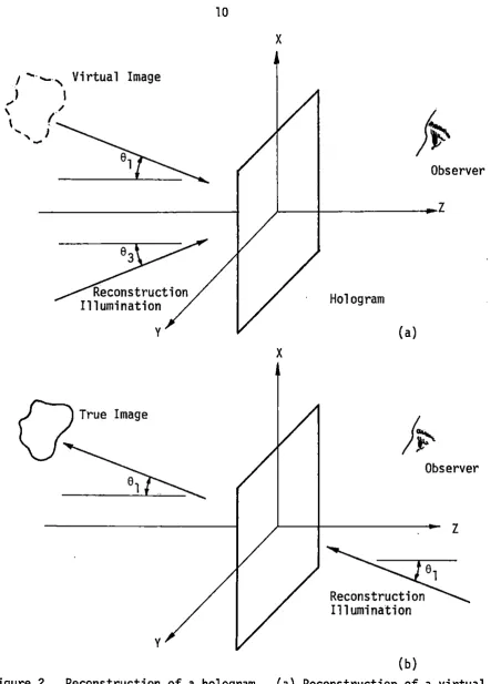
The next step in creating a three dimensional image or hologram is to reconstruct the phase and amplitude information. This is done by using the diffraction phenomenon. The recorded hologram is illuminated by a coherent wave, Figure 2. The recorded fringes on the hologram act as diffraction gratings and cause the coherent incident beam to be

diffracted. The diffraction in turn recreates a wavefront which carries the phase and amplitude information of the original wavefront. Producing a virtual image, Figure 2a, or a true image, Figure 2b, of the object, depends on the direction which the coherent reconstruction wave is illuminating the hologram.

Mathematical analysis of reconstruction process

As noted, the information recorded on a sensitive surface can be reconstructed by the process of diffraction. Here, a general mathematical model of the process as described by Hildebrand and Brenden (5) is

I ... , Virtual Image

I I

--

' I

'-,_;~

Reconstruction Il 1 umi nation

y

y

x

1~

Observer

Hologram

(a)

!~

Reconstruction Illumination

(b)

Observer

z

(7)

Consider a photographic plate which is exposed to the intensity in Equation 6. After development, the plate has a transmittance

proportional to the intensity. Hence, when wave s3 passes through the plate it is modified by this transmittance as

K 2 2

KI(x, y)s3(x, y)

=

2

[wt+ ¢_{3(x, y)J + K/4 a1(x, y)a2(x, y)}

a3(x, y) {cos [wt+ ¢_{1(x, y) -} ¢_{2(x, y)}

+ ¢_{3(x, y) +cos [wt -} ¢_{1(x, y) +} ¢_{2(x, y)}

where K is a constant related to the sensitivity of the photoplate. Let us consider the terms one by one. The first term is actually the

(8)

reconstruction wave which has been modified in amplitude. To demonstrate that either one of the waves, s1 or s2 of Equations l and 2 respectively, can be reconstructed by diffracting the other beam through the hologram, some assumptions should be made. Assuming that s3 is a replica of s2, the second term in Equation 8 becomes

K 2

4

which represents the original wave, s1, with a modified amplitude. With the same assumption, the third term of Equation 8 becomes

(10)

This is an extraneous.tenn which tends to mask the light from the desired wave.

Several other options are available. For instance, consider that s3 is the exact duplicate of s1 ; therefore, the third tenn of Equation 8 becomes

( 11)

The second tenn becomes

It can be seen here that s2 is reconstructed. Additionally, by using the conjugate of one of the interfering beams as the diffracting beam, the conjugate of the other can be reconstructed.

Acoustical Imaging Using Liquid-Surface Levitation

The basic principles described above can also be applied to

of the object and reference beams. In acoustical imaging, the two beams can thus be from two different sources-which are driven from the same generator. The most frequently used methods in generating sounds

involve magnetostrictive or piezoelectric devices. The magnetostrictive devices are capable of generating high acoustic powers, but are limited to frequencies below 100 KHz. On the other hand, the piezoelectric converters are capable of producing frequencies in the vicinity of 100 MHz in liquids (7). In addition, they can operate at the lowest ultra-sonic power level of any detector available.

Recording_ and reconstruction

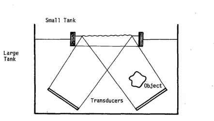
Consider the situation of a liquid-air interface as illustrated in Figure 3. The two transducers A and B are submerged in a liquid. A stationary sound wave impinging on a liquid-air interface exerts static pressure on this surface. This radiation pressure is proportional to the intensity of the impinging wave.

Transducers A and B are driven by the same generator and therefore produce mutually coherent ultrasonic waves. Let us consider that

transducer A insonifies the object. Therefore, the beam from trans-ducer A will be modulated by the object and the waves behind the object carry the ultrasonic information of the object and thus are called the

,

object wave. Waves from transducer B will not be modulated and.hence provide the reference wave. The two beams interfere in the region of. overlap on the surface of the liquid.

~

~

a

Transducers

Figure 3. Formation of static ripples as an acoustic hologram at the liquid-air interface. Transducer A acts as the object transducer and transducer B as the reference

Large Tank

Small tank

abject

Transducers

interference pattern: the acoustic radiation pressure, the surface tension, and gravity ( l). These three forces will interact and as the result of their interaction the surface of the liquid wi 11 deform. The deformation includes an overall elevation of the surface and in

addition, the production of surface ripples. The surface deformation is proportional to the acoustic intensity. Therefore, the

liquid-surface acts as an intensity-sensitive detector; Or, in other words, a hologram can be produced on the surface of the liquid.

Since the liquid surface carries the acoustic information due to acoustical interference, a photograph can be taken from the stationary

ripples on the liquid surface and it becomes an acoustic hologram (9.).

The recording step of taking a photograph is not necessa•ry for creating an acoustic image. The acoustic hologram information is already available

at the surface of the liquid. Therefore, by illuminating the liquid surface witli a coherent light source, the ultrasonic object information can be reconstructed directly and immediately.

Therefore, the reconstruction of the image can be done either

will undergo different optical path lengths according to the surface configuration. This means that the rippled surface can directly

diffract the incident laser light just like a hologram. Therefore, the result of this diffracted light is a product of hologram reconstruction which is a replica of the object wave. Because the recording step is obviated, the optical replica of sound information can be made without delay, thus it allows real-time formation of acoustic images.

The system used in this experiment has several serious problems which have to be considered and solved.

The sound wave has basically three effects on the free liquid-surface on which it impinges (7): l) a uniform levitation, 2) defor-mation superimposed on the levitation (the main holographic infordefor-mation), and 3) small perturbations of the deformed surface. As described

later in Chapter III, it is desirable to increase the height of the vertical deformation or ripples and reduce the overall levitation. In the next chapter, it will be shown that the ripple height and the overall levitation are inversely proportional to surface tension of the liquid y, and the density of the liquid p. Thus, it is preferred to use liquids of low surface tension and high density.

is much reduced when the reconstruction is performed at a short time ihterval around the instant when the ripple formation is maximized if the sound is pulsed at rates ranging from one hundred to several hundred times per second. Considerable gain in effective surface flatness and surface stability can be gained using this technique.

Because of the dynamic response of the surface, the laser beam has to be pulsed in synchronism with the acoustic pulses. The pulse is

usually flashed on shortly (300 µsec) after the acoustic pulse is off for 5-50 µsec at the time when the surface hologram is fully developed.

A sound beam in absorbing liquids such as water sets up streaming and turbulence at the surface which impair the image and affect the reconstruction. Pulsing the sound is one way to reduce the amount of streaming.

Another arrangement can be used to stabilize the effect of

streaming and turbulence ( l, 2). In· Figure 4, two tanks containing liquid are shown - a large tank and a small imaging tank. The small tank lies on top of the large tank and is separated from the large tank by a membrane. This membrane is transparent to the sound but isolates the streaming and unwanted fluid motion in the lower tank from the

Geometry and Mathematical Analysis

the configuration of the insonified liquid surface is shown in Figure 5.

The following is the analytical treatment of this technique by

Smith and Brenden (as cited in 8, Chapter 1). Assume that 28 is the ob-ject and the reference sound waves incident on the liquid surface.

The whole surface is levitated by h_{0 •} The distance between the

ripples is d, and the height of ripples is, h. The coherent light is

incident at an angle a for real-time reconstruction and is reflected at

the same angle. The reconstructed waves are diffracted at an angle (a +

<Sa). Assume that the sound wave has a frequency off and a wavelength

of A, the light wavelength is A. and the intensity is I, then for the ideal

geometry

(sin a)/A.

=

This equation implies that regardless of e, a is very small and the

technique can be safely considered as on-axis holography. The distance between ripples is then

d

=

This equation is dependent on the sound wavelength while the ripple height h,

is a function of the sound intensity, its velocity of propagation c,

frequency f, the angle 8, and the surface tension y. To obtain more

efficient light diffraction, it is desirable to increase the height of the ripples. Therefore, it is preferred to use liquids of low surface tension. On the other hand, overall levitation of the liquid

h₀

=

should be minimized, by using liquids of high density p. To have a large separation between the optically reconstructed images, i.e., to have a

large

oa,

e

wave should be maximized. However, the increase of f and 8, reduces the

~ip~les' height h.

The angle ca is given by

ca= (A.sin 8)/(J\cos a).

A practical compromise between having a large h, Equation 15, and a large a, Equation 17, has led to the useful criterion

f(MHz)· sine " .233.

Computing the Distance Between Ripples

( 17)

( l8)

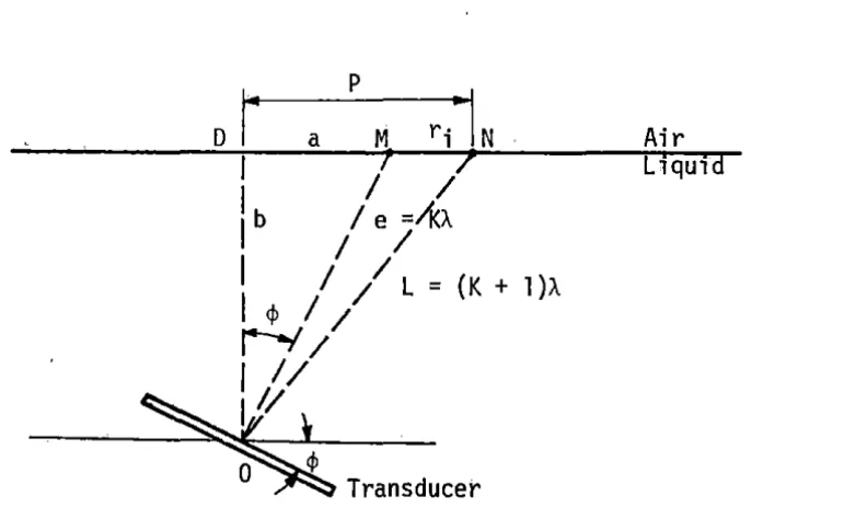
Figure 6 illustrates the position of the transducer relative to the surface of the water.

Light

(Wavelength t.)

Reference Beam

e_.._.e

+

oct

Ultrasound Wave 1 ength A Velocity c

Intensity I

Air Liquid

(Density p)

Object Beam

Figure 5. Configuration of the insonified liquid-surface. The object

and the reference beams are incident at the same angle

e

p

a Air

Liquid

wavelength of the sound. Therefore, e and L can be introduced as

e = kA ( 19)

and

L=(K+l)A (20)

then

L-e =A ( 21)

which can be generalized as

L-e

=

Computing the distance between the ripples in terms of the distance of

the transducer from the water surface, b, and the angle of incidence cf>

results in

where

and

Therefore,

e

=

p=a+r. ₁

a = b tan cf> •

for i

=

L-e = [p2 + b2] 1/2 - c~scj> = mA

[p2 + b2] 1/2 = _b_. + mA

and

= [(-b-+ mA)2 _ b2]1/2

P cos<!>

r.

=

i cos<!>

and n

=

Experimental Equipment

(30)

( 31)

The system used in this experiment consisted of a rectangular water~

tank, two ultrasonic transducers, a coherent light source, and a radio frequency generator. Figure 7 illustrates the system used.

The water tank was made out of plastic. The tank dimensions were 29 x

24 cm at the bottom and 33 x 28 cm at the top.

The tank was filled with water to a depth of 10 cm. This depth was chosen because, after many experiments with different depths, it was found out that at this depth the fringes were more visible.

The system was arranged on the laboratory floor to isolate the liquid from the external vibrations. The slightest vibration in any of the equipment caused the image to vibrate and produced a blurry and un-stable image. When vibrations are transmitted directly to the water tank the image swings widely in the space. Therefore, it was essential to have a very, steady and stable geometry to avoid any unwanted exterrial interference.

.-

_..

_.

. ~ .

.

·.

_.

_.

... • ' : : •, I •

. "

....

.

Transducers

Figure 7. Schematic diagram of the set-up

Water

Tank Oscilloscope

0

Generator

N

one millimeter thick and were coated with a silver alloy to provide con-duction for electric current. They operated at resonance frequency of about 2.2 MHz.

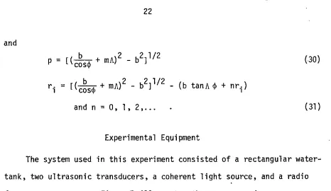
Since the transducers were not equipped to be immersed in water, mounting devices were fabricated. Figure 8 shows the mounting devices and the location of the transducers. Two 2.54 x 2.54 cm stainless steel blocks were built. A well with a diameter of 2.54 cm and a depth .of ' about one millimeter (the dimensions of the transducer) was cut in the middle of each block. The thickness of the block directly underneath the transducer was chosen to be an integral number of half wavelengths of the sound in the steel to eliminate the destructive waves bouncing back from the bottom of the blocks.

For a frequency of 2.2 MHz, and the velocity of the sound in steel of 5790 m/sec we have

A

=

=

f 2.2 MHz

The thickness of block underneath the well was 13.2 mm which is

(32)

approximately 5 wavelengths. Of course, to obtain the optimum resonance frequency, the frequencies of the transducers still needed some adjusting th.rough the frequency generator.

Two screw holes were drilled, one on each side of the well on each block, to provide electrical connection sites to transducers.

5.8

cm

(a)

4.9

cm

5 cm

.:::::================01

I

I

I I I

I / I I I //

I /

I I ,,,,,. ,,,.

( _{... I} I _{,,.. ,,.} /

... .J,.,,.

(c)

IT

IT

~~4

r

~g

fL5cm_J

( b)

Metal Block

Figure 8. Schematic diagrams of the mounting devices. (a) top view of the stainless blocks used to hold the transducers. (b) side view of the block, (c) the stand used to hold the metal blocks

N

was avatlable. Therefore, it was not convenient to reach the other side

of the transducer through the block. The second reason was that soldering wires to ceramic transducers had to be done very rapidly to avoid any damage to the transducers due to too much heat. Also, the wires should be thin and flexible and soldered with the least amount of solder possible. Since, in this experiment, there was considerable handling and movement of the transducers and wires, the connections or wires would be likely to fail. Therefore, it was decided to use a pressure spring technique instead. This was done by simply holding down the transducer by a piece of metal and creating enough pressure through the. metal on the surface of the transducer to form the electrical connection. In this experiment, a small piece of brass was screwed

down on the block on one side of the transducer at a screw hole which was provided for this purpose, Figure Ba. The other side of the brass was barely touching the transducer and exerted enough pressure on the transducer to have a proper electrical connection. To prevent the brass from connect1ng to the metal block and shorting the circuit, plastic screws and washers were used. To provide an electrical ground, a wire was attached to the other screw hole on the block on the side opposite the brass spring.

two screw holes on the sides of the blocks, Figure Sb. They were used to hold the blocks in the slit. At the same time, the blocks could slide freely back and forth along the slit. This feature gave the freedom of positioning the transducers at different angles with the water surface and also at various dis.tances from one another.

The transducers were driven by a IEC F34 frequency generator ( IEC, Anaheim, CA.) which provides a frequency up to 3 MHz and an output voltage of 10 volts peak to peak.

The. connections between the oscillator and the transducers were provided through a switch system which allowed one to operate the

trans-"

ducers individually or simultaneously.

An oscilloscope monitored the output voltage of the transducers. A Helium-Neon laser (Spectra-Physics, Inc., Mt. View, CA.)

was used as the coherent light source at A 0

=

was used to appropriately position the laser for optical illumination of the water surface. The angle of illumination. in this experiment was about 70° from the horizontal.

Technique and Targets

As indicated earlier, the technique used in this experiment to visualize the diffraction pattern of the ultrasonic waves was to use liquid-surface as the recording medium.

the dust in the air which floated on the water surface, produced

secondary fringes around themselves and confused the pattern due to the sound waves. Also, the larger particles on the surface created shadows which blocked parts of the ultrasonic pattern. Thus, it was important to hav,e a pure liquid and a clean surface.

A continuous sound wave having a frequency in the range of 2.16 MHz to 2.45 MHz was used. The exact frequency depended on the target, as will be discussed in greater detail in the next chapter.

Two different sets of experiments were done. The first set was done with only a single transducer, and the second with both transducers. These sets were also divided in two other subsets, one without any targets and the other with various targets. In each experiment, . tile transducers were placed at various positions and angles with re,spect to the surface of water and also with respect to each other (two transducers). In

experiments with a single transducer, the sound field pattern produced by the object wave sound wavefronts were observed. An interference pattern due to interfering beams of two transducers was observed in the second set of experiments. A number of different target materials was used

aluminum, plexiglass, and animal tissue in the form of the hind leg of .a rat. The sound field patterns were also observed with these targets.

using different shutter speeds ranging from 1000 seconds to several seconds. The most useful results were observed when the shutter speed

l l

was between 125 to 60 second. The photographs were taken in complete darkness, except for the laser beam.

The camera was attached to a tripod and a cable release was used to ensure the steadiness of the images.

The oscillator was set at 10 volt peak to peak continuous sinewave. Two 0.001 µF capacitors were put between the oscillator and the

trans-ducers to prevent any DC current from passing through the transtrans-ducers, Figure 9.

As mentioned earlier, the laser was set at an angle of about 70.~ to

horizontal. A spatial filter, an aperture, and a lens were placed in the laser beam. The spatial filter was used to enlarge the beam and also improve its quality. The aperture eliminated the peripheral beam fringes and the lens was used to produce a collimated beam. This beam

illuminated the surface of the water and had a width of about 2.8 cm. As dtscussed earlier, the experiments were done in two parts. In the first part, a single transducer was used and in the second part the same experiments were repeated using two transducers. In the next two

sections, the experiments are described step-by-step without discussing the results. The results will be discussed in the next chapter.

One transducer

follows~

a) The transducer without any target, b) The transducer with a target.

Each group can also be divided to smaller groups as: 1) The transducer vertical

2) The transducer tilted

at an angle ¢

=

at an angle ¢ = 15°.

The targets used in these experiments were aluminum, plexiglass and the hind leg of a rat.

Two transducers

The experiments, with two transducers ca~ be grouped as follows:

a) Transducers without a target b) Transducers with a target.

In these experiments, both transducers are tilted and they can be divided as:

1) Transducers facing each other

- at an angle ¢

=

- at an angle¢'

=

2) Transducers at right angles to one another.

The targets used were the same as in the experiments with one

transducer. Each target was placed in front of only one of the trans~

ducers. This transducer was defined to provide the object beam while the other transducer provided the reference beam. The changes in surface pattern (if any) were observed and recorded.

Generator

Capacitors

.----1

1---fl<Doh

.,...

As mentioned in the previous chapter, the results of the experiments were documented on photographic film. In· this chapter, these photographs will be presented and discussed.

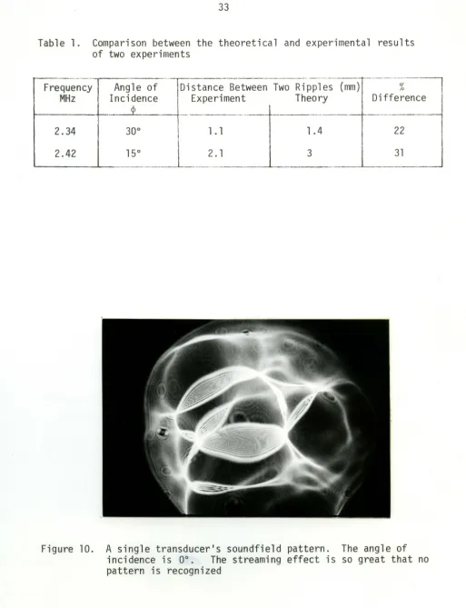
An attempt to observe the sound field pattern of a single transducer

sending the sound waves perpendicular to the water surface (~

=

resulted in the pattern shown in Figure 10. The operational parameters

were as follows:

f

=

v

=

d

=

There is no obvious uniform pattern as the result of the sound wave-front. Most of this nonuniform pattern is due to the streaming effect. Other oscillation frequencies were tried with no apparent ·change toward

improving the pattern. It is obvious that at 0° angle the effects of

streaming and overall elevation are so great, at least under the

conditions of this experiment, that the ultrasonic wavefront pattern is impossible to observe.

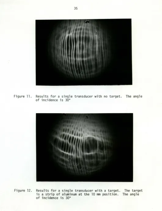
Figure 11 is a photograph taken from the acoustical pattern

produced with a ~ingle tilted transducer. There was no target present

in ·this experiment. The operationa 1 parameters were as follows:

f = 2. 34 MHz

v

=

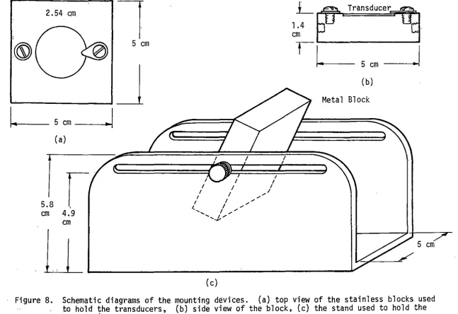
Table l. Comparison between the theoretical and experimental results of two experiments

---·--· ·--··-·-~ -

-Frequency Angle of Distance Between Two Ripples (mm) o/ ₁₀

MHz Incidence Experiment Theory Difference

cp

-~·-· ---· -~ ·-

--2.34 30° l. l l.4 22

2.42 l 5°

L

-- - --- -- -

The camera exposure time was 1/125 sec.

It can be seen in Figure 11 that the pattern is relatively uniform.

The light and dark lines represent the ripple pattern produced by the ultrasonic wavefront incident on the water surface. The bright lines result from reflection of the laser beam from the ripples. The lines are more clearly visible in the center and become less distinct as the perimeter of the area is approached. Also, the distance between the bands is greater in the center than between bands approaching the left

and right edges of the circle. From :~quation 31 in Chapter III, the

distance between the ripples ·will be calculated form

=

b

=

<P

=

Then from Equations 26 and 23

a

=

=

=

b 42

e

=

=

=

(33) (34)

(35)

(36)

and the wavelength of the sound for a frequency of 2.2 MHz and velocity of 1460 m/sec in water will be

A = 1460 m/sec :: 6

2 • 34 MHZ - ' mm ' (37)

Substituting these values in Equation 31 results in

r1

=

.6)

1

=

and

Figure 11.

Figure 12.

Results for a single transducer with no target. of incidence is 30°

Results for a single transducer with a target. is a strip of aluminum at the 10 l11Tl position.

of incidence is 30°

The angle

Figure 13. Results for a single transducer with a target. The target is at the 15 mm position. The angle of incidence is 30°

These results clearly show the effect of moving further from the center to the left and. right edges of figure.

Table 1 compares the experimental and theoretical results of two of these experiments.

The distortion in the middle of the pattern, the bright circles crossing the diffraction pattern of the ultrasonic wavefront, is due to the overall elevation of the water and the streaming effects. The

generally c;i rcul ar secondary patterns were produced by the dust pa rti cl es floating on the surface of the water.

Figures 12, 13, arid l 4 are the photographs of the same pattern with .an aluminum strip as the target. The aluminum was about 1.3 cm wide and about 1 millimeter thick. The target was attached to a micromanipulator in order to allow movement over small distances with least disturbance of the water. The distance between the target and transducer was about 1.9 cm. The target was initially positioned at the edge of the trans-ducer (not covering any part of the transtrans-ducer) and moved in increments of 5 mtll imeters across the transducer. Figure 15 i 11 ustrates how the target was moved over a range of 25 mm to obtain various results. In each position, the pattern change was observed and recorded. Figure 12

Target

Transducer

__ ,... O mm _{5 mm} _ _ .,.. lQ mm

_ ____,~ 15 mm _ __,.,..20 mm _ __,.,..25 mm

Figure 15. Different positions of the aluminum target with respect

Figure 12 has the most complicated and distorted pattern. It .seems

that the target also produces some secondary patterns in the area blocked by the target. These patterns appear to cross the initial pattern. As the target moves toward the other side of the transducer, Figure 14, the regular pattern emerges again.

The next two Figures, 16 and 17, compare the sound field patterns without and with a target. The target in this experiment is again the aluminum stri.p but the angle of inci:dence is smaller. The operational conditions for this experiment were as follows:

f

=

V

= •

d

=

¢

=

These figures distinctly show that the distances between the bands are greater as compared to the previous experiment. The results of compari-son between theory and experiment are shown in Table l. Comparing

Figures 11 and 16, it can be seen that in Figure 11 where ¢

=

ripples are much closer together than are the ripples in Figure 16 with

¢

=

The effects of streaming.and overall elevation are more prominent in the experiment with a smaller angle of incidence. Therefore, it can be deduced that these disturbances are greatest for ultrasonic beams

perpendicular to the fluid surface.

Figure 16. Results for a single transducer with no target. The angle of incidence is 15°. The distance between the bands is much greater as compared to Figure 11

front of the transducer at a distance of approximately 1.9 cm. The target was placed at the 5 mm position, Figure 15. As can be seen here,

Figure 16, the streaming effect is reduced and the "crosswise" patterns

are beginning to form.

Figures 19 and 20 show the changes in ultrasonic patterns due to

a strip of ~exiglass used as the target. The target was a piece of

Plexiglass .6 cm thick and 1.2 cm wide. The approximate distance between

the target and transducer was about 3.3 cm. The experimental conditions

were as fo 11 ows :

f = 2.37 MHz

v

=

d = 33. 7 cm

cp

=

The experiment was conducted with the target in two different

positions: 1) the target covering approximately half of the transducer, and 2) the target covering the middle part of the transducer, as shown in Figure 21.

Figures 19 and 20 show the changes in the pattern of the ultrasonic

wavefront with the target in positions (a) and (b) of Figure 21, respectively.

Figure 18. Results for a single transducer with no target. The angle of incidence is 30°

Figure 20. Results for a single transducer with plexiglass target covering half of the transducer

l .2cm

Target

Transducer

(a) (b)

appears near the middle of the figure. This area seems to be a direct result of the overall elevation of the water. On the outer edges of the illuminated area, most visible at the bottom of the figure on the right side, there is a slight curving of the bands. This distortion is probably due to the brass spring used as the electrical connection for the transducer.

In Figure 19, the pattern in the area covered by the target (the bottom half of the figure) seems to be more uniform. It seems that the target does not block or alter the sonic wavefront from forming the

ripples on the water surface. It probably only modifies the amplitude of intensity. This, in turn, causes the streaming effect to be reduced to some extent. The very bright line across the middle of the figure

indicates the edge of the target.

Figure 20 shows the pattern with the same target but in a different position, Figure 2lb. Both edges of the target are clearly visible here.

Figures 22, 23 and 24, taken from the ultrasonic wavefronts,

represent experiments where the target was the same as in the previous experiment, but a smaller angle of incidence was used. There was no target used in the experiment represented in Figure 22. The operational parameters were as follows:

f=2.4MHz

v

=

d

=

The distance oetween the target and transducer was about 2.7 cm. The obvious increase between the bands due to a smaller angle. can be observed again.

In Figures 23 and 24, the effect of placing a target in front of

the transducer is clearly shown. In Figure 24, the shape and position

of the target is clearer. It appears that there is less distortion in the pattern where the target is not covering the transducer compared to

Figure 20.

Figures 25 and 26 are the photographs of the ultrasonic wavefronts

without and with a target, respectively. The target in this experiment was mammalian tissue (the hind leg of a rat). For this purpose, ,a rat

weighing about 330 gm was killed by sodium pentobarbital and the leg was

removed. The leg was suspended with two threads and immersed in the water in front of only one transducer. The operational conditions were as follows:

f

=

v = .45 volts

d = 33.4 cm

cf>

=

The part of the leg which was used as the target had a circumference of

about 2.6 cm and was placed at a distance of about 2.3 cm from the

transducer.

Figure 22. Results for a single transducer with no target. The angle of incidence is 15°

Figure 24. Results for a single transducer with plexiglass target covering the middle part of the transducer

Figure 26. Results for a single transducer with mammalian tissue as the target

Figure 28. Results for two transducers with aluminum target at the

15 mm position. The target is in front of only one transducer

can be seen in the background of the lower half of Figure 26. The bright lines interfering with the pattern appear to be a reslJlt of streaming effect and overall elevation which have been spread into this particular shape as a result of placing a target in the path of ultra-sonic beam.

Figures 27, 28 and 29 are the interference patterns of two

trans-ducers. Figure 27 is the interference pattern without any targets.

Figures 28 and 29 are the same pattern except that a target was placed

in front of one of the transducers. The operational parameters were as follows:

f

=

v

=

d

=

$

=

The target used in this experiment was the same piece of aluminum which was used earlier with one transducer. The experimental scheme was exactly the same also. The target was moved in increments of 5 mm each time for a total distance of 25 mm, Figure 15.

The target was placed in only the object beam. The other transducer was acting as the reference beam and was aimed directly toward the water surface.

In Figure 27, the pattern appears to be much more uniform compared to

Figure 28 was made with the target placed in the 15 mm position, Figure 15. The top half of the figure is where the target was placed. It is obvious that not all the ultrasonic energy has reached the water surface. There is a significant change in the bottom half of the pattern which was not covered with the target. The very complicated pattern is obviously due to the presence of the target which interacts with other sources of distortion such as streaming.

Figure 29 is the interference pattern with the target in the 25 mm

position, Figure 15. The pattern is not as complicated as in the

previous figure. It seems that placing the target over the middle part of the transducer has modified the pattern to some extent. I.t appears that moving the edge of the target toward the center of the transducer generates this special effect, Figure 28.

The last set of experiments was done with transducers at right

angles with respect to each other as illustrated in Figure 30. The

operational parameters were as follows:

f = 2.45 MHz

v₁

=

v₂

= .

d

=

$₁

=

$₂

=

Figure 30.

I I

goo

L __ ..___

Metal Blocks

The position of the transducers relative to each other.

Figure 31. Results for two transducers at right angles with no target. The angles of incidence are 60° and 43°

clearly shows the effect of interference of the ultrasonic beams produced by both transducers. The primary bands run diagonaTly from right to left at an angle of 45° to horizontal as would be expected.

Figure 32 is the same pattern with the target in front of the

transducer with the angle of incidence ~

₂

=

CHAPTER V. SUMMARY AND CONCLUSIONS

An attempt was made to visualize the ultrasonic wave pattern via deformation of a liquid surface. The method employed is one of the techniques commonly used to generate acoustical holograms.

The system consisted of a water surface which ,acted as the visualizing

plane and one or more transducers ~1hose output waves impinged upon the

water surface to produce ripples. Coherent light produced by a laser was used to illuminate the water surface.

The experiment was conducted primarily in two parts: 1) using a

single transducer, 2) using two transducers.

The system showed extreme sensitivity to disturbances such as

streaming effect of the water; however, the ultrasonic pattern in all ex-periments was almost completely visible. The results of the experiment with '.two transducers simultaneously showed more uniformity of ripple

pattern and less distortion.

The distances between ripples were measured and compared with theoretical values. "fable l shows the results of this comparison. The experimental results could not be measured very accurately due to dis-tortions and the comparison showed a difference of about 30% between the experimental and theoretical results.

Tests were done with different targets in front of the transducers. The technique was shown to be successful in visualizing the ultrasonic wavefront pattern and also an effective way to visualize the ultrasonic

1. Ahmed Mahfuz, K. Y. Wang., and A. F. Metherell. 1979. Holography and Its Application to Acoustic Imaging. Proc. of the IEEE, 67 (4): 466-483.

2. Aldridge, E. E. 1971. Acoustical Holography. Merrow Publishing Co. , Ltd. , Watford, Herts, Engl and.

3. Goodman, J. W. 1968. Introduction to Fourier Optics. McGraw-Hi 11, Inc., San Francisco.

4. Green, P. S., Ed. 1973. Acoustical Holography. Vol. 5. Plenum Press, New York.

5. Hildebrand, B. P., and B. B. Brenden. 1972. An Introduction to Acoustical Holography. Plenum Press, New York.

6. Lehmann, Matt. 1970. Holography, Technique and Practice. The Focal Press, New York.

7. Methere 11 , A. F. , H. M. E 1-Sum, and Lewis Larmore, Eds. 1969. Acoustical Holography. Vol. 1. Plenum Press, New York. 8. Metherell, A. F., and Lewis Larmore, Eds. 1970. Acousti.cal

Holography. Vol. 2. Plenum Press, New York.

9. Mueller, R. K., and N. K. Sheridon. 1966. Sound Holograms and Optical Reconstruction. Appl. Phys. Lett., 9:328.