City, University of London Institutional Repository
Citation:
Wood, J. and Dykes, J. (2008). Spatially Ordered Treemaps. IEEE Transactions
on Visualization and Computer Graphics, 14(6), pp. 1348-1355. doi:
10.1109/TVCG.2008.165
This is the unspecified version of the paper.
This version of the publication may differ from the final published
version.
Permanent repository link:
http://openaccess.city.ac.uk/536/
Link to published version:
http://dx.doi.org/10.1109/TVCG.2008.165
Copyright and reuse: City Research Online aims to make research
outputs of City, University of London available to a wider audience.
Copyright and Moral Rights remain with the author(s) and/or copyright
holders. URLs from City Research Online may be freely distributed and
linked to.
Spatially Ordered Treemaps
Jo Wood,Member, IEEE, and Jason Dykes
Abstract—Existing treemap layout algorithms suffer to some extent from poor or inconsistent mappings between data order and visual ordering in their representation, reducing their cognitive plausibility. While attempts have been made to quantify this mismatch, and algorithms proposed to minimize inconsistency, solutions provided tend to concentrate on one-dimensional ordering. We propose
extensions to the existingsquarifiedlayout algorithm that exploit the two-dimensional arrangement of treemap nodes more effectively.
Our proposedspatial squarified layout algorithm provides a more consistent arrangement of nodes while maintaining low aspect
ratios. It is suitable for the arrangement of data with a geographic component and can be used to create tessellated cartograms for geovisualization. Locational consistency is measured and visualized and a number of layout algorithms are compared. CIELab color space and displacement vector overlays are used to assess and emphasize the spatial layout of treemap nodes. A case study involving locations of tagged photographs in the Flickr database is described.
Index Terms—Geovisualization, treemaps, cartograms, CIELab, geographic information, tree structures.
1 INTRODUCTION
The use of treemaps, first proposed by Shneiderman [21], to represent hierarchical data has received wide attention in the information visu-alization community [22]. Their compact use of graphical space, re-duced graphical complexity, relative ease of computation [24] as well as some high profile examples (e.g. [25]) have all contributed to their popularity. Yet they have also received criticism for their lack of cog-nitive plausibility [9], poorly perceived aesthetic qualities [6] and poor task-driven performance [1, 6].
In this paper we address some of the weaknesses of existing treemap layout algorithms and presentation conventions by focussing on node placement. Our aim is to use location (a ratio-scale property) to rep-resent relationships within hierarchical levels to produce ‘richer and less opaque’ representations and address concerns relating to the cog-nitive plausibility of treemaps [24]. In doing so, we produce treemaps that may be used more effectively for answering queries that involve identifying relationships and trends within datasets.
2 ORDEREDLAYOUTS
Nodes in a treemap represent individual data items in some dataset and their size, color and text label can be used to represent attributes of the data item. The topological relationship with higher level containing nodes is used to show the item’s position in the hierarchy. However in most treemaps, the node’s position does not precisely represent any charactersitic of the data. This is a potential waste of the information carrying capacity of the treemap and can also reduce the clarity of the representation by violating the distance-similarity metaphor [10] (the same data can be represented in arbitrarily different looking treemaps depending on the ordering of nodes).
The problem is illustrated in Figure 1. Here, 256 nodes of unit size are arranged using thesquarifiedlayout [5] that attempts to min-imise aspect ratios. Nodes are approximately ordered from top-left to bottom-right. To search for a node early in the sequence (dark green), we would need to look somewhere towards the top or left. However the relationship between node order and distance from the top-left is not a simple one in this layout (Figure 1b). In this example nodes 0-15 show a consistent linear relationship between order and distance. However the next node in sequence, node 16 is as close to the corner as node 1. These large jumps in distance-node order relationship make locating a given node more difficult. Spatial discontinuities also make it difficult
• Jo Wood ([email protected]) and Jason Dykes ([email protected]) are
based at the giCentre, School of Informatics, City University London.
Manuscript received 31 March 2008; accepted 1 August 2008; posted online 19 October 2008; mailed on 13 October 2008.
For information on obtaining reprints of this article, please send e-mailto:[email protected].
to infer node order directly from location without significant cognitive effort and so impede efforts to identify relationships and trends.
Bedersonet al[2] attempted to address an aspect of this problem by considering various ordered layout algorthims where “items that are next to each other in the input to the algorithm are adjacent in the
treemap” [2, p.836]. They recognized that the linear ordering of nodes
could be used to emphasize trends in a dataset as well as aid naviga-tion through it. They proposed a metric,readability, that attempted to quantify the ease with which an ordered sequence could be followed in a treemap. This was measured by counting the number of abrupt angular changes (of more than 6 degrees) required when moving in sequence though a set of ordered sibling nodes. While this measure identifies angular change, it does not take into account the distance of separation between adjacent nodes, nor the consistency with which position relates to order.
This is illustrated in Figure 2, which shows four layouts of 16 or-dered unit-sized nodes and their respective readability scores. No an-gular change is required to proceed from node 1 to node 16 in the slice and dice layout, so it receives a maximum readability score of 1. The
strip layout[2] only requires a change in direction when proceeding
from one row to the next, so receives the second highest readability score. Thesquarifed[5] layout requires angular changes that increase in frequency towards the end of the node list. The fourth layout, here termedordered squarifiedrequires some form of angular change be-tween almost all nodes, so receives the lowest readability score. How-ever there is a consistency in this fourth layout not possessed by the strip or squarified layouts that shows a gradual decrease in node rank from top-left to bottom-right.
Tu and Shen [28], attempted to give greater importance to two-dimensional position by overlaying some known image (they used a map of the United States) on the treemap. This image was then dis-torted according to changes in treemap node size. They argued that knowledge of how and where the image has been distorted can be used to assess node change visually. However, this technique pro-vides a rather loose and arbitrary coupling between node location and distorted image.
The differences in approach to layout strategies is in part a func-tion of the fact that two-dimensional space is being used to represent a one-dimensional sequence of data items (such as time series, alpha-betical ordering or size ordering). This is a specific case of a more general problem of representing one-dimensional sequences of data in two-dimensional graphical space [15]. Existing layout algorithms can tolerate this mis-match between data dimension and representation di-mension if the queries they attempt to facilitate are of the form “where
is node x?”, but only then if there is some form of secondary ability to
11/03/2008 14:56 Tree map
Page 1 of 1 file:///Users/jwo/java/treeMaps/data/squarified256.svg
0 1 2 3 4 5 6 7 8 9 10 11 12 13 14 15
16 17 18 19 20 21 22 23 24 25 26 27 28 29 30
31 32 33 34 35 36 37 38 39 40 41 42 43 44 45
46 47 48 49 50 51 52 53 54 55 56 57 58 59
60 61 62 63 64 65 66 67 68 69 70 71 72 73
74 75 76 77 78 79 80 81 82 83 84 85 86
87 88 89 90 91 92 93 94 95 96 97 98 99
100 101 102 103 104 105 106 107 108 109 110 111
112 113 114 115 116 117 118 119 120 121 122 123
124 125 126 127 128 129 130 131 132 133 134
135 136 137 138 139 140 141 142 143 144 145
146 147 148 149 150 151 152 153 154 155
156 157 158 159 160 161 162 163 164 165
166 167 168 169 170 171 172 173 174
175 176 177 178 179 180 181 182 183
184 185 186 187 188 189 190 191
192 193 194 195 196 197 198 199
200 201 202 203 204 205 206
207 208 209 210 211 212 213
214 215 216 217 218 219
220 221 222 223 224 225
226
227
228
229
230
231 232 233 234 235
236
237
238
239 240 241 242 243
244
245
246 247 248 249
250
251 252 253
254 255
R2 = 0.5428
0 100 200 300 400 500 600 700 800 900
0 16 32 48 64 80 96112128144160176192208224240256
Node order
[image:3.612.49.294.52.171.2]Distance from origin
Fig. 1. Squarifiedlayout of 256 ordered nodes of unit size colored by
order. While there are sequences of graphical order following node or-der, there are also large jumps. Relationship between node order and distance from top-left (the origin) itself varies with distance from origin.
11/03/2008 14:31 Tree map
Page 1 of 1 file:///Users/jwo/java/treeMaps/data/sliceAndDice16.svg
1 2 3 4 5 6 7 8 9 10 11 12 13 14 15 16
12/03/2008 16:09 Tree map
Page 1 of 1 file:///Users/jwo/java/treeMaps/data/strip16.svg
1 2 3 4
5 6 7 8
9 10 11 12
13 14 15 16
12/03/2008 17:15 Tree map
Page 1 of 1 file:///Users/jwo/java/treeMaps/data/squarified16.svg
1 2 3 4
5
6
7
8 9 10
11 12 13 14 15 16 12/03/2008 17:16 Tree map
[image:3.612.366.498.145.231.2]Page 1 of 1 file:///Users/jwo/java/treeMaps/data/orderedSquarified16.svg 1 2 3 4 5 6 7 8 9 10 11 12 13 14 15 16
Fig. 2.Slice and dice[21],strip[2],squarified[5] andordered squarified
layouts of 16 ordered nodes of unit size. Thereadabilityscores of the
four layouts are 1.0, 0.625, 0.375 and 0.125 respectively (1 indicates no angular change, 0 indicates every jump between sequential nodes requires an abrupt angular change).
in two-dimensional space. This in turn makes it more difficult to sup-port queries that relate node order to some other variable attached to each node (e.g.“What is the relationship between stock value and
re-cent stock growth” in a treemap that orders and sizes nodes by stock
value and colors them according to change over time [25]).
We therefore propose a new layout algorithm, theordered
squar-ified layout that attempts to order nodes with two-dimensional
con-sistency by relating node order to Euclidean distance from the parent node’s top-left corner (here termed itsorigin). It is based on the
squar-ified layout algorithm of Brulset al[5], but additionally associates a
two-dimensional location with each node. For a sorted setsofn or-dered nodes that must be laid out inside a containing rectangler, each node is given a location according to the algorithmAllocatePosition:
FunctionAllocatePosition(s,r){
float d←sqrt(r.area /n);
boolean isHorizontal←(r.width<r.height); List positions;
for i←0 to<n{
if (isHorizontal){
x←r.x +mod(i∗d,r.width);
y←r.y +f loor(i∗d /r.width)∗d;
}else{
x←r.x +f loor(i∗d /r.height)∗d;
y←r.y +mod(i∗d,r.height);
}
positions.add(x,y);
}
sortByDistance(positions);
for each node ins{
node←positions(i++);
} }
The process of allocating locations that are exactly equally spaced withinryet cover it comprehensively is a non-trivial one, as it is
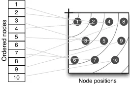
essen-tially a two-dimensional circle packing problem [31]. However, since the algorithm only requires rank order of location sorted by distance from origin, and since nodes of different sizes will only be approxi-mately placed at their nominal location, an approximate tessellation proves adequate by calculating the average distancedbetween nodes. The functionsortByDistance()simply sorts the newly created posi-tions according to their Euclidean distance from the origin(r.x,r.y). An example applied to 10 nodes within a square is shown in Figure 3 .
[image:3.612.49.294.234.296.2]1 2 3 4 5 6 7 8 9 10 10 9 8 7 6 5 4 3 2 1 Ordered nodes Node positions
Fig. 3. Ten nodes located after spacing them within their containing rectangle. Nodes are sorted by distance from the containing rectangle’s origin (the first node is closest).
TheorderedSquarifiedlayout proceeds recursively as in the
origi-nalsquarifiedlayout, but instead of selecting each node in turn from an
ordered list of nodes, it selects the node closest to the current position in the enclosing rectangle. Every time a new node is added, the cur-rent position is movedd units right or down depending on whether nodes are being laid out horizontally or vertically. After each call
to layoutrow() in Bruls’squarifiedalgorithm, AllocatePosition()is
called again to reposition the remaining nodes within the remaining rectangular space.
11/03/2008 14:58 Tree map
Page 1 of 1 file:///Users/jwo/java/treeMaps/data/orderedSquarified256.svg 0 1 2 3 4 5 6 7 8 9 10 11 12 13 14 15 16 17 18 19 20 21 22 23 24 25 26 27 28 29 30 31 32 33 34 35 36 37 38 39 40 41 42 43 44 45 46 47 48 49 50 51 52 53 54 55 56 57 58 59 60 61 62 63 64 65 66 67 68 69 70 71 72 73 74 75 76 77 78 79 80 81 82 83 84 85 86 87 88 89 90 91 92 93 94 95 96 97 98 99 100 101 102 103 104 105 106 107 108 109 110 111 112 113 114 115 116 117 118 119 120 121 122 123 124 125 126 127 128 129 130 131 132 133 134 135 136 137 138 139 140 141 142 143 144 145 146 147 148 149 150 151 152 153 154 155 156 157 158 159 160 161 162 163 164 165 166 167 168 169 170 171 172 173 174 175 176 177 178 179 180 181 182 183 184 185 186 187 188 189 190 191 192 193 194 195 196 197 198 199 200 201 202 203 204 205 206 207 208 209 210 211 212 213 214 215 216 217 218 219 220 221 222 223 224 225 226 227 228 229 230 231 232 233 234 235 236 237 238 239 240 241 242 243 244 245 246 247 248 249 250 251 252 253 254 255
R2 = 0.97
0 100 200 300 400 500 600 700 800 900
0 16 32 48 64 80 96112128144160176192208224240256
Node order
Distance from origin
Fig. 4. OrderedSquarified layout of unit size nodes colored by order.
Euclidean distance from the top-left corner (origin) is approximately lin-early proportional to node order. Variations from linearity are due to forcing a circular distribution into an enclosing rectangle.
The layout applied to nodes of equal size inside a square parent is shown in Figure 4. Summary statistics for four layout algorithms ap-plied to 100 equally sized nodes are shown in Table 1. The metric
distance correlationis simply theR2Pearson Product-Moment
corre-lation coefficient between node order and node distance from the ori-gin. It gives an indication of the order-distance consistency of nodes, although it must be recognized that this relationship is likely to be a non-linear one, so the measure only gives an approximate indication of consistency. Compared with the squarified layout of the same set of nodes (Figure 1), there is greater positional consistency while low aspect ratios are retained. The slice and dice layout has greater consis-tency still, but as has been widely recognized, the poor aspect ratios it produces can make visual comparison difficult [2, 5, 23].
[image:3.612.312.556.389.514.2]31/03/2008 10:36 Tree map
Page 1 of 1 file:///Users/jwo/java/treeMaps/data/squarified100rand.svg
1
2
3
4 5
6
7
8 9
10
11
12
13 14
15
16
17
18 19
20
21
22
23
24
25 26 27 28 29 30
31
32
33
34
35
36 37 38 39 40 41
42
43
44
45
46
47 48 49 50 51
52
53
54
55
56
57 58 59 60 61
62
63
64
65
66
67 68 69 70 71
72
73
74
75
76 77 78 79
80 81
82 83
84 85 86 87
88 89 90
91 92 93 94 95 96 97 98
99 100
31/03/2008 10:39 Tree map
Page 1 of 1 file:///Users/jwo/java/treeMaps/data/orderedSquarified100rand.svg
1
2 3
4 5
6 7
8
9
10 11
12
13 14
15
16 17
18
19
20 21
22
23 24
25
26
27
28
29
30 31
32 33
34
35
36
37
38 39
40 41
42
43 44
45
46
47
48
49
50 51
52 53
54
55 56
57
58
59
60
61
62
63 64
65 66
67
68
69
70
71
72
73 74
75 76
77
78
79 80
81
82 83
84 85
86 87
88 89
90 91
92 93
94 95 96
97 98
99100
Squarified Layout
R2 = 0.84
0 200 400 600 800 1000 1200
0 10 20 30 40 50 60 70 80 90 100
Node order
Distance from origin
Ordered Squarified Layout
R2 = 0.90
0 200 400 600 800 1000 1200
0 10 20 30 40 50 60 70 80 90 100
Node order
[image:4.612.57.565.51.277.2]Distance from origin
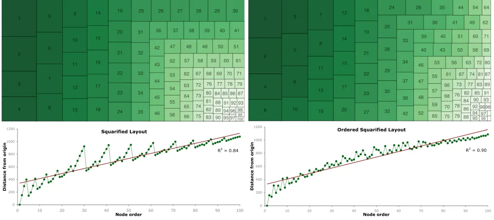
Fig. 5.Squarified(left) andordered squarified(right) layouts of 100 ordered nodes of random sizes. Nodes are colored by order (ordered by size).
[image:4.612.54.301.361.413.2]Tthesquarified layout appears to change approximately half way along its length (node 24) as the aspect ratio in which to fit remaining nodes changes from a horizontal rectangle to being approximately square.
Table 1. Layout statistics for various layouts of 100 equally sized nodes.
Layout Aspect ratio Readability Distance correlation Slice & dice 99.02 1.00 1.00 OrderedSquarified 1.00 0.02 0.97
Squarified 1.00 0.66 0.56
Strip 1.00 0.82 0.57
theordered squarifiedlayout, sets of randomly sized nodes were
cre-ated. Each treemap consisted of 100 nodes each given a random size drawn from a log normal distribution, consistent with the simulations reported in Table II of [2]. Nodes were laid out using thesquarified,
or-deredSquarified,slice and diceandstrip(with lookahead) algorithms,
and the layout statistics calculated. The simulation was repeated 1000 times, taking the mean layout statistic for all realizations. The results are summarized in Table 2. An example set of nodes from this sim-ulation, laid out with thesquarifiedandorderedSquarifiedalgorithms inside a rectangle of aspect ratio 2 is shown in Figure 5.
Table 2 and Figure 5 reveal that theorderedSquarifiedlayout results in greater position-order consistency than both thesquarifiedandstrip
layouts. Its readability score is significantly lower, so it may not be a
suitable layout for queries of categorical data in the form of “where is
node x?”, but it may be more suitable for queries that are concerned
with ordered trends and general comparison between node positions. Figure 5 also illustrates a problem with thesquarifiedlayout where an arbitrary change in positioning of nodes occurs at the point when the space remaining in an enclosing rectangle changes from a rectangular to square aspect ratio. Nodes 1-24 in thesquarifiedlayout are ordered in adjacent vertical columns, nodes 25-100 follow an alternating hor-izontal and vertical arrangement. This can create the false impression of a bimodal distribution of sizes. TheorderedSquarifiedlayout shows a more continuous transition across this boundary, thus avoiding this problematic artifact of the squarified layout.
3 SPATIALLAYOUT ANDDISPLACEMENT
TheorderedSquarified layout is an attempt to provide a more
con-sistent mapping of one-dimensional ordering into two-dimensional space. But potentially of more use is a layout that maps
two-Table 2. Layout statistics for various layouts of 100 randomly sized nodes. Node size follows a log-normal distribution. Statistics are means of 1000 realizations.
Layout Aspect ratio Readability Distance correlation Slice & dice 265.88 1.00 0.86 OrderedSquarified 1.28 0.05 0.86
Squarified 1.16 0.54 0.81
Strip 1.27 0.84 0.68
dimensional orderings into two-dimensional space. In particular, the mapping of hierarchical spatial data. We propose here a newspatial
layoutthat attempts to position each node as closely as possible to its
geographic location while minimizing its aspect ratio.
TheHistoMaplayout of Mansmannet al[17] uses a variation of
the pivot layout [23, 2] to place nodes according to their position rel-ative to the pivot in their parent node. Here we propose an alternrel-ative strategy that is a refinement of theorderedSquarifiedlayout. It sim-ply replaces the functionAllocatePosition(s,r)with one that allocates a position according to each node’s geographic location rather than an arbitrary evenly spaced position.
FunctionAllocateGeoPosition(s,r){
Rectangle rg←getMinEnclosingRectangle(s); AffineTrans t←getTrans f orm(rg,r); for each node ins{
trans f orm(node,t);
} }
getMinEnclosingRectangle(s)finds the two-dimensional rectangle
defined by the minimum and maximum coordinates of the centroids of the georeferenenced nodes ins, andgetTrans f orm(rg,r)finds the non-rotational affine transformation that mapsrgontor. For non-leaf nodes that do not have a specific georeference, this is found by allocating the weighted mean centroid of its georeferenced children. If no georeferencing exists,AllocatePosition(s,r)is called instead.
18/03/2008 17:47 Combined vector
Page 1 of 1 file:///Users/jwo/data/france/france.svg
Ain Aisne
Allier
Alp HP Alpes
AlpMar Ardech Ardenn
Ariege Aube
Aude Aveyrn
Bouche Calvad
Cantal Charnt ChrMar
Cher
Correz CotdOr CotdAr
Creuse
Dordog
Doubs
Drome Eure
EurLor Finist
Corse Gard
Garonn Gers Girond
Heraul IlleVl
Indre IndLor
Isere Jura
Landes LoirCh
Loire
LoirHt LoirAt
Loiret
Lot LotGar Lozere MainLr
Manche
Marne
MarnHt Mayenn
Meurth Meuse
Morbih
Mosell
Nievre Nord
Oise
Orne PCalai
PdDome
PyrAtl PyrHte
PyrOri
RinBas
RinHte
Rhone SaonHt
SaonLr Sarthe
Savoie SavHte ParisV
SeinMt
SeinMr Yvelin
Sevres Somme
Tarn TarnGa
Var Vauclu Vendee
Vienne
VienHt
Vosges
Yonne
Belfor Essonn
HtSeinSeinSD VdMarn VdOise
18/03/2008 17:38 Tree map
Page 1 of 1 file:///Users/jwo/java/treeMaps/data/franceTreemap.svg
VdOise
VdMarn SeinSD
HtSein
Essonn
Belfor
Yonne Vosges
VienHt Vienne Vendee
Vauclu
Var TarnGa
Tarn Somme
Sevres Yvelin
SeinMr SeinMt
ParisV
SavHte Savoie Sarthe
SaonLr SaonHt
Rhone RinHte RinBas
PyrOri PyrHte PyrAtl
PdDome PCalai
Orne
Oise Nord
Nievre Mosell
Morbih
Meuse
Meurth
Mayenn MarnHt
Marne Manche
MainLr
Lozere LotGar Lot
Loiret LoirAt
LoirHt Loire LoirCh
Landes
Jura
Isere IndLor
Indre IlleVl
Heraul Girond
Gers
Garonn
Gard Corse
Finist
EurLor Eure
Drome Doubs
Dordog
Creuse CotdAr
CotdOr
Correz Cher ChrMar
Charnt
Cantal Calvad
Bouche Aveyrn
Aude Aube
Ariege
Ardenn
Ardech AlpMar
Alpes
Alp HP Allier
Aisne
[image:5.612.76.533.51.200.2]Ain
Fig. 6. Frenchdepartementsshowing conventional geographic distribution (left), the spatial treemap layout (center) and hierarchical spatial treemap
(right). Eachdepartementis given the same random nominal color in the first two representations. The hierarchical treemap sizes each
departe-mentaccording to its average insurance premium covering catastrophic risk (flood, windstorm etc.) and colors according to the variance in premium
in response multiple simulations with various occupancy and building types.Data courtesy of Willis Analytics’ Model Sensitivity Analysis project.
95departementsof France are represented as nodes with minimized
aspect ratio and spatial layout. The treemap is, in effect, a space filling cartogram [27] that may be combined with non-spatial hierarchical data (as shown in Figure 6) or used to display a spatial hierarchy such as post codes or census enumeration districts.
Clearly there is some spatial distortion required to tesselate the en-closing space, but the objective of the layout algorithm is to preserve
therelativespatial arrangement of nodes as best possible.
3.1 Coloring of Absolute Position
A spatial layout of nodes will attempt to preserve theirrelativespatial positioning, but since they are always scaled to fit inside an enclosing rectangle, shows very little of theirabsolutelocation. So it is possible for two sets of sibling nodes to be arranged in their respective enclos-ing rectangles in a similar fashion even if the absolute locations of the two sets are different. For some geographic interpretation, knowl-edge of absolute location may be beneficial (see Section 4 below). We therefore propose using a two-dimensional color mapping of location in addition to a spatial layout where absolute location is important.
Two-dimensional color schemes are less common than their three-dimensional counterparts (e.g. HSV, RGB, CIE, and XYZ) largely due to the trichromacy of normal human color perception [30]. Pro-jecting color space into two dimensions while retaining a broad color range and preserving some systematic 2D color coordinate system is challenging. While guidance exists on bi-variate color schemes [3, 4], there is evidence that cognition of bi-variate color mappings of two data dimensions is problematic [29, 16, 30]. The cases where two-dimensional schemes are used tend to be reprojections of three-dimensional space for automated pattern recognition rather than hu-man perception (e.g. scene object detection [32]; skin and face recog-nition [18, 13]), or for selected applications where a restricted color range is required (e.g. cartographic shaded relief [14]). However, we hypothesize that the similarity of easting and northing as data dimen-sions may make perception of bi-variate coloring a less cognitively arduous task. We have therefore adopted a two-dimensional transect though uniform three-dimensional color space. We propose use of the CIELa*b* color space that attempts to provide a perceptually uniform gamut [19] , holding L (equivalent to lightness) constant, and using thea*andb*axes to represent eastings and northings respectively.
The optimal scaling, translation and orientation of thea*and b*
axes with respect to geographical coordinates will depend on the shape of geographical space and the most important regions of interest to be shown using the color space. The aim is to produce as discriminating a color variation as possible over the region of interest. Figure 7 shows a transformation developed for the Ordnance Survey of Great Britain National Grid. Outlying locations may be mapped to their nearest valid color value (e.g. the Orkney and Shetland islands in Figure 7).
Fig. 7. CIELab colors mapped to Ordnance Survey GB locations. L
is 50%,a* represents the easting, b* represents the northing flipped
on thea* axis. Left image shows valid RGB colors only, right image
includes ‘nearest’ valid color for locations outside of the CIELab to RGB mapping.
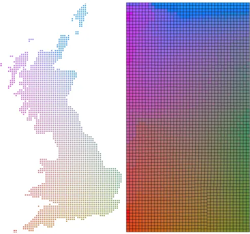
The coloring scheme is illustrated in Figure 8, which shows how a uniform distribution of grid squares over the landmass of Great Britain is represented as a non-hierarchical spatial treemap using the CIELab coloring scheme. Regions of color discontinuity can be seen where the landmass is least rectangular in shape (e.g. between North Wales and South West Scotland, and the far North East of Scotland).
3.2 Identifying Displacement
[image:5.612.312.559.266.469.2]19/03/2008 18:27 gridCentresCIELab.txt
Page 1 of 1 file:///Users/jwo/data/ordnanceSurvey/gb/gridCentresCIELab.svg
19/03/2008 18:48 Tree map
[image:6.612.57.303.48.278.2]Page 1 of 1 file:///Users/jwo/java/treeMaps/data/gridSquares.svg
Fig. 8. Ordnance Survey National Grid square centroids in their geo-graphic location (left) and as a non-hierarchical spatial treemap. The same CIELab color scheme is used for both images.
3.2.1 Numeric Measures
An obvious numeric metric is the average distance by which nodes have been displaced in order to tessellate their enclosing rectangle. This was calculated as follows:
dispDIST=
∑ni=1di
n√Aroot
(1)
Wheredi is the Euclidean distance between each node’s treemap
centroid and its affine transformed geographic location (to fit inside its enclosing node),nis the number of nodes andAroot is the area of
the root node. This provides a dimensionless ratio scaled between 0 (no spatial displacement) and 1 (maximum possible displacement).di
is always calculated relative to each node’s immediate parent node so as to avoid double counting of nodes which may be displaced simply because their parent was itself displaced.
Average length of displacement hides other potentially important geographical relationships. For example, it is possible to displace two nodes by only a small amount, but to change their topological and directional relationship with each other. Likewise, nodes may be dis-placed by large amounts, but if many local nodes are all disdis-placed together, their spatial relationship with each other may be preserved. Therefore, to complement the distance displacement measure, we can quantify the angular displacement between pairs of nodes. This can be calculated by taking the average angular deviation between pairs of nodes in treemap space and the same pairs in geographic space:
dispANG=
1
n2
n
∑
i=1
n
∑
j=1
acos ui j
ui j
·vi j vi j
!
(2)
whereui jis the vector between each leaf node and each of its
sib-ling leaves in treemap space,vi jis the same vector in geographic space
andnis the number of sibling leaves. The measure is scaled between 0 (no angular distortion by the treemap) and 180◦(equivalent of rotating the geographic space by 180◦about its centre).
Both the distance and angular metrics can be used to compare dif-ferent spatial arrangements of the same set of nodes, but should be used with more caution when comparing different sets of nodes since average displacement will depend in part on how regularly spaced the geographic locations of sibling nodes are. These displacement met-rics provide a useful indicator of average distortion and were used to
Table 3. Layout statistics for spatial layouts of trial datasets. ‘Simulation’ represents the mean of 1000 realizations of 100 log-normal randomly
sized nodes with Gaussian locations; ‘France’ represents the 95
de-partementsshown in Figure 6; ‘OSGB’ represents the Ordnance Survey National Grid squares shown in Figure 8; ‘US Population’ represents the US states sized according to population shown in Figure 9.
Dataset Layout Aspect ratio DispDIST DispANG
Simulation Spatial 2.66 0.21 24.3 Simulation HistoMap 2.88 0.37 62.2
France Spatial 1.14 0.15 18.9 France HistoMap 1.37 0.13 12.5
OSGB Spatial 1.02 0.19 14.1
OSGB HistoMap 1.32 0.19 14.2
US Population Spatial 2.26 0.17 22.1 US Population HistoMap 7.73 0.16 17.0
compare the effect of minor changes to the spatial layout algorithm as well as comparison with the geographicHistoMaplayout of
Mans-mannet al[17]. The results for the spatial layout and the HistoMap
for simulated and real geographic datasets are shown in Table 3. Both spatial layout algorithms perform best on distributions of nodes that are more regularly spaced and evenly sized (e.g. France and OSGB). The simulation datasets were deliberately constructed to chal-lenge the layout algorithms, with a Gaussian spatial distribution giving rise to a highly dense central region of nodes that require significant displacement to tesselate. The average aspect ratios for these data were sufficiently low to allow area-based comparisons, although the average figure does hide some small nodes with very poor aspect ratios. Dis-tance displacement is poorer for theHistoMaplayout than thespatial
layout, but angular displacement much poorer for theHistoMap lay-out. This suggests that for spatial distributions with high central den-sities and few spatial outliers, thespatiallayout may be more appro-priate. Distance and angular displacement tends to be slightly better when applying theHistoMaplayout to France and the US Population. This appears to be due to the fact that this layout (based on the pivot algorithm [2]) processes central nodes first and so is less affected by irregular peripheral distributions (e.g. the Brittany peninsular of NW France and the small population states of the E and NE United States).
3.2.2 Graphical Indicators
Numerical measures provide some insight into the qualities of the spa-tial tesselation of nodes, but they may fail to detect some systematic distortions that can result in misleading interpretations. We therefore propose using a visual indication of distance, directional, and topolog-ical distortion of geographic nodes by overlaying displacement vectors on the treemap. The displacement vector connects each treemap node to its affine transformed geographic location. In order to avoid clutter-ing the visual display, the quadratic Bezier arrow technique of Fekete
et al[11] was adopted. Here the connecting vector is represented as a
curve with greater curvature at the treemap node end of the line. Un-like [11], we set a single Bezier control point to 60◦to the right of the vector, at a distance of 25% of the vector length giving a straighter line than Feketeet alproposed. This tends to keep the displacement vector within the bounds of the enclosing rectangle while still indicating the direction of the displacement. By having the maximum curvature at the treemap node end of the vector, a stronger visual indicator of any spatial clustering is given. For treemaps with relatively small numbers of nodes, these vectors can be used as additional references to aid inter-pretation. For those with many nodes, the vectors can be used to give a general impression of where spatial distortion is greatest and weakest. They also provide additional information on the geographic layout of data while still allowing interpretation of the treemap hierarchy [24].
[image:6.612.324.558.125.245.2]car-togram of the United States. The vectors distinguish between the west-ern states where displacement in the treemap is uniformly towards the SE and the more complex distortion of the Eastern states where larger differences in size (population) and spatial distribution lead to some crossing vectors. In any variation of the squarified layout, relatively large nodes tend to force themselves towards the edge of their enclos-ing rectangle. This is because once a large node has been added, fur-ther smaller nodes added to the same row or column would have a very high aspect ratio and are therefore rejected. This is a problem for geographic patterns where the variable mapped to size is greatest towards the geographic centre of the space being mapped and signifi-cantly smaller at the periphery (see, for example, the effect of Michi-gan on Rhode Island, New Hampshire and Delaware in Figure 9).
26/03/2008 16:34 Tree map
Page 1 of 1 file:///Users/jwo/java/treeMaps/data/usPopulation.svg
Texas Montana
California New Mexico Nevada
Arizona
Michigan
Oregon
Colorado Wyoming
Minnesota
Idaho
Utah
South Dakota
Kansas North Dakota Washington
Nebraska
Wisconsin
Missouri
Oklahoma
Iowa Illinois
New York
Georgia Arkansas
Florida Alabama
Pennsylvania
North Carolina
Ohio
Mississippi
Louisiana Tennessee Kentucky
Virginia Indiana
Maine
South Carolina West Virginia
Vermont
New Hampshire
Maryland Massachusetts New Jersey
Connecticut Delaware
[image:7.612.61.280.192.342.2]Rhode Island DC
[image:7.612.60.280.501.705.2]Fig. 9. US Population 2006 by State showing spatial displacement of nodes as quadratic Bezier vectors. Nodes are sized by absolute popu-lation and colored according to popupopu-lation change.
Figure 10 shows the 2860 landmass nodes of the OSGB 10km grid squares laid out with thespatialandHistoMapalgorithms. The dis-tortion vectors provide a visual indication of where displacement is greatest and where it is most inconsistent. Crossing vectors result in darker regions and show where there is inconsistency in spatial distor-tion. By combining the images with the CIELab coloring of absolute position, artifacts of the pivoting process in theHistoMaplayout can be seen as discontinuities of color at 1/2n intervals. When used in a hierarchical treemap this has the potential to be confused with genuine hierarchical classification of data.
Fig. 10. OSGB grid squares showing spatial distortion of thespatial
(left) and HistoMap(right) layouts. Nodes colored using the CIELab
color scheme described in Section 3.1
4 CASESTUDY: PHOTOGRAPHMETADATAANALYSIS
To explore the suitability of ordered treemaps for information visual-ization we have applied both thespatialandordered squarifiedlayouts to the analysis of photographic landscape image retrieval. The work is built upon the research problem and approach identified by Edwardes and Purves [8] and Dykeset al[7] who investigated the metadata peo-ple choose to attach to photographic images of landscape when sub-mitted to public image archives. The purpose was to try to identify
howplaceis captured in volunteered geographic information [8, 12].
This work attempted to classify photographs according toscene types
which were further subclassified intoscene type descriptors, derived from the Pansofsky-Shatford facet matrix for image classification [20] and Smith and Mark’sgeographical kinds[26]. These classes were ex-tracted by performing textual analysis on photograph metadata such as titles, descriptions, tags and comments [8]. Because each photograph was of a located scene, part of that analysis involved investigating ge-ographic patterns in the way photographs are described.
The Flickr photo sharing service (www.flickr.com) was used to ex-tract the metadata for all photos that had been geolocated in the British Isles and contained at least one of the following scene types as tags:
mountain,hill,village,beach. Photos were then subclassified
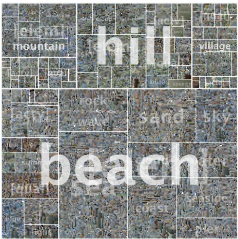
accord-ing to scene types divided into the followaccord-ing classes:elements(nouns such as peak, church, sand),qualities(usually adjectives such as cold, green, rural), andactivities(verbs such as walking, surfing, fishing). Selecting only photos with a geolocation accuracy of approximately 5km or better (Flickr accuracy levels 13-16), and filtering out those with ‘tag spam’, resulted in a set of ˜50,000 photographs tagged by the four scene types. Figure 11 shows the spatial treemap of these data se-lecting the 10 most frequent scene type descriptors for each category of scene type descriptor in each scene type. This yields a tree structure of depth 3, with 4 categories at the first level, 12 at the second and 120 at the third.
Positioning of non-leaf nodes gives a general view of relative ge-ographical patterns in subject matter and tagging behavior. So, for example, photos tagged with ‘mountain’ tend to be further north-west than those tagged with ‘hill’. Color can be used to identify the de-gree to which such relationships exist, for example that ‘beach/surf-ing’ tends to have a greater proportion of photographs in the SW than ‘beach/waves’. The displacement vector overlays in this context in-dicate the geographic concentration of photographs. This is most clearly seen in the ‘sea’ nodes where photos are inevitably concen-trated around the UK coastline. The ‘beach/pier’ node shows the dom-inance of Brighton pier in the south-east. The size of non-leaf nodes gives an indication of relative popularity of tag styles. So for example, elements are more common than qualities and activities for all scene types, with the contrast being strongest in photographs tagged with ‘beach’. Activity tags are more common than quality tags for hills and mountains but not for villages and beaches. The combination of vec-tor overlay and coloring of leaf nodes is useful in identifying where individual contributions or events can dominate a pattern (and could therefore be filtered out in further analysis). For example, the brown ‘car’, ‘hillclimb’, ‘racing’ and ‘carracing’ tags in the ‘hill’ scene type are dominantly taken by an individual at the Prescott Hill motor racing circuit in Southern England.
It is possible that direct analysis of submitted photographs in ad-dation to their volunteered metadata may help to identify what it is that contributors use to define place. Figure 12 shows the mean im-age color of each of the 50,000 photographs classified by scene type and scene type descriptor. Using the spatial layout it is possible to explore whether there are any geographic patterns in this color varia-tion. Figure 12 suggests that scene type descriptor is probably more strongly correlated with photo color than geography (e.g. hills are greener than any other scene type; most color quality tags are associ-ated with the color they describe, but ‘white’ and ‘light’ tagged photos appear darker than ‘black’ tagged photos. Where spatial layout does play a useful role is in identifying spatially clustered photos of a simi-lar average color. These tend to be multiple photographs submitted by the same contributor of the same event.
Fig. 11. UK Flickr photos categorised by scene type (beach, hill, mountain, village) and scene type descriptor (e.g. sky, blue, winter, surfing) with absolute location shown with spatial displacement vectors and color.
colored pixels though, as the ordering itself can affect the impression of the distribution of colors. The six treemaps shown in Figure 13 all show exactly the same data, but re-ordered according to different criteria and layout algorithms. The top row of Figure 13 shows a sub-graph of the tree where leaf nodes have been ordered using the
or-deredSquarifiedlayout. In each of the three examples, the same set
of mean colors have been ordered according to the 3 principal compo-nents of the RGB color space. The first component is approximately a transect though color value, the second along a blue-orange transect and the third along a green-magenta transect. A very different visual impression of the same set of colors can be given simply by chang-ing the (arbitrary) orderchang-ing of colored nodes. The bottom row shows the same nodes ordered by just the first principal component of color, but laid out using thesquarified,pivot by middleandstrip map algo-rithms. In each of these cases, discontinuities in color can be seen that don’t reflect properties of the data, but rather artifacts of the layout algorithm. These include localized clusters of orange and blue nodes, diagonal clusters of dark pixels and apparently nested square clusters that simply reflect the pivot points used in the layout algorithm.
5 CONCLUSION
We have proposed a pair of new algorithms that attempt to increase the cognitive plausibility of treemap layouts by relating the two-dimensional positioning of nodes in a treemap more closely to the properties of the data they represent. While attempts to do this have been made in the past, most notably by Bedersonet al[2], they have tended to focus on the problem of identifying a particular node within an ordered list. In our work, we have attempted to lay out nodes to allow trends and comparisons between nodes to be made. The geog-raphy of data is one obvious example, exploited by ourspatial
lay-out, where location is an important property that should be reflected in the information graphic. Where geographic information is not avail-able, we argue that theordered squarifiedlayout follows the distance-similarity metaphor more closely by minimizing arbitrary spatial dis-continuities that do not reflect properties of the data.
We have considered a number of metrics that might be used to mea-sure the success of a layout algorithm. We argue that readability, while summarizing the cognitive effort required to follow an ordered sequence of nodes, does not necessarily reflect the effort required to assess trends or comparisons between nodes. Instead we have used correlation between node order and distance from the origin of a par-ent node. For spatial layout of data with a geographic componpar-ent, measures of distance and angular displacement can be used to assess the degree to which the treemap reflects the spatial properties of the data it represents. This has allowed us to make comparisons between
ourspatiallayout and theHistoMaplayout [17], identifying the types
of spatial pattern that are best represented by each layout. Yet sum-mary statistics of overall spatial distortion or consistency fail to detect the impact of discontinuities in layout. These may be better reflected by graphical means such as displacement vectors and spatial color-ing. We have used these techniques to identify the spatial patterns and complex geographies of volunteered photographic metadata as well as drawing attention to the advantages of thespatiallayout over pivot-based algorithms.
Fig. 12. Categorized UK Flickr photos with color representing the mean color of the photograph represented by each leaf node.
Fig. 13. Selected treemap nodes showing six orderings of mean photo
color. Top row: Nodes ordered by the three principal components of
image color arranged using theOrderedSquarifiedlayout.Bottom row:
Nodes ordered by the first principal component of color arranged using thesquarified(left),pivot by middle(centre) andstrip(right) layouts.
ACKNOWLEDGEMENTS
GB outline (Figure 7) and National Grid squares (Figures 8 and 10), crown copyright/database right 2008. An Ordnance Survey/EDINA supplied service. The authors are also grateful for insightful discussion with Ross Purves and Alistair Edwardes at the University of Zurich on the use of treemaps for photographic image retrieval.
REFERENCES
[1] T. Barlow and P. Neville. A comparison of 2-d visualizations of hierar-chies. IEEE Symposium on Information Visualization, pages 131–138, 2001.
[2] B. B. Bederson, B. Shneiderman, and M. Wattenberg. Ordered and quan-tum treemaps: Making effective use of 2d space to display hierarchies.
ACM Transactions on Graphics, 21:833–854, 2002.
[3] C. Brewer. Guidelines for selecting colors for diverging schemes on maps.Cartographic Journal, 33:79–86, 1996.
[4] C. Brewer. Selecting good color schemes for maps.
www.colorbrewer.org, 2002.
[5] M. Bruls, K. Huizing, and J. van Wijk. Squarified treemaps.Proceedings
of the Joint Eurographics and IEEE TCVG Symposium on Visualization,
pages 33–42, 2000.
[6] N. Cawthon and A. V. Moere. The effect of aesthetic on the usability of data visualization.11th International Conference on Information
Visual-ization (IV ’07), pages 637–648, 2007.
[7] J. Dykes, R. Purves, A. Edwardes, and J. Wood. Exploring volunteered geographic information to describe place: Visualization of the ‘geograph british isles’ collection. In D. Lambrick, editor,GISRUK 2008, pages 256–267, Manchester, UK, 2008. Manchester Metropolitan University. [8] A. Edwardes and R. Purves. A theoretical grounding for semantic
de-scriptions of place. 7th International Symposium on Web and Wireless
Geographic Information Systems, 4857:106–121, 2007.
[9] S. Fabrikant. Cognitively plausible information visualization. In J. Dykes, A. MacEachren, and M.-J. Kraak, editors,Exploring Geovisualization, pages 667–690, London, 2005. Elsevier.
[10] S. Fabrikant, D. Montello, M. Ruocco, and R. Middleton. The distance-similarity metaphor in network-display spatializations.Cartography and
Geographic Information Science, 31:237–252, 2004.
[11] J.-D. Fekete, D. Wang, N. Dang, A. Aris, and C. Plaisant. Overlaying graph links on treemaps. InInfoVis03, pages 82–83, 2003.
[12] M. Goodchild. Citizens as sensors: the world of volunteered geography.
GeoJournal, 69:211–221, 2007.
[13] S. Jayaram, S. Schmugge, M. Shin, and L. Tsap. Effect of colorspace transformation, the illuminance component, and color modeling on skin detection. InCVPR’04, pages 813–818, 2004.
[14] B. Jenny and L. Hurni. Swiss-style colour relief shading modulated by el-evation and by exposure to illumination.Cartographic Journal, 43:198– 207, 2006.
[15] D. A. Keim. Enhancing the visual clustering of query-dependent database visualization techniques using screen-filling curves. Proceedings of the IEEE Visualization ’95 Workshop on Database Issues for Data Visualiza-tion, pages 101–110, 1995.
[16] A. MacEachren, C. Brewer, and L. Pickle. Visualizing georeferenced data: Representing reliability of health statistics.Environment and
Plan-ning A, 30:1547–1561, 1998.
[17] F. Mansmann, D. A. Keim, S. C. North, B. Rexroad, and D. Sheleheda. Visual analysis of network traffic for resource planning, interactive mon-itoring, and interpretation of security threats. IEEE Transactions on
Vi-sualization and Computer Graphics, 13:1105–1112, 2007.
[18] V.-E. Neagoe. An optimum 2d color space for pattern recognition. In
IPCV’06, volume 2, pages 526–532, Las Vegas, 2006. CSREA Press.
[19] P. Robertson and J. O’Callaghan. The generation of color sequences for univariate and bivariate mapping. IEEE Computer Graphics and
Appli-cations, 6:24–32, 1986.
[20] S. Shatford. Analyzing the subject of picture: A theoretical approach.
Cataloging and Classification Quarterly, 6:39–62, 1986.
[21] B. Shneiderman. Tree visualization with tree-maps: 2-d space-filling ap-proach.ACM Transactions on Graphics, 11:92–99, 1992.
[22] B. Shneiderman. Treemaps for space-constrained visualization of hierar-chies.www.cs.umd.edu/hcil/treemap-history, 2006.
[23] B. Shneiderman and M. Wattenberg. Ordered treemap layouts. In
Info-vis01, pages 73–78, 2001.
[24] A. Skupin and S. Fabrikant. Spatialization methods: A cartographic re-search agenda for non-geographic information visualization.
Cartogra-phy and Geographic Information Science, 30:99–119, 2003.
[25] smartmoney.com. Map of the market, 2008.
[26] B. Smith and D. Mark. Geographical categories: an ontological investiga-tion.International Journal of Geographic Information Science, 15:591– 612, 2001.
[27] W. Tobler. Thirty five years of computer cartograms.Annals of the
Asso-ciation of American Geographers, 94:58–73, 2004.
[28] Y. Tu and H.-W. Shen. Visualizing changes of hierarchical data using treemaps.Visualization and Computer Graphics, IEEE Transactions on, 13:1286–1293, 2007.
[29] H. Wainer and C. M. Francolini. An empirical inquiry concerning human understanding of two-variable color maps. The American Statistician, 34:81–93, 1980.
[30] C. Ware. Color. Information visualization: Perception for design, pages 97–144, 2004.
[31] R. Williams. Circle packings, plane tessellations, and networks. The
Geometrical Foundation of Natural Structure: A Source Book of Design,
pages 34–47, 1979.
[image:9.612.45.296.323.454.2]