Robust control design using quantitative feedback theory

      

City, University of London Institutional Repository

Citation

:

Nandakumar, R. (2008). Robust control design using quantitative feedback theory. (Unpublished Doctoral thesis, City University London)

This is the accepted version of the paper.

This version of the publication may differ from the final published

version.

Permanent repository link:

http://openaccess.city.ac.uk/19631/

Link to published version

:

Copyright and reuse:

City Research Online aims to make research

outputs of City, University of London available to a wider audience.

Copyright and Moral Rights remain with the author(s) and/or copyright

holders. URLs from City Research Online may be freely distributed and

linked to.

City Research Online: http://openaccess.city.ac.uk/ [email protected]

ROBUST CONTROL DESIGN USING

QUANTITATIVE FEEDBACK THEORY

By

Ramnath N andakumar

A Dissertation submitted for the degree of

Doctor of Philosophy

Supervisor:Dr.George Halikias

City University

School of Engineering

&

Mathematical Sciences

Control Engineering Research Centre

Northampton Square,

London, EC1V OHB

IMAGING SERVICES NORTH

Boston Spa, Wetherby West Yorkshire, LS23 7BQ

www.bl,uk

THE FOLLOWING HAVE BEEN REDACTED AT THE

REQUEST OF THE UNIVERSITY

Declaration

I Ramnath Nandakumar, hereby certify that this thesis been written by me, that it is the record of work carried out by me and that it has not been submitted for any other higher degree qualification.

Contents

Declaration

Notation

Abbreviations

1 Introduction 1.1 Thesis outline

1.2 Thesis Contribution.

1.3 Publications resulting from this work

2 Literature Survey

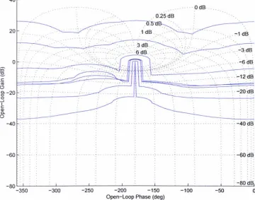
3 Design Background 3.1 Nichols Plot . . .

3.1.1 M-Circle 3.1.2 N-Circles.

3.1.3 Transfer of M circles to Nichols Plot 3.2 S t a b i l i t y . . .

3.2.1 Nyquist Stability Criterion.

3.2.2 Stability criterion on the Nichols Chart 3.3 Uncertainty . . . .

3.3.1 Parametric Uncertainty. 3.3.2 Frequency Domain

4 QFT Design

4.1 Design Specification. 4.2 Uncertainty Templates

4.2.1 U-Contour. 4.3 Tracking Bounds .

4.4 Disturbance Rejection . 4.5 Disturbance Bounds B D 4.6 Loop-Shaping . . . . 4.7 Pre-Filter . . . . .. 4.8 M ultivariable system

5 Loop-shaping

6

5.1 Linear Programming 5.2 Bode integral . . . .

5.2.1 Derivation ..

5.2.2 Approximate Discretisation of Bode's integral 5.3 Analytic constraints . . .

5.4 Fixed-structure controllers 5.4.1 Introduction . . . . 5.4.2 Problem description

5.4.3 Formulation of QFT constraints as frequency-dependent inequal-ities

...

5.4.4 Optimisation algorithm . 5.4.5 Optimisation algorithm steps: 5.4.6 Design example

5.5 Conclusions

...

QFT Software Toolbox 6.1 Introduction . . . . . 6.2 Template Generation

6.2.1 Algorithm Pseudo-Code 6.3 Convex Hull . . . .

6.3.1 Algorithm Pseudo-Code 6.4 Horowitz Bounds (Tracking) . .

6.4.1 Algorithm Pseudo-Code 6.5 Disturbance rejection bounds

6.5.1 Algorithm Pseudo-Code

6.6 High Frequency Contour (U-Contour) .

6.6.1 M-Circle . . . 6.6.2 Algorithm Pseudo-Code 6.6.3 Algorithm Pseudo-Code 6.7 Graphical Stability

...

,

...

6.8 Stability criterion . . . 125

6.8.1 Nyquist Stability criterion 125

6.8.2 Stability criterion on the Nichol's Chart 125

6.9 Graphical design . . . . 127

6.9.1 Nyquist Criterion 127

6.9.2 Nichol's Criterion 128

6.9.3 Algorithm Pseudo-Code 128

6.10 Loop Shaping . . . 130

6.10.1 Manual loop-shaping tool 131

6.10.2 Fixed-structure controller optimisation 133

6.11 Pre-Filter . 136

6.12 Conclusions 136

7 Case study - Design of hydraulic actuator 137

7.1 Introduction... 137

7.2 Background and General Design Objectives 138

7.3 Modelling of Hydraulic actuator interacting with environment 140

7.4 Uncertainty modelling and QFT Control Design 148

7.5 Conclusions . . . 158

8 Conclusions, Future Work 160

8.1 Conclusions 160

8.2 Limitations 162

8.3 Future Work. 162

Bibliography 164

9 Appendix I

9.1 Appendix A I

9.2 Appendix B III

9.3 Appendix C VIn

9.3.1 M-file to demonstrate controller design using QFT method. . VIII 9.3.2 M-file to demonstrate Bode approximation.. . . XIV 9.3.3

9.3.4 9.3.5 9.3.6

The function used to generate the uncertainty templates M-file to generate the convex hull with the sub function. M.file to calculate the Horowitz templates

M.file to calculate disturbance bounds .,

4

9.3.7 M-file used to construct M-contours in the Nichol's chart. 9.3.8 M-file to construct high-frequency bounds .

9.3.9 M-file to check Nichols stability criterion .. 9.3.10 M-file to design the optimum PID controller 9.3.11 M-File for graphical design of the controller 9.3.12 M-file to design the Pre-filter

9.4 Appendix D . . . .

List of Figures

1.1 Feedback Configuration . 5

3.1 M circle on Nyquist Plot 19

3.2 M circle for Casel, Case2 and Case3 20

3.3 M circle for M

>

1 . . . 22 3.4 M circle when M = 1 . . . 23 3.5 M circle on Nichols Plot for M

>

1, Al < 1, M = 1 23

3.6 M circle when M

<

1 24

3.7 Nichols Plot 25

3.8 S - Plane . 27

3.9 Positive and Negative crossing, and stability lines Be and Bn on the Nyquist plane and Nichols chart . . . 30 3.10 Stability region shown on Nichols chart, Fig (a) A. One crossing B. No

corssing, Fig (b) Several crossings. . . . 31 3.11 Plant with Additive fig( a) and Multiplicative fig(b) Uncertainty's 35

3.12 Parameter Uncertainty . . . . 36

3.13 Uncertainty Represented on Nyquist plot 37

4.1 Bounds on step response of the plant . . 42 4.2 Bounds on the magnitude and phase responses of the plant 42 4.3 Modified bounds on plant step response . . . . 43 4.4 Modified bounds on magnitude and phase responses 44 4.5 Parameter Uncertainty . . . . 46

4.6 Uncertainty Template . . . . 46

4.7 Nominal Open-loop and Uncertainty Templates. 48

4.8 M-circle in Nyquist plane (M> 1) . . . 49 4.9 M-circle and U-contour in Nichols chart (M> 1) 51 4.10 U -contour . . . . 52

4.11 Tracking Bound placements on the Nichols chart uszng Uncertainty

Templates . . . . 54

4.12 Horowitz Bounds 55

4.13 Step response for Md 58

4.14 Bode plots for Md . . 58

4.15 Disturbance bounds BD 60

4.16 Overall bounds. . . . . 60

4.17 Loop-shaping phase correction 64

4.18 Final Loop-shaping . . . . 65

4.19 Step response of the system with the Pre-filter and controller in cascade 66

4.20 Frequency response of the closed-loop system 67

4.21 General Multivariable system . 67

4.22 Expanded Multivariable system 68

4.23 General feedback control system . 69

4.24 Expanded Multivariable system 70

5.1 Differentiability region . . . .

5.2 Phase reconstruction for first transfer function .

5.3 Phase reconstruction for second transfer function

5.4 Differentiability region . . . .

5.5 Feedback Configuration. . . . 5.6 Curve N(¢) used to calculate closed-loop bandwidth 5.7 Optimal Loop-shaping with PID controller

5.8 Closed-loop system frequency response.

5.9 Step responses of plants . . . .

5.10 Disturbance rejection in the time domain

6.1 Nominal Open-loop and Uncertainty Templates.

75 80 80 82 84 90 104 105 105 106 110

6.2 Convex hull design . . . 112 6.3 Convex hull of the uncertainty template at six frequencies 113

6.4 M circle for Casel, Case2 and Case3 118

6.5 Phase regions on the Nichol's chart . 121

6.6 M circle on Nichol's Plot for M = 1.2, M

=

1 and M

=

0.8 123 6.7 M-circ1e and U-contour in Nichol's chart (M

>

1) . . . 124 6.8 Positive and Negative crossing, and stability lines Se and Sn on the

Nyquist plane and Nichol '8 chart . . . . 125 6.9 Stability region given on a Nichol's chart 127

6.10 Graphical test flowchart . . . 129

6.11 Lead/Lag-network manual loop shaping tool 132

6.12 Control Design with Lead/Lag Network. 133

6.13 Design with Optimal PID controller . . . 135

7.1 Diagram of the hydraulic actuator (based on [40]) 140

7.2 Manipulator-sensor-environment... 145

7.3 Closed-loop design tracking specifications, upper and lower bounds. 150 7.4 Uncertainty template, fifth design frequency . . 151 7.5 Uncertainty template, sixth design frequency. . 152

7.6 Uncertainty template, seventh design frequency 153

7.7 Nominal-plant frequency response, Horowitz templates and U-contour 154 7.8 Nominal open-loop response with P DD2-optimal controller. . . . .. 155 7.9 Nominal open-loop response with modified P DD2-optimal controller.

7.10 Shaped open-loop response and uncertainty templates. 7.11 Closed-loop frequency responses - No pre-filter .. 7.12 Closed-loop frequency responses - \Vith pre-filter. 7.13 Closed-loop step responses - With pre-filter.

9.1 Feedback Configuration. . . . 9.2 M-circle in Nyquist plane (M > 1)

9.3 M-circle and U-contour in Nichols chart (M > 1)

8

156 157 158 159 159

List of Tables

1. Magnitude and Phase values of corresponding frequencies

2. Values of l5(jWi) over 8 design frequencies

3. Open-loop for robust disturbance rejection

4. operating values and parameter range

5. Closed-loop specifications, Maximum and minimum gain

6. Target and achieved pre-filter gains

Notation

n,C,N Sets of real, complex and natural numbers

n( s ) field of rational functions in s with real coefficients n[s] the set of real polynomials in the variable s

81) Boundary of set 1)

U -contour Closed contour in Nichols chart If( <p) Horowitz templates

Il(

<p) Disturbance templates

JC Family of all stabilising controllers S Set of all stable closed-loop systems

T Set of all stable control sensitivity functions Ji,fp Maximum peak

tp Peak time

ts Settling time tT Rise time

Throughout this thesis matrix dynamical systems appear inside parenthesis so that they are distinguished from constant matrices which are denoted by square brackets.

Abbreviations

QFT PID PI LQR LQG CAD LMI LTI

Quantitative Feedback Theory

Proportional Integral and Derivative Controller Performance Index

Linear Quadratic Regulator Linear Quadratic Gaussian Computer Aided Design Linear matrix inequality Linear time invariant

MIMO Multiple input multiple output UHFB Universal High Frequency Bound

LP Linear Programming RHP Right Hand Pole

SISO Single input single output SSV Structured singular value SVD Singular value decomposition SIMO Single input multiple output

Abstract

Chapter

1

Introduction

In this work we develop robust control design techniques based on a methodology known in the literature as Quantitative Feedback Theory (QFT). This method, first introduced by 1. Horowitz [28] in the early 70's, applies to the control design of dy-namic systems which are subject (to potentially large) uncertainty in plant dydy-namics. QFT is a systematic procedure for designing systems of this type, and can guarantee "worst-case" performance and stability properties to the designed dosed-loop system, in the sense that these properties apply over the whole family of models describing the uncertain plant dynamics. This characteristic makes QFT a robust control design methodology.

QFT is essentially a loop-shaping design procedure. The design objectives are typically formulated in terms of bounds on the dosed-loop frequency response characteristics, which in turn can be translated to constraints on the open-loop frequency responses of the plant. The design requires shaping the open-loop frequency-response character-istics, so that these constraints are satisfied (over all frequencies). If the constraints are feasible, an appropriate optimality criterion is typically introduced, which allows the designer to select the "best" design by choosing the most appropriate feedback control scheme. In this sense, QFT is also an optimal control-design methodology, since loop-shaping is normally performed with this optimality criterion in mind. In this chapter the QFT design methodology is outlined for uncertain, linear, single-input single-output systems subject to typical stability and performance requirements. Be-fore this description, however, we introduce the main characteristics of the method by describing two important control-design methodologies, optimal and robust control.

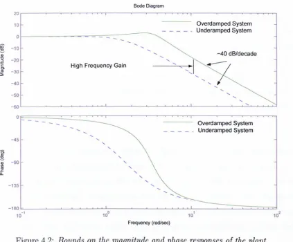
Optimal Control: Optimal control is a design approach which aims at getting the best possible performance out of a plant. This objective is normally achieved byoptimis-ing a mathematical expression which incorporates all aspects of the design which are deemed to be important, e.g. stability margins, performance objectives, etc. This ex-pression is called the performance index (P.L). The optimal controller is obtained by solving an optimisation problem, typically involving a number of constrains. One of the most successful optimal control methodologies was LQR/LQG (Linear Quadratic Regulator/Linear Quadratic Gaussian). In this method one assumes that the exoge-nous inputs (disturbances and noise signals) entering the system can be modelled as coloured or white noise signals, and minimises a quadratic performance index involv-ing the rms average power of the regulated variables, which typically include a linear combination of the state variables and the control signals. \Vhen all state variables are available for feedback, the optimal solution consists of an optimal state-feedback matrix which is calculated by solving an Algebraic Riccati Equation. When a number of (noisy) output signals (other than states) are available, the optimal solution is ob-tained via the separation principle and consists of an optimal state estimator (Kalman filter) combined with the optimal state feedback obtained using the LQR procedure. Although the LQR design has excellent robust stability properties (good guaranteed gain and phase margins), these are typically lost when a Kalman filter is employed. An optimal controller method which takes into account explicitly robust stability and performance requirements is Hoc - optimal control which was developed in the last two decades. This method shares many aspects of its philosophy with QFT; however, the performance index which is optimised is formulated in terms of the infinity norm of the closed-loop tranfer functions; this is in contrast to QFT design which optimises the open-loop frequency response characteristics similarly to classical control. Despite these differences, it is argued in this thesis that the two methods can fruitfully com-plement one another.

Robust Control: During the control design process it is typically assumed that the plant is represented by an linear time-invariant (LTI) model, typically obtained by linearising a non-linear process around a fixed equilibrium point. In practice, the plant is subjected to various changing conditions in its interactions with its environment which tend to move the plant's set point, and as a result the linearised model will also

change. Additional sources of uncertainty may be due to factors like wear and tear due to aging of components or due to changing environmental conditions. The plant may also encounter unaccounted external factors like disturbances, or its mathematical model may have errors arising due to lack of knowledge of the exact values of certain of its parameters by the designer, approximations made in the modelling process itself due to simplicity requirements, or inconsistencies in the transducers used to measure various signals used for feedback. A control system which is capable to accommodate the effects caused by all these uncertainty factors is called robust. In general, when it can be shown that the controller design is stable for all plants within a specified family which contains all possible sources of uncertainty ("model - uncertainty set"), then we say that the controller provides robust stability. Apart from robust stability, we are also interested in robust performance, i.e. the performance of the design should not degrade excessively when plant uncertainty is taken into account and control signals should be kept within realistic lever/rate bounds. Typically, robust design methods (including QFT) employ optimality criteria of a "minimax" type, i.e. they optimise the design for the "worst-case" situation (e.g. signal, parameter) that can occur among those allowed by the corresponding uncertainty model. This implies that "robust" control methods can be conservative, and care must be taken to describe the uncertainty set as accurately as possible.

Quantitative Feedback Theory is a systematic robust control design methodology for systems subject to large parametric or unstructured uncertainty. QFT is a graphical loop-shaping procedure, traditionally carried out on the Nichol's chart, which can be used for the control design of either 8180 or MIMO uncertain systems, including non-linear and time-varying models [17, 28, 57, 16]. Relative to other robust-control design methodologies, QFT offers a number of advantages, apart from its utilisation of clas-sical control-design techniques. These include: (i) The ability to assess quantitatively the "cost of feedback" [29], (ii) the ability to take into account phase information in the design process (this is ignored in many norm-based approaches, e.g. 7-lrXJ optimal con-trol which is based on singular values), and (iii) the ability to provide "transparency" in the design, i.e. clear tradeoff criteria between controller complexity and the feasibility of the design objectives. Note that (iii) implies in practice that QFT often results in simple controllers which are easy to implement.

The QFT design procedure is based on the two-degree of freedom feedback configura-tion shown in Figure 1.1. In this diagram G(p, s) denotes the uncertain plant, while K(s) and F(s) denote the feedback compensator and pre-filter, respectively, which are to be designed. Note that model uncertainty is described by the r-parameter vector pEP ~ Rr taking values in the set P; it is further assumed that G(p, s) has the same number of RHP poles for all pEP. Translating the uncertainty into the frequency domain, gives rise to the plant's "uncertainty templates" which are the sets:

Qw = {G(p,jw) : pEP}

For each fixed frequency w, Qw defines a "fuzzy region" on the Nichol's chart which describes the uncertainty of the plant at frequency W in terms of magnitude (in dB's) and phase (in degrees). For design purposes, we construct N uncertainty templates corresponding to a discrete set of frequencies {WI, W2, ... , W N} chosen to cover ade-quately the system's bandwidth.

The robust performance objectives of the design include good tracking of reference input r( s) and good attenuation of the disturbance signal d( s) entering at the system's output, despite the presence of uncertainty. The robust tracking objectives are captured by the set of inequalities:

I

G(p, jWi)K(jWi)

I

()

maxb. 1 G( . )K(·) ~ {} Wi := BU(Wi)ldB - BI(Wi)ldB

pEP

+

p, JWi JWi dB

for each i

=

1,2, ... ,N, i.e. if, for each frequency Wi, the maximum variation in closed-loop gain as pEP does not exceed the maximum allowable spread in specifications

{}(Wi), typically specified via two appropriate magnitude frequency responses Bu(w) =

IBu(jw)1 and BI(W) = IBI(jW)I. Note that it is not necessary to bound the actual gain (but only the gain spread) since we assume that, (i) no uncertainty is associated with the feedback controller K(s), and (ii) the pre-filter F(s) can provide arbitrary scaling to the closed-loop gain.

The robust disturbance-rejection objective can be satisfied by bounding the sensitivity function, i.e. by imposing constraints of the form

max

I

1

I

<

D( Wi)

pEP 1

+

G(p,jwi)K(jWi)

-for a (subset) of the design frequencies {Wl' W2 ... ,W N }. Again these are typically

d(s)

r(s) F(s) K(s) G(p,s)

Figure 1.1: Feedback Configuration

ified via an appropriate magnitude frequency-response D(w) = ID(jw)l.

Robust stability is enforced by ensuring that: (i) no unstable pole-zero cancellations occur between the plant and the controller (for every pEP), (ii) the nominal open-loop frequency response Lo(jw) = G(Po,jw)K(jw) (defined for any Po E P) does not cross the -1 point (i.e. the (-180°,0) point on the Nichols chart) and makes a total number of (anti-clockwise) encirclements around it equal to the number of unstable poles of Lo(s) = G(po, s)K(s), and (iii) no (perturbed) open-loop response crosses the -1 point, i.e.

-1 rJ-

U

K(jw)Qw

wEIR.

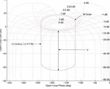
Note that condition (i) is automatically satisfied if K(s) is restricted to be stable and minimum-phase, while conditions (ii) and (iii) can be easily tested graphically [13, 12]. In practice, a more severe condition than (iii) is imposed: To establish a minimum amount of damping, it is required that the nominal open-loop frequency response does not penetrate a closed contour in the Nichol's chart (U-contour); this is constructed from an appropriate M-circle and information about high-frequency uncertainty ofthe plant [17, 28].

The robust tracking and disturbance rejection objectives have been formulated as gain inequalities of the closed-loop transfer functions (sensitivity and complementary sen-sitivity) at the design frequencies. For the purposes of QFT design, these inequali-ties must be translated into constraints on the nominal open-loop response Lo(jw).

This procedure results into a number of contours ("Horowitz templates"

Jf(¢)

and "disturbance-rejection templates" iid(cp)) for each frequency Wi, i = 1,2, ... , N; these

are functions of the phase variable ¢ E (-360°, 0°]. Thus, robust tracking is satis-fied at frequency Wi if ILo(jwd

IdB

~

Jl(

¢i) where arg Lo(jWi) = ¢i; similarly, robust disturbance-rejection is attained at frequency Wi if ILo(jWi)ldB ~ fl(¢). The robust-performance templates (Horowitz and disturbance-rejection) can be easily constructed (within an arbitrary gain tolerance and for a discretised phase-grid) using a simple bisection algorithm.

Once the contours corresponding to the robust stability and performance specifications have been defined, the design proceeds via loop-shaping. First, an arbitrary nominal plant Go(s) = G(po, s) is selected, corresponding to an arbitrary pEP. The open-loop frequency response characteristics of Lo(s)

=

KGo(s) are then shaped so that the robust stability and performance specifications are satisfied. This procedure is typically carried out by the designer in a CAD environment on the Nichols chart and requires a significant trial-and-error element. If the QFT constraints can be met, the best design is considered to be the one that requires as "little gain as possible". This requirement is formulated rather vaguely at present, but will be made precise in the sequel. Clearly, the objective here is to avoid an "over-design" of the system, by using higher gains than necessary. There are two main reasons for this requirement:

• A high open-loop gain implies a wide closed-loop bandwidth for the "complemen-tary sensitivity" functions:

T( p, s - --....::...;,-.:...,...:...;:,...,... ) _ G(p, s)K(s) 1

+

G(p, s)K(s)

Now note that the transfer function from a sensor noise input n(s) to the plant output y(s) is -T(p, s). Assuming that the spectrum of the sensor noise input is sufficiently "wideband", the larger the bandwidth of T(p, s), the more "noisy" the output signal will appear. Thus, to prevent a noisy output signal y(t) we need to restrict the bandwidth of T(p, s) and thus the system's open-loop gain .

• A more important reason for the open-loop gain and thus also the closed-loop bandwidth of T(p, s) is related to robust stability: For unstructured multiplica-tive perturbations, the robust stability margins are inversely proportional to IT(p, jw)

I.

Since high frequency unstructured perturbations are typically present in practical systems due to the loss of phase information at high frequencies, unmodelled high frequency dynamics, etc, it is always desirable to avoid

sive closed-loop bandwidths which may cause instability. Note than unstructured high frequency dynamics cannot be accounted by parametric uncertainty typi-cally used to describe uncertainty in the standard QFT framework, although it is possible to modify the approach to take it into consideration.

Due to these two reasons, an optimal QFT design should make use of the minimal amount of gain, i.e. just enough to meet the robust performance objectives. Thus, it is typically attempted to shape the open-loop frequency response of the system so that

L(jWi), i = 1,2, ... , N lies exactly on, or just above, the corresponding Horowitz tem-plates. This typically requires a significant amount of skill on the part of the designer and may be too difficult to perform adequately using a trial-and-error procedure. In the present work, it is attempted to alleviate this difficulty by automating the loop-shaping design procedure via a number of optimisation algorithms. These will be described in full in subsequent chapters of the thesis.

When an appropriate feedback controller has been designed, such that all robust stability and performance constraints are satisfied, the QFT procedure is concluded by designing a pre-filter to satisfy reference signal tracking specifications. This is typically a scaling exercise and can be performed using either a manual or an optimisation-based technique. Finally, closed-loop simulations are typically performed to validate the adequacy of the designed control scheme.

1.1

Thesis outline

The first chapter of the thesis outlines the QFT design procedure and formally defines the problem in an optimisation framework. The related areas of robust and optimal

control are also briefly reviewed. A brief literature survey of the work related to this project is included in Chapter 2, with particular emphasis to QFT-based control design methods.

Chapter 3 describes the basic background of the QFT approach, including its main motivation and the various analysis tools employed, with particular emphasis on those related to the description of model uncertainty and graphical stability tests.

In Chapter 4 the QFT design method is described in detail. A number of theoretical results related to the method are stated, along with various examples illustrating each step. Since it is common practice to carry out the design using the Nichol's chart, some related background material is also included. The emphasis of the exposition is on the development of novel CAD tools and algorithms which can assist the designer or automate altogether the more difficult steps of the procedure. A description of a number of such tools is included, and a number of known results are reformulated so that they can be checked automatically (e.g. robust stability conditions on Nichols chart).

Chapter 5 proposes two new controller design methods based on automatic loop-shaping techniques, and tests their effectiveness via design examples and simulations. In the first method, the robust performance objectives (arising from the Horowitz and U-contours) are used to define the set of linear constraints of the linear programme. These are augmented by another set of constraints (realisability, analyticity) which ensure that the optimal frequency response is realisable by an LTI dynamic system corresponding to the feedback controller. The second algorithm is related to the design of simple controllers of a fixed structure (PID, phase lead/lag, second-order). Here, the optimisation is carried out over the set of controller parameters.

Chapter 6 describes in detail the various steps of the complete set of QFT design al-gorithms, leading to the implementation of the software tool. This includes routines related to graphical representation of various contours in the Nichols chart (e.g. stabil-ity regions, robust performance contours, M-circles, plant uncertainty templates, etc), routines drawn from computational geometry (e.g. convex hulls) and various routines implementing optimisation algorithms, mainly related to automatic loop shaping and controller design.

In chapter 7 a detailed case study of a non-linear hydraulic actuator modelling a real system is presented. The model is linearised around an operating point and the uncer-tainty in the nominal plant is quantified in terms of ten uncertain parameters assumed to vary independently over their corresponding ranges. The methods developed in the thesis are used to design a robust QFT controller which meets the defined robust

bility and performance specifications. The design is validated via extensive simulations and direct comparison with designs reported in the literature [41] implemented on the real system.

The main conclusions of the thesis, together with an outline of the scope for future work are included in Chapter 8. Finally, the appendices appearing at the end of the report contain background material related to the project, derivations and proofs of various technical results, together with the Matlab software tool developed in this project.

1.2 Thesis Contribution

• The thesis develops novel optimization-based techniques for analysing and designing robust feedback controllers using the QFT method. Robust stability and performance bounds are represented as mathematical constraints and are subsequently used to formulate optimization problems and thus automate the loop-shaping design procedure. This replaces traditional design methods relying on manual loop-shaping which require expert knowledge from the designer and may result in sub-optimal control schemes.

• The emphasis throughout the work is to design simple-structure controllers which can be used in practical industrial control. This is consistent with the design philosophy of the QFT method and provides "transparency" to the design. Thus, more complex controllers are introduced only when simple structures are deemed to be inadequate in some sense.

• Part of the work described in the thesis develops a novel computer-based design environment for carrying out robust-control designs using the QFT method and for assessing their performance and stability properties. This is based on fusing together techniques from computational geometry and optimization. The environment can be used for the purposes of representing plant uncertainty, visualizing the problem constraints, carrying out manual and optimization-based feedback control designs and validating the properties of the resulting control schemes. All optimisation algorithms developed in this work have been successfully tested in this environment, along with a detailed case-study of a non-linear actuator.

1.3 Publications resulting from this work

• R. Nandakumar, G. Halikias and A. Zolotas, "An optimization algorithm for designing fixed-structure controllers using the QFT method", 2002 IEEE Inter-national Symposium on Computer Aided Control Systems Design Proceedings, Glasgow, Schotland UK, September 18-20 2002.

• R. Nandakumar, G. Halikias and A. Zolotas, "A new Educational tool for robust c control design using the QFT method" , Proc. of the 42nd IEEE Conference on Decision and Control, Vol. 1, pp. 803-808, 9-12 December 2003.

• R. Nandakumar, G. Halikias and A. Zolotas, "Robust Control Design of a

Hydraulic Actuator Using the QFT Method" Proc. European Control Conference 2007, no WeA10.4, Kos, Greece, July 2-5, 2007.

Chapter

2

Literature Survey

Quantitative feedback theory (QFT) was initially proposed by I.M.Horowitz in 1963 [28]. It is a design method for designing robust control systems for uncertain plants subject to structured, unstructured or mixed-type uncertainties. QFT was initially developed for SISO systems and later extended to the multi variable case. The main contribution of Horowitz's work was to formulate the loop-shaping problem for an un-stable and/or non-minimum phase plant and show that this is equivalent to a problem involving a stable non-minimum phase plant, by appropriately re-defining its robust stability and performance bounds. Initially, the proposed design procedure did not involve unstable plants; however this procedure was later extended by Horowitz to the unstable case in [30]. In 1972 Horowitz and Sidi proposed a new procedure for car-rying out the robust control feedback design, by shifting the plant's stability bounds [29]. Although this procedure was generally efficient it lacked a formal proof, an issue that was successfully addressed by Chen and Ballance [12]. The QFT technique was extended to SIMO systems by Breiner [5].

non-minimum phase and unstable systems. Their work resulted in a simple test which can be verified automatically via purely graphical means. This is especially useful for QFT design within a automated CAD environment and is used extensively in this work.

Although the main objective of the QFT design is to achieve robust stability, it is also important to satisfy robust performance specifications. In QFT these are typically imposed in the form of frequency-domain bounds on the sensitivity, complementary sensitivity and control-sensitivity functions, over a discrete frequency grid. The robust performance objectives are normally regarded as the constraints of an optimisation problem, the optimality criterion being formulated in terms of system over-design and controller complexity. Thus, the optimal loop-shaping of the open-loop characteris-tics becomes a significant aspect of the design, i.e. identifying the design (among all

"feasible" designs) which achieves an "optimal" solution for the system. Design of ro-bust controllers using QFT for plants with uncertainty was investigated by Jayasuriya and Zhao [32, 33]. Sidi [44, 45] and Horowitz and Sidi [30] presented a robust con-trol design method for uncertain non-minimum phase plants with required closed-loop performance. No explicit optimisation problem was formulated; however their method gives the designer valuable insights into the tradeoff between closed-loop performance and bandwidth limitation [29]. A solution to the control problem is achieved during the loop-shaping stage of the procedure, using geometric contours derived from the robust performance specifications and the description of plant uncertainty. This essen-tially involves a modification of the open-loop response of the system, required to lie in certain regions of the Nichols chart and specified by the geometric contours described above. [36] provides a method for designing non-minimum phase MIMO system.

In the procedure initially suggested by Horowitz, manual loop-shaping was used. This is performed via an iterative design procedure and requires considerable skill from the part of the designer. Manual loop-shaping is essentially a trial and error method. Consequently, if the graphical constraints seem infeasible, it is not possible to decide conclusively whether this is due to the simple structure of the controller used, to the limitation of the designer's abilities, etc.

After the arrival of computers capable of carrying out complex calculations, a

icant amount of effort has been devoted in trying to develop automatic loop-shaping QFT procedures. Polygonal approximation of the uncertainty templates was employed by Longdon and East (1978). A similar computational technique applicable to non-rational transfer functions aiming to alleviate the construction of uncertainty templates of QFT was reported by Gautam and Natarai [22]. Template generation using param-eter discretisation methods suffers from the "curse of dimensionally". As a result in most problems the designer is forced to trade-off between choosing a coarse plant grid to minimize the computational burden versus a fine grid to maintain highly accurate robustness specifications. An attempt to alleviate this problem using methods not re-lying on gridding is proposed in [4].

Another fundamental problem of QFT involves the design of the feedback controller satisfying satisfies a discrete set of robust stability and performance specifications. Yaniv and Chait [61] proposed a design method using quadratic inequalities, which applies both to continuous and discrete-time systems. A technique based on including a measure of unstructured uncertainty, the amount of which is dictated by the circle criterion, was proposed by Wang [55]. An efficient design technique was first obtained by Gera and Horowitz [24]. An automatic loop-shaping algorithm using convex opti-misation which optimises the location of the zeros of the controller was proposed by Chait [9]. This has the clear limitation that the denominator of the controller must be specified in advance. Certain ad hoc rules for this task have been proposed in [9], but these require significant skill and experience from the part of the designer. The single-loop feedback design technique by Horowitz and Sidi [29], matches sensitivity as well as robustness specification for the exact amount of model uncertainty, and its criterion for a good design is the high-frequency gain originating by the ideal Bode characteristic of a loop transmission function [2]. An adaptive algorithm to modify the controller's parameters by reducing the effects of plant uncertainty without affecting closed-loop performance was proposed by Yaniv [56]. Gutman [26] developed an algo-rithm to identify the reduced plant uncertainty.

reconciling QFT and robust multivariable control was proposed by [48] using an ap-proximation technique. Using this method it was shown that Nichols chart robustness bounds can be calculated without gridding of the uncertainty set and instead can be approximately solved using standard tools of robust multivariable control. Further connections between QFT and modern robust control were established by Lee, Chait and Steinbuch [37]. In this work it is argued that the integration of optimal control synthesis and manual tuning in QFT design environment enables design of controllers with levels of performance that surpasses what can be achieved using only a single technique. A constructive example is used to demonstrate that QFTs open-loop tun-ing can be more transparent than tuntun-ing closed-loop weights, as in modern robust control. Another approach aiming to develop a design methodology by utilising the best features from both modern robust control and QFT is proposed in [1]. In con-trast to QFT, modern robust control typically results in high-order (observer-based) controllers. In the above cited work the authors characterise a class of second-order three-parameter controllers (including PID and lead/lag compensators) satisfying given 1ioo norm closed-loop specifications using simple geometric considerations. An exam-ple illustrating the method is applied to the design of a PID controller in the case of bounded sensitivity specifications. These results were extended in [35] to the problem of obtaining the complete set of PID parameters that attains prescribed gain and phase margins.

aspects of QFT-based methodologies are reported by [51], who also show that QFT design can be formulated as a "strong" 'Hoo optimisation problem.

Thompson and Nwokah [51] developed an algorithm for shaping minimum-gain con-trollers. A more recent trend in automatic loop-shaping involves the use of convex optimisation methods. Bryant and Halikias [6] introduced a design procedure based on

linear-programming. Another method of optimal loop-shaping involving simple fixed-structure controllers was proposed by Zolotas and Halikias [63]. The last two methods (linear programming approach and fixed-structure controller optimisation) are devel-oped further in this work. Gain-bandwidth optimisation methods of PID controllers in the context of QFT design are also developed in [53]. [53] also describes a constrained optimisation method aimed at reducing the excess gain-bandwidth of an initial control design thereby improving its performance, while robustness can be incorporated in the design if the parameter bounds are suitably specified.

A two-step approach for automatic QFT closed-loop design is proposed in [14]. Auto-matic loop shaping of low-order QFT controllers by non-iterative methods designed in an open-loop method were proposed in [59] and [60]. Linear programming optimisa-tion techniques for solving the same problem are reported in [10]. It is argued that the proposed method outperforms alternative automated loop-shaping techniques based on convex optimisation, as QFT bounds are typically non-convex; over-bounding QFT bounds by convex sets can thus be strongly conservative.

QFT was initially developed as a 8180 design methodology, although extensions to the multivariable case are possible via a technique which decomposes the problem to a number of independent MI80 designs by assuming a diagonal feedback controller see [38]. Recent developments in this area include the work of [34] using a sequential approach (closure of "one-loop at a time"), [11] via a pseudo-diagonalization technique combined with diagonal-dominance methods and [39, 20] which relies on a non-sequential methodology. Another approach suggested by [21], to model MIMO system involves tracking error specifications. This method treats effects of uncertainty as output disturbances.

Chapter 3

Design Background

In this chapter we provide the necessary background information about the various techniques used in this thesis for the design of robust controllers using the QFT method. The main platform for the QFT design is the Nichols chart. The first section in this chapter deals with the procedure for the construction of various design contours on the Nichols chart, especially M and N-contours. M circles in the Nyquist diagram are used in classical design to define regions which must be avoided by the open-loop frequency response, in order to provide a minimum damping for the closed-loop sys-tem (i.e. good stability gain and phase margins, limits on the sensitivity function, etc). They can be thought of as regions imposing stronger requirements on closed-loop stability than Nyquist conditions specifying the encirclements of the critical point

(-1). In QFT M contours are important for two reasons: (i) They are used to de-fine the "high-frequency U-contour" which imposes robust minimum damping bounds to the design in the high-frequency range, and (ii) They can be used to define the "Horowitz templates" which specify the minimum open-loop gain necessary to achieve the maximum allowable spread in tracking specifications despite the presence of plant uncertainty. Both these contours are described fully in the sequel.

practice. In addition, stability tests based on the nominal plant are generalised to robust

stability tests, which ensure closed-loop stability for certain quantifiable measures of plant uncertainty.

3.1

Nichols Plot

The Nichols chart is a rectangular coordinates plot of magnitude and phase. It was first introduced by Nathaniel Burgess Nichols, b. 1914.

The Nichols plot is a graph of the open-loop phase (in degrees) vs open-loop magnitude (in dB) with the addition of superimposed closed-loop constant magnitude and phase contours. The system's closed-loop frequency response characteristics may be easily determined from these super - imposed contours once the frequency response of the open-loop system has been displayed.

The M and N circles in the Nyquist diagram which indicate the corresponding closed-loop gain and phase properties of the feedback design transform into non-circular M

and N contours on the Nichols chart. Thus, closed-loop information can be immedi-ately obtained from the open-loop frequency response plot of the system. In particular, the gain and phase margin of the design can be derived by considering the points where the open-loop frequency response crosses the magnitude axis and phase axis, respec-tively.

3.1.1

M-Circle

A M-Circle in the Nyquist diagram is defined as the locus of all open-loop frequency response points which corresponds to a fixed closed-loop magnitude M [52]. Consider the closed-loop plant shown in figure 3.1, whose frequency response is

T(jw) = G(jw) K(jw)

1 + G(jw) K(jw) (3.1)

GGw)

Figure 3.1: M circle on Nyquist Plot

The magnitude of the closed-loop system at frequency w is:

IT("

)1

=

I

G(jw) K(jw)

I

JW 1

+

G(jw) K(jw) (3.2)

We are interested in characterising the geometric locus of all points of the Nyquist plane at which IT(jw)1 = M (constant). Let the open-loop frequency response of the

plant at frequency w be G(jw) K(jw) = u

+

jv. Then:

M= lu+jvl

11

+

u

+

jvl Thus:

(3.3)

or,

2 2 M2 M2

U

+

v - 2u (1 _ M2) - (1 _ M2) (3.4) By completing the squares in equation 3.4 we get:

( U

+

M2 _ M2)2 1

+

v ( M ) 2 2

= M2 _ 1 (3.5)

I M= 1: I I I I I I

A(-1/2.0) I 1m

[image:35.548.190.431.67.293.2]

B(-M2\(M2_1),O) .. / Re

... _

... <'

M<1

Figure 3.2: M circle for Gasel, Gase2 and Gase3

polar (Nyquist) plane.

From equation 3.5, it can be noticed that the position of the M circle on the Nyquist plot varies with the value of M. This gives rise to three special cases which are considered in detail next:

Case 1

The first case is M

>

1. Since the centre of the circle is at (

-M~~l'

0),

we have: _M2

M2 -1 < 1

Thus the centre of the circle in this case lies on the negative real axis. A typical plot is shown in figure 3.2. It is also easy to show that the M - circle lies to the left of the vertical line A through the co-ordinates (-~,

0)

in this case.

Case 2

The second case is when M = 1. Substituting M

=

1 in equation 3.3, the coordinates of the point A are (-~,

0).

In this case the plot is the vertical straight line A ( - ~,

0)

as shown in the figure 3.2.

Case 3

The last case is M

< 1.

Since:

_M2 M2 -1 > 1

the centre of the circle will lie on the right half of the plot as shown in figure 3.2, and the co-ordinates of the point Bare

(M~21)'

3.1.2 N-Circles

While the closed-loop gain of the plant can be obtained from the M circle on the Nyquist plane, the closed-loop phase information is provided by the N circles. Let N

be a constant angle, and let K(jw) = u

+

jv at an arbitrary frequency w. Then the phase of the closed-loop system T(jw) is:

argT(jw) = argK(jw) - arg(l

+

K(jw)) (3.6) so that

arctan(N)

~

arctan

(1';

(~)~»)

By rearranging the above equation we get:

N= V

u2

+

u

+

v2 which implies that

(3.7)

Equation 3.7 is an equation of a circle with centre at (-~, 2~) and radius 2~JN2

+

1.

1m

,

_,

, , ,

, , ,

_{, ,}

, ,

_,

,

M>l

,

_~

x2

Re

xl

/ / /

I

/ / /

I

/ /

/

/ _V=lU

I

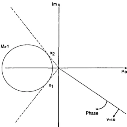
Figure 3.3: M circle for M

> 1

3.1.3 Transfer of

M

circles to Nichols Plot

Based on the value of M, the pattern of the M circles on the Nichols chart can be obtained for the three cases outlined in the previous section. To transfer the M circles to the Nichols chart, consider a straight line (constant phase) through the origin described by the equation

v = lu (3.8)

where u and v denote the real and imaginary parts of the open-loop frequency response respectively. To transfer the M-circles to the Nichols chart we need to solve the two equations (AI-circle and straight line) simultaneously.

Case 1

When M

> 1 the circle will lie to the left or the negative half of the Nyquist plot as

shown in figure 3.3.

From figure 3.3 it can be noticed that as the fixed phase line rotates through 360° it can be the tangent of the circle on two occasions, at point Xl and X:!. Thus the M circle on the Nichols plot will be defined only for the phase range:

[image:37.549.167.376.46.254.2]

30

20 CD

~ 10

c -iii o

0. 0 r:'"~""""'_ o

o

...J

C:

~ -10

o

-20

-30

-350

Re

Figure 3.4: M circle when M = 1

, .

, ,

--300 -250 -200 -150 -100 -50

Open~ccp Phase (deg)

o

Figure 3.5: M circle on Nichols Plot for M

>

1, M

<

1, M = 1

[image:38.552.89.505.51.790.2] [image:38.552.153.385.58.366.2]

1m

Phase

Re

Figure 3.6: M circle when M

<

1

For any 4> (strictly) inside this interval there are exactly two (positive) solutions to the system of simultaneous equations corresponding to the M - circle and the straight line. It follows that the M circle on the Nichols chart in this case is a closed contour as shown in the figure 3.5.

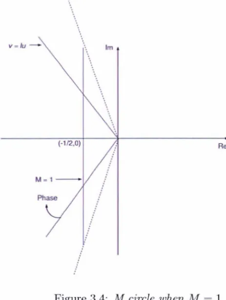
Case 2

As shown in figure 3.4 the M circle is a vertical line through the point (-~, 0). Thus the closed-loop magnitude will tend to infinity when the open-loop phase approaches -2700 _{and -90}0

• Clearly, in this case the simultaneous equations have one positive

and one negative solution, the later being discarded since it cannot represent a gain variable. Converting this plot to Nichols chart corresponds to an open contour defined for phases in the open interval - 2700 _{to -90}0 _{only and tending to infinity as we}

ap-proach these two phases.

Case 3

20

J-~---~~~---~-~ ,

, , , ,

__ J'\

Plhlft IVIargi"

- ' , - ' - - - ' ~~----­ ,

,

tt

2

dB ,

" ,

Opm-lccp Phase deg)

Figure 3.7: Nichols Plot

the straight line we always get two distinct positive solutions for Xl and 1i.l, i.e. Xl =I- 1i.l.

Thus the plot of M -circles on the Nichols chart will be an open-ended contour as shown

in the figure 3 ..

For an open-loop stable system G(s), the maximum magnitude ratio Mp is obtained

by finding the largest M contour which touches, but does not cross the G(jw) locus.

Mp is a useful design parameter since it indicates the maximum (''resonance'') peak of

the closed-loop magnitude frequency response, or indirectly the "minimum damping"

of the system. The frequency corresponding to Mp wp say, is not a direct reading,

but can be easy obtained by interpolating the frequency-response G(jw) data points.

The bandwidth of the closed-loop system is similarly found from the intersection of

the G(jw) locus with the -3dB contour. Since all M - circles on the Nyquist plane

are symmetric with respect to the negative real axis the corresponding contours in the

Nichols chart will be symmetric relative to the 1>

= -180° line.

3.2

Stability

A stable system is an absolute requirement for any control design. The system's sta-bility conditions can be different in its open-loop and closed-loop state, and thus an open-loop stable system does not necessarily imply a closed-loop stable system. There are various methods available to check system stability. The most direct method is to identify the location of the closed-loop poles, which must all lie in the open left-half of the complex plane (i.e. have negative real parts). However, this test requirs the full knowledge of the plant model and does not generalise easily to a test for "robust" stability, since this would typically require the calculation of the poles of an infinite number of systems (each corresponding to an uncertain plant). The most versatile sta-bility test is based on the Nyquist stasta-bility criterion. This requires only the frequency response of the open-loop system (and the number of open-loop unstable poles) and generalises easily to produce robust-stability tests.

As mentioned earlier the QFT problem is traditionally formulated using the Nichols chart. Thus, in this section, the Nyquist stability criterion is re-formulated in this domain.

3.2.1 Nyquist Stability Criterion

The Nyquist stability criterion relates the total number of encirclements of the open-loop frequency response around the critical (-1) point to the number of the system's closed-loop poles that lie in the right half of the s - plane. The Nyquist stability crite-rion is based on the result from complex analysis, known in the literature as Cauchy's principle of the argument.

[23, 8].

1m

Figure 3.8: S - Plane

The coefficient A-I is called the residue of G(s) at So and may be evaluated as

A-I

=

Res[G(s); So]

=

~

1

G(s)ds

271"

Ie

(3.10)

where c denotes a closed arc within an analytic region centered at So that contains no other singularities.

Theorem: Let G(s) be an analytic function inside and on a closed contour C except for a finite number of poles inside C. Then, as we transverse C in the clockwise direction,

Equivalently:

~

f

G' (s) ds = Z - P

271" G(s)

~

f

d (InG) = Z - P 271"

where Z is the number of zeros and P is the number of poles inside C.

(3.11)

Proof:- Let So be a zero of G with multiplicity k. Then in some neighbourhood of that point we may write G(s) as:

where f(s) is analytic and f(so)

=I

O. If we differentiate equation 3.9, we get

G'(s) = k(s - so)k-l f(s)

+

(s - so)k I'(s)

from which it follows that:

G'(s) k I'(s) G(s) - s - So

+

f(s)

Therefore C;;(~l has a pole s = So with residue k. This procedure is repeated for every zero. Hence the sum of the residues of

C;;gl

is the number of zeros of G(s) inside C. If

So is a pole with multiplicity 1, we may write G( s) as

where h(s) is an analytic function and h(s)

=I

O. From equation 3.13 we get:

G(s) = h(s) (s - so)1

Differentiating the above equation gives:

so that

G'(s)

=

h'(s) Ih(s) (s - so)1 (s - so)l+!

G'(s) G(s)

-1 h'(s)

- - + - -

_{s - So h(s)}

(3.13)

This analysis is repeated for very pole. It follows that the sum of the residues of

C;;(W

at every pole of G(s) is equal to -Po Using equation 3.10

-21.

i

d(1nG(s)) = Z - P

71] c

where d(lnG(s)) was substituted for C;;(~1 ds. If we write G(s) in polar form then

i

d(lnG(s)) =

i

d (InIG(s)1

+

j arg(lnG(s))

- I IG( ) 118

=82 • G() 18=82

- n s 8=81

+

Jarg s 8=81

Since

r

is a closed contour, the first term is zero, and the second term is S7r times the net encirclements of the origin. Thus:

as required.

~

J

d(lnG(s)) = Z - P

27rJ

1'r

28

Remark: If G(s) is stable, then its unity feedback closed-loop system is also stable if and only if, the Nyquist contour does not encircle the (-1,0) point. If G( s) has P poles in the right-half of the s-plane, then the number of counter-clockwise encirclements of the (-1,0) point must be equal to P for the corresponding closed-loop system to be stable. [58].

3.2.2 Stability criterion on the Nichols Chart

Since QFT design is carried out on the Nichols plane, it is sensible to have a criterion to specify stability of a system directly in this plane. A version of Nyquist stability cri-terion on the Nichols chart was first developed in [43]; this was further improved in [12].

The stability criterion on the Nichols chart is a re-formulation of the Nyquist stabil-ity criterion. Stabilstabil-ity of a system in the Nyquist plane is mainly based in the Zero

exclusion theorem, i.e. for a system to be stable the condition 1

+

L(jw)

=I

°

should hold, and the net encirclements of the critical point -1 should be zero i.e. N = P - Z where P is the number of poles and Z is the number of zeros of the system. In the Nyquist plot the direction of the system response produced by an unstable pole is in the anti-clockwise direction in the left half of the Nyquist - plane and this is called Negative crossing of the stability line Se. The response produced by a zero in the system is in the clock-wise direction in the left half of the Nyquist - plane, and this is called Positive crossing of the stability line Be. The stability line together with typical positive and negative crossings are shown in the figure 3.9.

Firstly the stability line Se which contains the critical point -1 in the Nyquist plane is translated onto the Nichols chart. The stability line in the Nyquist plane is given by

Se =: {(x,y): y = O,x

< -I}

(3.14)

Se is translated onto the Nichols chart using the relations Z

=

a

+

ib, where a

=

r cos () and b = r sin () (in this case a = -1 and b = 0), and so the stability line on the Nichols chart Sn is given by

1m

/

...

---Nyquist Plane

.Sn ~

~-+n

i

Stability Lin Od - - -

--180°

Nichols Chart

Figure 3.9: Positive and Negative crossing, and stability lines Se and Sn on the Nyquist plane and Nichols chart

The stability lines on the yquist plane and on the Nichols chart are shown in figure

3.9. The stability criterion on the Nichols chart is formulated by applying the Nyquist

stability criterion on the Nichols chart. The stability line in the Nichols chart is given

by Sn, this line corresponds to the stability line Se in the Nyquist chart as shown in

figure 3.9. The stability analysis of a plant in the Nichols chart is based on the number

of positive and negative crossing's of the stability line Sn by the open-loop response of

the system.

To introduce the stability condition a stable system with n stable poles in equation

3.16 is considered. Let:

L( ) _s = N(s) _D(s) (3.16)

The poles of the above system lie in the left half of the s - plane. The closed-loop

stability of the syst m for various cases is guaranteed by the conditions below:

• For a system whose response lies above the line r = 0 dB the open-loop response

should pass through the line r = 0 dB, in the range -180°

<

180° to make the

system response stable.

• As a direct consequence of the yquist stability criterion, the net positive

and negative crossings of the stability line RL = : ¢ = -180°, r = [0, (0) and RL =: ¢ = 1 0°, r = [0,(0), hould be zero, i.e. if the system response crosses

the stability lines RL or RR then, in order for the system to be stable, the

. J - _ -_ _ .A

OdB

o

-180

Fig a

dB's

OdB

rad's

Fig b

Figure 3.10: Stability region shown on Nichols chari, Fig (a) A. One crossing B. No corssing, Fig (b) Several crossings

response should re-enter the stability region. Then the response should cross the line r

=

OdB within the stability lines, thus satisfying the above condition. • For a plant whose open-loop response starts below the line r = OdB, the system

is always stable.

Nichols stability criterion for Unstable/Non minimum phase plants

The region of the open-loop response plot on the Nichols chart will be dictated by the presence of an unstable pole or zero in the plant. Depending on the number of unstable poles or poles the system response is shifted towards the right in multiples of n, where n is the pole-zero excess of the system. The stability of a system is checked

using Nichols stability criterion by first transforming the unstable/non-minimum phase plant into a stable/minimum-phase plant, then shifting the robust stability bounds by a specific amount in the horizontal axis (phase value), and finally applying the stability criterion. In the process of converting the unstable/non-minimum phase plant into a stable/minimum-phase plant, the gain of the plant response should not be altered, in order to retain the plant characteristics. A procedure for finding the required phase shift for the robust bounds is given in [13, 25]. First consider an unstable/non

phase system factored as:

PN(S) =

N(s)~(

-S)

D(s)P( -S) (3.17)

where

Z (

-s) is an unstable polynomial containing all the non-minimum phase zeros of N(s), i.e. all zeros in the right half of the s - plane; similarly P( -s) contains all unstable poles, i.e. all plant poles in the right half of the s- plane. The general expression for robust stability margin for a plant in QFT design is given by:

(3.18)

where LN(S) = PN(s)KN(S) and 'Y is a constant. Here PN(S) denotes the transfer function of the plant and KN(S) the transfer function of the feedback controller. The subscript N is used to avoid confusion with previous sections, and emphasises that the discussion here is based on the Nichols chart. Let the nominal plant for this system be given by:

(3.19)

In order to achieve a stable/minimum phase system, without affecting the magnitude frequency response of PNJs), while shifting its phase response along the horizontal axis, define:

(3.20) Clearly A(s) is an all-pass function, i.e. IA(jw)1 = 1 for all wE [0,00). Define also:

P,vJs)

= PNJs)A-l(S)

No(s)Zo(s)

-Do(s)Po(s)

and note that the system in equation 3.22 is stable and minimum-phase. Now,

(3.21)

(3.22)

where L',y(s) = Pfv(s)KN(s) and Pfv(s) = PN(s)A-l(S). Then, for a general frequency

w,

the robust stability condition is given by:

I

LN(jW)

I-I

L',y(jw)

I

<

1

+

LN(jW) - A(jw)

+

L',y(jw) - "Y (3.23)

Since LN(jW)

=

:NVw\LNJjw), the robust stability condition in equation 3.23 for a

No JW

nominal plant is given by:

(3.24)