Algorithmic issues for three-invariant hyperplastic Critical State models

      

City, University of London Institutional Repository

Citation

:

Coombs, W.M. and Crouch, R.S. (2011). Algorithmic issues for three-invariant

hyperplastic Critical State models. Computer Methods in Applied Mechanics and

Engineering, 200(25-28), pp. 2297-2318. doi: 10.1016/j.cma.2011.03.019

This is the accepted version of the paper.

This version of the publication may differ from the final published

version.

Permanent repository link:

http://openaccess.city.ac.uk/15546/

Link to published version

:

http://dx.doi.org/10.1016/j.cma.2011.03.019

Copyright and reuse:

City Research Online aims to make research

outputs of City, University of London available to a wider audience.

Copyright and Moral Rights remain with the author(s) and/or copyright

holders. URLs from City Research Online may be freely distributed and

linked to.

Algorithmic issues for three-invariant hyperplastic Critical State models

William M. Coombs, Roger S. Crouch

⇑

Durham University, School of Engineering and Computing Sciences, South Road, Durham DH1 3LE, United Kingdom

a b s t r a c t

Implicit stress integration and the consistent tangents are presented for Critical State hyperplasticity models which include a dependence on the third invariant of stress. An elliptical deviatoric yielding cri-terion[43]is incorporated within the family of geotechnical models first proposed by Collins and Hilder

[8]. An alternative expression for the yield function is proposed and the consequences of different forms of that function are revealed in terms of the stability and efficiency of the stress return algorithm. Errors associated with the integration scheme are presented. It is shown how calibration of the two new mate-rial constants is achieved through examining one-dimesional consolidation tests and undrained triaxial compression data. Material point simulations of drained triaxial compression tests are then compared with established experimental results. Strain probe analyses are used to demonstrate the concepts of energy dissipation and stored plastic work along with the robustness of the integration method. Over twenty finite element boundary value problems are then simulated. These include single three-dimensional element tests, plane strain footing analyses and cavity expansion tests. The rapid convergence of the global Newton–Raphson procedure using the consistent tangent is demonstrated in small strain and finite deformation simulations.

1. Introduction

Following on from the pioneering work of Ziegler[45], Houlsby

[26]and Collins and Houlsby[6], a number of constitutive models based on a hyperplasticity framework have been constructed for geomaterials[7–14,28,29,35,36]. These offer improvements over conventional plasticity formulations which can fail to satisfy fun-damental thermodynamic principles. Hyperplasticity establishes the constitutive model using just two scalar functions; the free-en-ergy function and the dissipation function. Curiously, despite their attraction, very few hyperplasticity models have been incorporated and tested in generalised numerical analysis schemes such as the finite element method. In particular, to date, the consistent linear-isation (stress integration and algorithmic tangent) for the isotro-pic family of non-linearly hardening constitutive models proposed by Collins and Hilder[8](further developed by Collins et al.[9–11,13]) has yet to be presented. These formulations em-brace the condition, known as the Critical State[38], whereby un-bounded plastic distortions take place with no change in state (constant stress and volume). Here we provide the linearisation and illustrate the performance of these extended models using both material point and boundary value simulations. The work will be of particular interest to those simulating the compactive-dilative inelastic response of granular material.

The paper is organised as follows. Section2presents the consti-tutive formulation, including (i) the hyperelastic relationship, (ii) the plasticity relations, (iii) the introduction of the Willam–Warn-ke (W–W) [43]Lode angle dependency (LAD) within the hyper-plastic framework and (iv) calibration of the non-classical material parameters. Here we make use of a different means of introducing a LAD (compared to Collins and Hilder[8]) in order to overcome previous limitations. Application of the backward Eu-ler (BE) stress integration for these models is thoroughly described in Section3together with an assessment of the magnitude of the errors associated with the stress return. Derivation of the consis-tent algorithmic tangent is presented in Section4. Numerical sim-ulations are reported in Section5for material point tests and for over twenty finite element simulations (i) a simple single 3D ele-ment test (ii) numerical verification through a plane strain flexible footing comparison with Borja and Tamagnini [3] (iii) a plane strain smooth rigid footing problem and (iv) finite deformation cylindrical cavity expansion.

The majority of the relations given in this paper are expressed using principal stresses. In all that follows {} and [] denote 3 by 1 vectors and 3 by 3 matrices, respectively and {}Tdenotes a vector transpose.f^g and½^are used to indicate six-component vectors and matrices respectively. We use the standard notation where (),xand (),xxexpress the first and second derivatives of () with

All stresses are treated as effective stresses although the standard prime notation will be omitted. For compactness, Section2, adopts tensor subscript notation whereas Sections2.1onwards use matrix and vector notation.

2. Hyperplastic constitutive formulation

The fundamental assumption for hyperplastic formulations is that the constitutive equations can be derived from a free-energy function and a dissipation function. Once these have been speci-fied, the stress–elastic strain law, yield function and flow rule can all be obtained without the requirement for any additional assumptions. Textbook accounts of the thermomechanics of mate-rials can be found in the volumes by Ziegler[45]and Maugin[33], amongst others. The following introduction (up to Section 2.1) draws heavily from the work of Collins et al.[6–14]. The rate of work done per unit volume is given by

r

ij

e

_ij¼

W

_ þ

U

_; ð1Þ

whereWdenotes the free-energy function and_U_ _{identifies the}

dis-sipation rate. Both the free-energy function and disdis-sipation rate are defined per unit volume.

rij

represents the stress tensor and

e

_ijthe

total strain rate tensor.

The free energy function is typically defined in terms of the to-tal,

eij

, and plastic,

e

p

ij, strains[6]. However, here we limit ourselves

to the case of de-coupled materials whereW (and its associated rate) can be split into two components: one in terms of the elastic strains and the other in terms of the plastic strains

W

¼

W

1ð

e

eijÞ þ

W

2ð

e

pijÞ and

W

_ ¼

@

W

1

@

e

e

ij !

_

e

e

ijþ

@

W

2

@

e

p_ij

!

_

e

p

ij: ð2Þ

The first term gives the true stresses in terms of the elastic strains

r

ij¼

@

W

1

@

e

e

ij

; ð3Þ

whereas the second term in(2)2provides theshift stress

v

ij¼

@

W

2

@

e

p

ij

: ð4Þ

This identifies thecentreof the yield surface in true stress space. Through these shift stresses, the second component of the free-energy function describes the kinematic hardening of the yield sur-face. Isotropic hardening is controlled by the dissipation rate. That rate depends on the plastic strain rate in addition to the total strains,_U__ð

_e

ij;

e

pij;

e

_ p

ijÞ. It cannot depend on the total strain rate,

other-wise purely elastic deformation would result in dissipation. For

inviscid elasto-plasticity models, the dissipation rate is homoge-neous of degree one in the plastic strain rates[7], giving

_

U

¼@ð

U

_Þ

@ð

_e

_p

ijÞ

_

e

p

ij: ð5Þ

For frictional materials the dissipation rate depends on the total volumetric strain (or the effective pressure) but(5) remains un-changed. Using the dissipation rate we can define adissipative stress space

u

ij¼

@ð

U

_Þ

@ð

_e

_p

ijÞ

; ð6Þ

thus(5)becomes

_

U

¼

u

ij

e

_

p

ij: ð7Þ

The dissipative stress is linked to true stress through the shift stress,

v

ij. Substituting(2)2and (7)into(1), we obtain

r

ij

e

_ij¼

@

W

1

@

e

e

ij

_

e

e

ijþ

@

W

2

@

e

p_ij

e

_

p

ij !

þ

u

ij

e

_

p

ij: ð8Þ

Using(3) and (4), (8)becomes

r

ij

e

_ij¼

r

ij

e

_eijþ

v

ijþ

u

ij

_

e

p

ij; ð9Þ

which, due to the additive decomposition of the strain rate

eij

¼

e

e ijþ

e

p

ij, provides the following relationship between total, shift

and dissipative stresses

r

ij¼

v

ijþ

u

ij: ð10Þ

The dissipation rate is not equal to the plastic work rate. The latter is given by the product of the true stress with plastic strain rate

_

Wp_¼

_r

ij

e

_pij¼

U

_ þ

v

ij

e

_

p

ij: ð11Þ

Due to the constraints imposed by the second law of thermodynam-ics,_U_ _{must always be greater or equal to zero, but there is no}

restriction on the sign of_W_p_{. The last term in (11)indicates the}

plastic work associated with the recoverable elastic deformations arising from plastic strains when grains arelockedin position within the material fabric[12]. The concepts of dissipated and stored plas-tic work can be appreciated using the one-dimensional kinemati-cally hardening model in Fig. 1(i). This rheological analogue comprises a spring (a) which is in parallel with a second spring and slider (b). In the example plot, the system is subjected to an increasing total stress,

r

, followed by unloading until

rb

= 0;

[image:3.595.54.537.588.733.2]

Fig. 1(ii). The components of stored and dissipated plastic work

can be seen inFig. 1(iii). Plastic dissipation occurs in the slider. Stored plastic work is a consequence of the frozen elastic energy in spring (a) which is restrained by the plastic slider.

It can be shown that the plastic strain increment is given by a normal flow rule indissipative stress space[6]. This only implies an associated model intrue stress spaceunder the condition that the dissipation rate is independent of the true stress,

rij

. For this case, when the free-energy function only depends on the elastic strains, the shift stresses are zero and the true and dissipative stress spaces are identical.

2.1. Hyperelastic relationship

Particulate geomaterials typically demonstrate a dependence of the elastic bulk modulus on the current effective pressure, or equivalently on the current elastic volumetric strain. One common approach[21]is to specify the elastic shear modulus directly from the bulk modulus assuming a constant Poisson’s ratio. However, this leads to a non-linear elasticity model in which energy can be generated from certain loading cycles[3,27,46]. Here we use a var-iable bulk modulus with a constant shear modulus[27]. This can be realised by adopting an elastic free-energy function of the form

W

1¼

jp

rexp

e

e

v

e

ev0

j

þG _{f g}

c

e T

c

e

f g

with

e

e

v¼tr½

e

e andf g ¼

c

e f g

e

e

e

e

v 3f1g

; ð12Þ

where

j

is the elastic compressibility index,Gis the shear modulus,

pris the reference pressure,

e

ev0is the elastic volumetric strain at

that reference pressure and {1} = {1 1 1}T. The true stress is given by the first derivative of(12)with respect to elastic strain

r

f g ¼f

W

1;eeg ¼p_rexp

e

e

v

e

ev0

j

f1g þ2Gf

c

e_{g: ð13Þ}

The principal non-linear elastic stiffness matrix is obtained from the second derivative of(12)with respect to elastic strain

½De ¼ ½

W

1;ee_ee ¼ K2G

3

f1gf1gTþ2G½I;

whereK¼pr

j

exp

e

e

v

e

ev0

j

ð14Þ

and [I] is the third order identity matrix. The six-component elastic compliance matrix is giving by

b

Ce

h i

¼hDbei1_¼ C e

½0

½0 G1

½I

" #

where½Ce ¼1 9 1 K 3G 2

f1gf1gTþ 1

2G½I ð15Þ

and [0] is the 3 by 3 null matrix.

2.2. Plasticity relations

As proposed by Collins and Hilder[8], atwo-parameterfamily of Critical State[38]models can be defined using the following dissi-pation function _

U

¼ ffiffiffiffiffiffiffiffiffiffiffiffiffiffiffiffiffiffiffiffiffiffiffiffiffiffiffiffiffiffiffiffiffi _

e

p vA ð Þ2þ

e

_p

cB

2

q

; where

A¼ ð1

c

Þpþ

c

2pc andB¼M ð1

a

Þpþ

ac

2 pc

: ð16Þ

The weight parameters

a

,

c

2[0, 1] influence the shape of the yield surface (as shown inFig. 2)and the degree of non-association of the plastic flow direction.p= tr ([

r

])/3 is the mean pressure andpc

de-fines the size of the yield surface.Mis the stress ratio at which con-stant volume plastic shearing occurs (geometrically, this is the gradient of the Critical State line inp–qspace, seeFig. 3(i)). The plastic strain invariants are defined as follows

e

p

v¼tr½

e

p and

e

pc¼

ffiffiffiffiffiffiffiffiffiffiffiffiffiffiffiffiffiffiffiffiffiffi

f

c

p_gT f

c

p_g

q

; withf

c

p_{g ¼ f}

_e

p_g

e

p

v 3f1g:

ð17Þ

The deviatoric stress invariant,q, is similarly given by

q¼

ffiffiffiffiffiffiffiffiffiffiffiffiffiffiffiffi

fsgTfsg

q

; withfsg ¼ f

r

g pf1g: ð18Þ

Note that thisq(18)1differs from that often used when describing

the triaxial tests of soils (there q= (

r3

r1

)). Assuming a free-energy function of the form[6]

W

¼

W

1ðf

e

egÞ þ

W

2ðf

e

pgÞ;

W

2ðf

e

pgÞ ¼

c

ðk

j

Þ 2 prexp

e

p

v

k

j

;

ð19Þ

withW1given by(12), we can define the shift stress as

f

v

g ¼

cp

c

2 f1g; withpc¼prexp

e

p

v

k

j

: ð20Þ

[image:4.595.98.517.571.741.2]

Moving between dissipative and true stress space corresponds to a (pressure dependent) hydrostatic shifting of the yield surface. The

form of hardening implied by(19) and (20)gives rise to an isotropic expansion/contraction of the surface coupled with a (kinematic) translation along the hydrostatic axis, as shown in Fig. 3(i). We can now define the dissipative stress invariants as

pu¼@

U

_

@

_e

_p

v¼ A2

e

_p

v

_

U

andq

u_¼@

U

_

@

_e

_p

c ¼B 2_{_}

e

p c _

U

: ð21Þ

Rearranging, we obtain the plastic strain rates as

_

e

p

v¼ pu

_U

_

A2 and

e

_

p

c¼

qu

_U

_

B2 : ð22Þ

Substituting(22)into(16)and eliminating_U__{, we obtain the}

dissipa-tive yield condition

fu¼ ðpuÞ2B2þ ðquÞ2A2A2B2¼0: ð23Þ

This defines an ellipse in dissipative (pu,qu) stress space. The dissi-pative stress invariantspuandquare given by

pu_¼1

3tr½

u

andq

u_¼ ffiffiffiffiffiffiffiffiffiffiffiffiffiffiffiffiffiffiffiffiffiffi_fsu_gT fsu_g q

; wherefsu_{g ¼ f}

_u

_{g p}u_f1g:

ð24Þ

By substituting (p–pv) forpuandqforqu, we arrive at the following expression for the yield function in true stress space

f¼ ðp

cp

c=2Þ

2_B2

þq2_A2

A2_B2

¼0: ð25Þ

For this f the Critical State Surface (CSS) takes the form of a Drucker–Prager circular cone. If

a

=

c

= 1, thenA=B=pc/2 and we

recover the conventional modified Cam–Clay (MCC) yield function with associated plastic flow[37]. In this case, moving between dis-sipative and true stress space involves a constant hydrostatic trans-lation of the yield surface, asAandBare only dependent onpc. For

values of

c

2[0, 1], the intersection of the CSS and the yield surface occurs atp=

c

pc/2. The value of

a

has no influence on that location.

As

c

reduces, the yield surface becomes narrower deviatorically (see

Fig. 2(ii)). When

c

= 0, the yield surface radius disappears. As

a

re-duces, so the yield surface becomes more tear-drop shaped (with the tail at the stress origin); seeFig. 2. For

a

< 0.172 the yield surface becomes concave near the stress origin (Fig. 2)[9]. When

a

= 0 the yield surface lies entirely within the CSS.

Through the following simplification of(25), the yield function can be written as

f¼ ðp

c

pc=2Þ 2

A2

B2þA2q2

;

¼ p2

_c

_p

cpþ

c

2ðpcÞ 2

=4 ð1

c

Þ2p2

_c

_ð1

_c

_Þp

cp

c

2ðpcÞ 2

=4

B2þA2q2

;

¼

c

ð2

c

Þp2

_c

_ð2

_c

_Þp cp

B2_þA2_q2

;

¼

c

pð2

c

ÞðppcÞB

2_þA2_q2_¼0

: ð26Þ

For this family of hyperplastic models, the direction of plastic flow is normal to the yield surface indissipative stress space. Thus the dis-sipative plastic flow direction is formed by taking the derivative of

(23)with respect to the dissipative stress

ffu_;

ug ¼ fu;pufpu;_ug þ fu;qufqu;_ug: ð27Þ

Using(24), (27)becomes

ffu_; ug ¼

2 3B

2_pu_{f1g þ2A}2

fsu_{g: ð28Þ}

Transforming into true stress space we obtain the direction of plas-tic flow as

fg;rg ¼ 2 3B

2

ðp

cp

c=2Þf1g þ2A

2

fsg; ð29Þ

where the notation {g,r} is used to suggest an equivalence with the

derivative of the plastic potential used in conventional non-associated plasticity.Fig. 4shows the direction of plastic flow for the two-parameter model with (i)

a

= 0.5 and

c

= 1 and (ii)

a

= 1 and

c

= 0.5.

Using(16) and (19)2we have obtained the yield surface,

direc-tion of plastic flow and the isotropic hardening equadirec-tions, along with the hyperelastic relationship from (12), to fully define the constitutive relationship.

2.3. Lode angle dependency

The Lode angle is given by

h¼1 3arcsin

3pffiffiffi3 2

J3

ðJ2Þ 3=2

!

2 ½

p

=6;

p

=6; ð30Þ

where the invariantsJ2andJ3are defined by J2¼ s21þs22þs23

=2 andJ3¼ s31þs32þs33

=3, respectively. It has been shown that ignor-ing the dependence of constitutive relations on the third invariant of stress can lead to significant overestimation of the stiffness in geotechnical analyses[15,18,34]. A number of Lode angle depen-dencies have been proposed in the literature, for example

[1,2,31,32,39,43]. Collins[9]combined the Matsuoka–Nakai yield condition with the Critical State cone by redefiningqin the Spatially Mobilised Plane (SMP)[32]. However, implementing the Matsuoka– Nakai deviatoric yielding criteria in this manner constrains the prin-cipal admissible stress states to be compressive[8]. This can result in instabilities when constructing an implicit stress return algo-rithm where trial points lie in the tensile region.

Here we follow an alternative approach by introducing the LAD into the constitutive equations as follows

[image:5.595.86.503.65.220.2]

Bh¼

q

ðhÞB; ð31Þ

whereBis given by(A.1)3.

q

ðhÞ ¼

q

ðhÞ=

q

cis the normalised

devia-toric radius and

qc

is the deviatoric radius required to reach yield under a triaxial compression stress path where

r3

/2 =

r2

=

r1

.

Fig. 5compares Lode angle functions from[1,43,32,2](with a

nor-malised shear radius

qs

¼0:73 on the shear meridian) and [39]

for

qe

¼0:656.

qe

is the ratio of the deviatoric radius at yield under triaxial extension to the deviatoric radius (at the same mean stress) under triaxial compression. The multiaxial experimental data[31]

shown in the figure indicate that geomaterials can have both a LAD (Fig. 5(i)) and a sensitivity to the intermediate principal stress (Fig. 5(ii)). The effective friction angle inFig. 5(ii) is calculated from the expression given by Griffiths[23]

/¼arcsin

ffiffiffi

3 p

gcos

ðhÞ

ffiffiffi

2 p

þ

g

sinðhÞ

!

; ð32Þ

where

g

¼q=ðpffiffiffi3pÞ. InFig. 5, the M–C envelope (unlike the other deviatoric functions) exhibits no sensitivity to

r2

. The Gudehus LAD significantly overestimates both the normalised deviatoric ra-dius and the effective friction angle. Although the Bhowmik–Long LAD arguably provides the most satisfactory fit to the experimental data, it requires an additional parameter

qs

which can only be cal-ibrated using a multiaxial test apparatus, of which there are very few. The W–W LAD provides a balance between offering good agreement with the experimental data yet requiring only one addi-tional parameter,

qe

.

The W–W LAD (as seen inFig. 6) can be expressed as

q

ðhÞ ¼a1Cþ

ffiffiffiffiffiffiffiffiffiffiffiffiffiffiffiffiffiffiffiffiffiffiffiffi

2a1C2þa2

q

2a1C2þ1

2 ½

q

e;1

wherea1¼

2ð1

q

2

eÞ ð2

_q

_e1Þ2

; a2¼

5

q

2

e4

q

e

[image:6.595.92.516.67.201.2]

ð2

_q

_e1Þ2 ð33Þ

[image:6.595.93.518.233.413.2]

Fig. 4.Yield surfaces and direction of plastic flow for the two-parameter Critical State models: (i)a= 0.5 andc= 1 (ii)a= 1 andc= 0.5.

Fig. 5.Comparison of Lode angle deviatoric functions with experimental data from Lade and Duncan[31](i) deviatoric function Lode angle dependency and (ii) variation of the effective friction angle with the ratio of the intermediate principal stress.

[image:6.595.62.273.459.666.2]

andC= cos (h+

p

/6). This describes a deviatoric section (with six-fold symmetry) formed by a portion of an ellipse. In the absence of triaxial extension data, we can estimate

qe

based on the friction angle (/) through

q

e¼

2þk

2kþ1; wherek¼

1þsinð/Þ

1sinð/Þ; ð34Þ

so that

qe

coincides with that of Mohr–Coulomb. The gradientM

when h=

p

/6 is obtained (again from the friction angle) through the rearrangement of(32)

M¼2

ffiffiffi

6 p

sinð/Þ

3sinð/Þ: ð35Þ

For other Lode angles, the gradient is given by

q

ðhÞM. Note the non-standard definition ofMbased on the friction angle due to the def-inition ofqfrom(18)1, resulting in a difference of

ffiffiffiffiffiffiffiffi

2=3

p

between

(35)and the standard definition. The yield equation and the direc-tion of plastic flow are now expressed as

f¼ð

cp

ð2

c

ÞðppcÞÞðBhÞ

2

þA2q2

¼0; and

fg;rg ¼ 2 3ðBhÞ

2

ðp

cp

c=2Þf1g þ2A

2

fsg: ð36Þ

The effect of introducing a W–W LAD on the different members of the family of constitutive models can be seen inFig. 7. The three

yield surfaces correspond to (i)

a

=

c

= 1, (ii)

a

= 0.5,

c

= 1 and (iii)

a

= 1,

c

= 0.5 with

qe

¼0:8 and a friction angle of/=

p

/9 radians.

2.4. Calibration of

a

and

c

The two material constants,

a

and

c

, which extend the classical MCC model may be determined from examining undrained triaxial and one-dimensional consolidation data. In this calibration proce-dure we assume that, under sufficiently large straining during one-dimensional consolidation, the elastic strains are negligible. In this case the ratio of the deviatoric to volumetric plastic strains is

_

e

p

c

_

e

p

v¼

A2ð

g

K0Þ

B2 ₁

c

ðpc=pÞ=2

ð Þ¼

ffiffiffi

2 3

r

; ð37Þ

where

g

K0¼q=pis the stress ratio under one-dimensional (K0)

con-solidation. Substituting(26)forB2and rearranging, we obtain the ratio of the size of the yield surface to the pressure as

pc

p ¼

c

ð2

c

Þ þ ð

g

K0Þ

ffiffiffiffiffiffiffiffi

2=3

p

c

ð2

c

Þ þ

c

ð

g

K0Þ

ffiffiffiffiffiffiffiffi

1=6

p : ð38Þ

From(26),

a

can then be obtained as

a

¼

g

K0

1þ

c

½ðpc=pÞ=21

ð Þð

c

ð2

c

Þ ð½ pc=pÞ 1Þ 1=2

M Mð

c

ðpc=pÞ=21Þ

:

[image:7.595.78.534.347.479.2]

ð39Þ

Fig. 7.Two-parameter Critical State family of models with W–W deviatoric sections: (i)a=c= 1, (ii)a= 0.5,c= 1 and (iii)a= 1,c= 0.5.

[image:7.595.80.505.516.724.2]

However,(39)and(38)require the specification of

c

which can be determined from undrained triaxial compression (UTC) or exten-sion data at an overconsolidation ratio (OCR) of two. Fig. 8 (ii) shows UTC test results from Gens[20]. For OCR = 2, the change of normalised pressure between the starting and final stress states can be used to approximate

c

, as shown inFig. 8(ii), as

c

pf pi

¼2pf pc

; ð40Þ

wherepi=pc/2 andpfare the initial and final stress states from the

UTC experiment. The change in the size of the yield surface will be small due to the near isochoric plastic flow (being in close proxim-ity with the Critical State) such that 2pf/pc offers a reasonable

approximation for

c

.

In the absence of one-dimensional consolidation data, Jaky’s

[30]formula may be used to approximate the stress ratio under

K0loading

g

K0¼

ffiffiffi

6 p

sinð/Þ

32 sinð/Þ; ð41Þ

where/is the effective friction angle.Fig. 9(i) compares the exper-imental data collated by Federico et al.[19]with(41). Jaky’s for-mula provides an adequate approximation to the experimental data, capturing the general trend. The value of

a

to achieve theK0

consolidation stress ratio

g

_K

0 for

c

= 0.8, 0.9 and 1.0 is given in Fig. 9(ii) for both the experimental data collated by Federico et al.

[19]and for Jaky’s formula. For a friction angle of 25°, Jaky’s formula predicts a stress ratio of

g

_K

[image:8.595.142.463.242.724.2]

0¼0:480 which is achievable with

a

= 0.336, 0.246, 0.175 for

c

= 1.0, 0.9 and 0.8, respectively.

Fig. 9.Calibration of material constanta: (i) one-dimensional consolidation stress ratio against friction angle, comparing experimental data (discrete points)[19]against Jaky’s equation[30]and (ii)aranges forc= 0.8, 0.9 and 1.0, corresponding to the data obtained from[19]. Graph (ii) also shows theaversus friciton angle relationships for

Fig. 8(i) compares theK0consolidation data on Lower Cromer

Till (LCT)[20]with the MCC model and the two-parameter model. The experimental data achieves a stress ratio of

g

K0¼0:6, from Fig. 8(ii)

c

0.9 and M= 0.964 (/= 29.5°). Using (38) and (39), we obtain

a

= 0.3. The two-parameter model with

a

= 0.3,

c

= 0.9 provides an excellent fit to the K0 experimental data. For the

MCC model, once the gradient of the Critical State line has been specified, the stress path under one-dimensional consolidation is fixed (that is, K0 is directly dependent upon M). In Fig. 8(i) we

see that the MCC model is not able to provide a good simulation of the K0 consolidation stress path.Fig. 8(ii) compares the UTC

experimental data from Gens [20] with the response from the MCC model and the two-parameter model (

a

= 0.3,

c

= 0.9) for OCR = 2, 4 and 10. The two parameter model provides a significant improvement over the MCC formulation, as the latter significantly overpredicts the stress ratio

g

=q/pprior to arrival at the Critical State.

3. Backward Euler stress integration

Stresses are integrated using the backward Euler scheme which corresponds to the minimisation of

f

r

rg f

r

tg

f gT Ce ff

r

rg f

r

tgg; ð42Þ

with respect to the return stress {

rr

} (see Simo and Hughes[41]). This represents a closest point projection. Within(42), ()tand ()r

denote quantities associated with the trial state and the return state respectively. The minimisation is subject to the following Karush– Kuhn–Tucker conditions

f60;

c

_ P0 andf

c

_ ¼0; ð43Þ

where

c

_is the plastic multiplier (not the deviatoric strain rate or the material parameter first seen in (16)). The popularity of the fully

implicit BE approach over explicit schemes (for example[42]) is due to its relatively high accuracy for a given numerical effort, par-ticularly when large strain increments are applied[5,41].

Working with elastic strains as the primary unknown, we can express the return mapping as

f

e

e

g ¼ f

e

e

tg

Dc

fg;rg; ð44Þ

wheref

e

e

tgis the elastic trial strain (f

e

etg ¼ f

e

eng þ fDeg;nrefers to

the converged state at the end of the previous increment and {De} is the current total strain increment),Dc is the incremental plastic multiplier for the entire return path and the plastic flow direction {g,r} is determined at the final return state. The rate of the evolution

of the size of the yield surface follows from(19)2as

_

pc¼

@pc

@

e

p

v

_

e

p

v¼ pc

k

j

_

e

p

v: ð45Þ

This hardening law is equivalent to specifying a bi-logarithmic lin-ear relationship between specific volume and pre-consolidation pressure[3]. The limitations of the conventional linear relationship between specific volume (or void ratio) and the logarithm of the pre-consolidation pressure were identified by Butterfield[4]. More recently, the appropriateness of the bi-logarithmic law for finite deformation analysis was verified by Hashiguchi[25]and used by Yamakawa et al.[44]. Implicit integration of(45)yields the follow-ing hardenfollow-ing law

~

pc¼

pcn ð1

De

p

v=ðk

j

ÞÞ

; ð46Þ

wherep_cn is the size of the yield surface from the previously con-verged solution associated with the last step (or the initial state at the start of the analysis). We denote the evolution ofpcwith~

to distinguish it from the incremental updating ofpcfrom the BE

[image:9.595.125.465.429.729.2]

method through(61). Using(44) and (46)together with the consis-tency condition,f= 0, we can define the following residuals

fbg ¼ fb1g

b2

b3

8 > < > :

9 > = > ;¼

f

e

e_{g f}

_e

e

tg þ

Dc

fg;rg pc~pc

f

8 > < > :

9 > = > ;¼

f0g 0 0

8 > < > :

9 > = >

;; ð47Þ

with unknowns

fxg ¼ ff x1g x2 x3gT¼ ff

e

eg pc

Dc

g T

: ð48Þ

We obtain the (55) Jacobian matrix from the partial derivatives of the residuals with respect to the unknowns

½A ¼

½A11 fA12g fA13g

fA21gT A22 A23

fA31g

T

A32 A33

2 6 4

3 7 5¼

½b1;x1 fb1;x2g fb1;x3g

fb2;x1g

T

b2;x2 b2;x3

fb3;x1g

T

b3;x2 b3;x3

2 6 6 4

3 7 7 5:

ð49Þ

Forming this matrix, we obtain

½A ¼

½I þ

Dc

½g;rr½De

Dc

fg;rpcg fg;rg fp~c;rgT½De 1 ðp~c;pcÞ ð~pc;DcÞ

ff;rgT½De f;pc 0 2

6 6 4

3 7 7

5; ð50Þ

where [De] is the 33 elastic stiffness matrix(14). The derivatives of~pcare given by

fp~c;rgT¼

Dcp

nf1g T

½g;rr;

ð~pc;pcÞ ¼

Dcp

nfg;rpcg T

f1g; ð~pc;DcÞ ¼pnfg;rgTf1g; ð51Þ

with

pn¼

@~pc

@ð

De

p

vÞ¼

pcn ðk

j

Þð1

De

p

v=ðk

j

ÞÞ2

: ð52Þ

The derivative of the yield function(36)1with respect to the

princi-pal stresses is given by

ff;_rg ¼f;p

3 f1g þ2A

2

fsg þ2c

q

ðhÞB2_p

ð2

c

ÞðppcÞf

q

;rg; ð53Þ

where

f;_p¼ ð2

c

Þ

c

ð2

q

ðhÞMð1

a

ÞðppcÞpþBhð2ppcÞÞBh

þ2Að1

c

Þq2_{: ð54Þ}

The derivativef

q

;rgwill depend on the implemented LAD. Taking the derivative of(33)1with respect toh, we obtain

q

;h¼

a1S bð 1ð1þ2C=b2Þ 4Cða1Cþb2ÞÞ

b21

; where

b1¼2a1C2þ1; b2¼ 2a1C2þa2

1=2

[image:10.595.66.543.67.746.2]

ð55Þ

andS= sin (h+

p

/6). The derivative of

q

(h) with respect to {

r

} is ob-tained through the chain rule as

q

;r¼

q

;hfh;rg; ð56Þ

where the derivative of the Lode angle with respect to stress is gi-ven inAppendix A.1.

Comparing(53)with(36)2 it is apparent that incorporating a

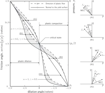
LAD within the constitutive model results in deviatorically non-associated plastic flow (Fig. 6). The model is also volumetrically non-associated (Fig. 4), except for the case

a

=

c

= 1, where the for-mulation reduces to the classical MCC (albeit with a W–W LAD).

Fig. 10 illustrates the variation of the dilation angle (arctanð

e

_p

v=

e

_pcÞ) with the mobilised friction angle (arctan (q/p)). It also shows the direction of the normal to the yield surface, for the case whereM= 1. When

a

= 1 the normals to the yield surface and the direction of plastic flow coincide at q/p=M (arctan (q/

p) =

p

/4), whereas for

a

–1 this is no longer the case. For

a

–1 and

c

–1 {f,r} and {g,r} only coincide at the stress origin and the

compressive closure point on the hydrostatic axis (specifically at

p= 0 andp=pc). When

a

–1 or

c

–1, the normal to the plastic

po-tential is oriented at a lower dilation angle than that given by the normal to the yield surface, for a given stress ratioq/p.

The derivative of(36)1with respect topcis given by

f;pc¼

c

pð2

c

Þð

ca

q

ðhÞMðppcÞ BhÞBhþAq

2

: ð57Þ

From the direction of plastic flow(36)2, the second derivative of

the plastic potential with respect to {

r

} follows as

½g;rr ¼ 1

3fg;rpgf1g T

þ2A2½d þ4 3

q

ðhÞB

2

ðp

cp

c=2Þf1g

f

_q

;rgT; ð58Þ

where [d] = [I]{1}{1}T_{/3 and}

fg;rpg ¼

2 3 B

2

hþ2

q

ðhÞMBhð1

a

Þðp

cp

c=2Þ

f1g þ4Að1

c

Þfsg:

ð59Þ

Finally, the derivative of(36)2with respect topcis obtained as

fg;rpcg ¼

cB

h

3 ð2a

q

ðhÞMðp

cp

c=2Þ BhÞf1g þ2cAfsg: ð60Þ

This provides the derivatives necessary to form(50).

Note that, as a consequence of the magnitude off(with units of stress raised to the power four), it is necessary to dividef, {g,r} and

their associated derivatives by a large constant value when imple-menting the BE return to avoid the Hessian matrix becoming sin-gular. Dividing by the trial yield function value offers a simple, effective remedy.

The iterative increment in the unknowns, {x}, is given by

fdxg ¼ ½A1fbg; ð61Þ

with the starting conditions

f0

_e

e_{g ¼ f}

_e

e

tg; 0

Dc

¼0 and0pc¼pcn; ) f

0_{bg ¼ f 0g 0} 0_fT_;

ð62Þ

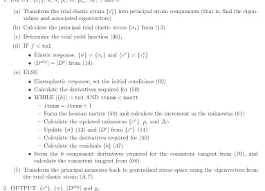
where the pre-superscript denotes the iteration number. The Newton–Raphson iterative process continues until the residuals converge to within a given tolerance. Throughout the stress return, all of the derivatives are evaluated at the current state. This requires the repeated evaluation of the derivatives at each iteration. The full sequence for the stress return is given inFig. 11whereiindicates the current iteration number. The pseudo code for this algorithm is supplied inFig. 12.

3.1. Stress return error analysis

The accuracy of the stress return algorithm was assessed over the range 16q_t/q_y610 and

p

/66h6

p

/6 forp_t=pcn¼0:1, 0.3,

0.5, 0.7 and 0.9 for three of the two-parameter models:

a

=

c

= 1 (MCC),

a

=

c

= 0.5 and

a

= 0.6,

c

= 0.9. qy is the deviatoric yield

stress under triaxial compression at a particular pressurep. A ref-erence pressure of 100 kPa, compressibility index of

j

= 0.01, initial elastic volumetric strain

e

e

[image:11.595.104.488.461.738.2]

v0¼0 and a shear modulus ofG= 2 MPa

Fig. 12.Pseudo code for the two-parameter family of Critical State models. The tolerance (tol) was typically set to 11012

were used for the material’s elastic properties. pcn¼200 kPa,

M= 0.6,

q

e_{¼0:8 andk= 0.1 define the yield surface. The starting}

point for the error analysis was a hydrostatic stress state equal to the pressure under consideration. The constitutive model then was subjected to a deviatoric elastic strain increment correspond-ing to the elastic trial stress state. The return stress from this scorrespond-ingle strain increment was compared with the solution obtained by splitting the strain increment into 1000 sub-increments.

The following error measure was used to assess the accuracy of the stress return algorithm

e¼

ffiffiffiffiffiffiffiffiffiffiffiffiffiffiffiffiffiffiffiffiffiffiffiffiffiffiffiffiffiffiffiffiffiffiffiffiffiffiffiffiffiffiffiffiffiffiffiffiffiffiffiffiffiffiffiffiffiffiffiffiffiffiffi

f

r

rg f

r

eg

f gTff

r

rg f

r

egg q

ffiffiffiffiffiffiffiffiffiffiffiffiffiffiffiffiffiffiffiffiffiffi

f

r

egTf

r

eg

q ; ð63Þ

where {

re

} is theexactstress return corresponding to the sub-incre-mented solution and {

rr

} is the single increment BE return stress.

Stress iso-error maps are given inFig. 13for (i)

a

=

c

= 1 (MCC), (ii)

a

=

c

= 0.5 and (iii)

a

= 0.6,

c

= 0.9. Errors up to 28.0% appear for the

a

=

c

= 0.5 model atpt=pcn¼0:9 whenqt/qyis close to 10; this is

not unexpected for such a large strain increment. For the same model atpt=pcn¼0:3, the maximum error is less than 3.3%. All of

the models have an error less than 5% forqt/qy< 2. For the majority

of the pressure ratios (the exception being MCC forp_t=p_cn¼0:1), higher errors (within a particular sextant), are seen near the com-pression meridians due to the higher curvature in the yield surface. The region of the lowest error, for all models, is near thecentreof the yield surface (p/pc’

c

/2) where there is lower meridional

[image:12.595.64.519.178.728.2]

cur-vature in the surface and the direction of plastic flow is near iso-choric. For pt=pcn¼

c

=2 there is no error associated with the BE

Fig. 13.Errors associated with the iterative BE stress return for five pressure ratios (A)p/pc= 0.1, (B)p/pc= 0.3, (C)p/pc= 0.5, (D)p/pc= 0.7 and (E)p/pc= 0.9 for (i)a=c= 1, (ii)

return, as shown byFig. 13(i) sextant (C). In this case the trial stress will return radially onto the original yield surface at the intersec-tion with the Critical State following isochoric plastic flow. The highest errors are in regions of high curvature and high volumetric plastic flow. The maximum error (emax), maximum number of

iter-ations required to find convergence (itmax) and the largest change

in the size of the yield surface (Dp_cmax) are given inTable 1for all three of the models under consideration. For the MCC model, the maximum error of 24.1% occurs atpt=pcn¼0:1. In the lower

pres-sure ratios, the yield surface of the MCC model softens more than the other models. The opposite is seen for the high pressure ratios, with greatest errors and the largest hardening of the yield surface associated with the

a

=

c

= 0.5 model.Fig. 13andTable 1confirm the well-behaved nature of the integration scheme for the two-parameter family of Critical State models.

4. Consistent tangent

The use of the consistent tangent within the global Newton– Raphson (N–R) iterations allows for asymptotic quadratic conver-gence for the residual out-of-balance force [40]. In this section we present the consistent tangent for the family of hyperplastic models with a W–W LAD deviatoric section. That tangent is de-fined as

½Dalg ¼

r

;ee

t h i

: ð64Þ

It is obtained through minimising the residuals(47)with respect to the trial elastic strain,f

e

e

tg. The first row of(47)becomes

½bCe_fd

_r

_{^g þ}

_Dc

_½g^;

rrfd

r

^g þ f^g;rpcgdp^c

þdDcf^g;_rg ¼ fd^

e

e

tg; ð65Þ

whereð^Þdenotes six component vectors and matrices. Considering the second row, we obtain

dpc ðp~c;pcÞdpc f

^ ~

pc;rgTfd

r

^g ðp~c;DcÞdDc¼0: ð66Þ Finally the third row, from the consistency condition, yields

f^f;rgTfd

r

^g þf;pcdpc¼0: ð67Þ

Combining(65)–(67), we have

½Cbe _þ

_Dc

_½^g;

rr

Dc

f^g;rpcg f^g;rg f^~pc;rgT 1 ðp~c;pcÞ ð~pc;DcÞ

[image:13.595.30.554.87.162.2] [image:13.595.307.547.384.722.2]

f^f;rgT f;pc 0 2 6 6 4 3 7 7 5 |fflfflfflfflfflfflfflfflfflfflfflfflfflfflfflfflfflfflfflfflfflfflfflfflfflfflfflfflfflfflfflfflfflfflfflfflfflfflfflffl{zfflfflfflfflfflfflfflfflfflfflfflfflfflfflfflfflfflfflfflfflfflfflfflfflfflfflfflfflfflfflfflfflfflfflfflfflfflfflfflffl} ½Aalg1

fd

_r

^_g

dpc dDc 8 > < > : 9 > = > ;¼

fd^

_e

e

tg 0 0 8 > < > : 9 > = > ;:

ð68Þ

Multiplying both sides of(68)by [Aalg_{], we obtain}

fd

r

^g dpc dDc 8 > > > < > > > : 9 > > > = > > > ; ¼

½Dbalg _fAalg

12g A

alg

13

fAalg21g

T

Aalg22 A

alg

23

fAalg31g

T

Aalg32 A

alg 33 2 6 6 6 6 4 3 7 7 7 7 5

fd^

e

e

tg 0 0 8 > > > < > > > : 9 > > > = > > > ;

; ð69Þ

where½Dbalg_{is the six-component algorithmic consistent tangent.}

The six-component vectors and matrices required in(68)are given by

f^g ¼ fg f0g

and½g^;rr ¼

½g;rr ½0 ½0 2A2½I

" #

: ð70Þ

The consistent tangent from(69) must be transformed (through

(A.7)) using the eigenvectors associated with the trial elastic strain to obtain a stiffness matrix consistent with the six component stres-ses and strains.

5. Numerical analysis

5.1. Material point analysis

In this section we make comparisons with experimental data using two examples from the two-parameter family of Critical Table 1

Error and return quantities associated with the iterative BE stress return for the five pressure ratios inFig. 13fora=c= 1,a=c= 0.5 anda= 0.6,c= 0.9.

pt=pcn a=c= 1 a=c= 0.5 a= 0.6,c= 0.9

dpcmax=pcn itmax emax dpcmax=pcn itmax emax dpcmax=pcn itmax emax

(A) 0.1 11.74% 7 24.08% 4.48% 7 9.35% 9.36% 7 20.889

(B) 0.3 4.35% 8 8.46% 1.28% 8 3.25% 3.29% 7 6.759

(C) 0.5 0.00% 8 0.00% 5.38% 8 13.65% 0.93% 8 1.909

(D) 0.7 3.09% 7 6.28% 8.18% 9 21.57% 4.05% 8 8.529

(E) 0.9 5.18% 7 11.62% 9.18% 8 28.02% 6.19% 8 14.239

State hyperplastic models. A reference pressure of 100 kPa, com-pressibility index of

j

= 0.0073, initial elastic volumetric strain

e

e

v0¼0 and a shear modulus ofG= 4 MPa were used for the

mate-rial’s elastic properties. pc= 233.3 kPa, M= 0.964, k= 0.0447 and

qe

¼0:729 define the yield surface, as obtained by Dafalias et al.

[image:14.595.49.287.272.478.2]

[17](note that Dafalias used a linear relationship between void ra-tio and the logarithm of effective pressure rather than the bi-logarithmic relationship adopted in this paper, resulting in different values for

j

andk).

Fig. 14illustrates the material responses given

a

=

c

= 1 (MCC) and

a

= 0.3,

c

= 0.9 under drained triaxial compression for six over-consolidation ratios (OCR = 1, 1.25, 1.5, 2, 4 and 10). The re-sults are compared against experimental data from Gens[20]. In these tests, the material was initially under a hydrostatic stress state withp= 233.3, 186.7, 155.6, 166.7, 58.3 and 23.3 kPa, corre-sponding to the six OCRs. The material was subsequently com-pressed axially whilst maintaining a constant lateral pressure. The two-parameter model with

a

= 0.3,

c

= 0.9 provides an

[image:14.595.88.515.528.732.2]

im-proved fit over the MCC model to the experimental data (for all OCRs) in terms of (

r3

r1

)/2. These results illustrate the benefits of the yield surface having a form where the envelope is contracted towards the Critical State line whenq/p>M(recallFig. 3).

Fig. 15shows the drained triaxial compression stress paths for four OCRs together with the cumulative plastic work and energy dissipation for the same two-parameter model. For overconsolida-tion ratios less than 2/

c

, hardening takes place and the plastic work is greater than the dissipated energy. Whereas for overconsolida-tion ratios greater than 2/

c

, softening occurs and the converse is true. The rate of plastic work and plastic dissipation are given by

(11) and (7), respectively, where

v

ij= (

c

pc/2)dij and

uij

=

rij

v

ij.

When the hydrostatic pressure,p, drops below

c

pc/2, the product

of the shift stress with the plastic strain rate becomes negative (due to the dilative plastic strains) resulting in the total plastic work being less than the dissipation.

5.2. Strain probing

The concepts of stored plastic work and dissipation are illus-trated further in Fig. 16which presents Gudehus plots [24] for

a

= 0.6 and

c

= 0.9. A reference pressure of 100 kPa, compressibility index of

j

= 0.0073, initial elastic volumetric strain

e

e

v0¼0 and a

shear modulus of G= 4 MPa were used for the material’s elastic properties.pc= 233.3 kPa,M= 0.964,k= 0.0447 and

qe

¼0:729

de-fine the yield surface.

The model is subjected to 832 strain probes for 64spheres start-ing at different locations on the yield surface. Each spherehas a strain radius of 1000

l

(that is, 1103

). The directions of the indi-vidual strain probes are obtained using the HEALPix software[22], dividing the surface of the sphere into equal area patches.

Figs. 16(i) and (ii) show the stress response (known as Gudehus plots [24]) to these strain spheres. The Gudehus surfaces are shaded according to the degree of (i) dissipated and (ii) stored plas-tic work. The maximum and minimum work for each stress surface are scaled to 1 and 0. These correspond to 164.6 J/m3_and

68.8 J/ m3_{, respectively.}

Fig. 17presents a sequence of Gudehus plots for the model with the same material parameters as above but with pc= 300 kPa. Fig. 17(i) shows results in the

rx

–

ry

plane. Fig. 17(ii) gives the same plots viewed in the deviatoric plane. The model starts at a randomly selected point on the yield surface and is subjected to Fig. 15.Drained triaxial compression stress paths showing the cumulative plastic

work and dissipation for the two-parameter model witha= 0.3 andc= 0.9.

Fig. 16.Three dimensional Gudehus stress plots with shading according to (i) dissipated plastic energy and (ii) stored plastic energy. The maximum and minimum work for each stress surface is identified by 1 and 0 corresponding to 164.6 J/m3

and68.8 J/m3

[image:15.595.88.509.66.276.2]

Fig. 17.Sequence of Gudehus stress plots demonstrating the robustness of the BE stress return algorithm for (i)rx–ryplane and (ii) deviatoric view. The surfaces are shaded according to the length of the stress path with the maximum and minimum length identified by 1 and 0, respectively. Five of the 200 Gudehus plots are presented for steps 1 (A), 50 (B), 100 (C), 150 (D) and 200 (E).

[image:15.595.110.476.346.730.2]

1,280 strain probes in directions determined by HEALPix. Once again, the probes are each of length

ffiffiffiffiffiffiffiffiffiffiffiffiffiffiffiffiffiffiffiffiffiffiffi fDegTfDeg q

¼103

. The stress responses and internal material parameters are stored before advancing to the next Gudehus plot. One of the probe responses is randomly chosen as the starting point for the next strain sphere. Five of the 200 stress responses are plotted for probes 1, 50, 100, 150 and 200, where the surfaces are shaded according to the dis-tance from the starting stress state to the return stress state. The stress path between the starting points for the strain spheres is also plotted. As the pressure increases so does the elongation of the stress response. This is due to the pressure-sensitive nonlinear elasticity providing an increase in stiffness with pressure. The stress responses, when inside the yield surface, have a circular deviatoric section due to the elastic isotropy. The Gudehus plots are flattened in the direction of the yield surface as most of the strain increment is taken up by the plastic response, leaving little for the elastic (and hence stress) response. The smoothness of the stress return surfaces shown inFig. 17serves to demonstrate the well behaved nature and robustness of the implemented con-stitutive model.

5.3. Influence of f

The form of the yield function,f, significantly affects the robust-ness and efficiency of the BE stress integration method. The func-tion given by (36)1 (with

q

e¼1) is quite different to that used

by Collins et al.[7–9,11]who adopted the form

f¼ðp

cp

c=2Þ

2

A2 þ

q2

B21¼0: ð71Þ

Manipulating(23)we can obtain any number of different forms of the yield function in dissipative stress space. Through one such manipulation, we can obtain the yield function in dissipative stress space as

fu_¼ðpuÞ

4

A4 1 qu

ð Þ2 B2

!2

¼0; ð72Þ

which transforms to become

f¼ðp

cp

c=2Þ

4

A4 1

q2

B2

2

¼0 ð73Þ

in true stress space.(26), (71) and (73)describe the same yield sur-face. However, the nature of the yield function outside of the yield surface (f> 0) is very different for the three cases.Fig. 18shows con-tours offoutside the yield surface for (i)(71), (iii)(36)1and (iv)(73)

when

a

=

c

= 0.5 and

qe

¼1. Note that these plots have been made for the case where no LAD is present. Thus the deviatoric stress re-turn is radial in this illustrative example. When 10 <f< 200, the contours are plotted in intervals of 10. For(71),Fig. 18(i), we see a local minimum around (p/pc) =3 and very high local curvature

plus a maximum around (p/pc) = 0.5 (see detail in Fig. 18(ii)).

The presence of these minima and maxima could cause significant problems for a BE stress return algorithm. These difficulties are completely removed by using(36)1; seeFig. 18(iii).(73)contains

[image:16.595.311.444.115.187.2] [image:16.595.60.522.393.739.2]

negative regions outside the yield surface, as shown inFig. 18(iv). If a trial stress state is located within one of these regions then the constitutive model falsely predicts a purely elastic response de-spite the stress being outside the yield surface.

Fig. 19shows stress returns for the three forms off:(36)1,(71) and (73). A reference pressure of 100 kPa, compressibility index of

j

= 0.01, initial elastic volumetric strain

e

e

v0¼0 and a shear

modu-lus of G= 2 MPa were used for the material’s elastic properties.

pc= 200 kPa,M= 0.6,k= 0.1,

a

= 0.5,

c

= 0.5 and

qe

¼1 define the

yield surface. The models are subjected to a trial elastic strain state, as given inTable 2, and their return paths observed. The size of the yield surface displayed inFig. 19corresponds to the finalpcnþ1value

from the stress return associated with(36)1.

In Fig. 19(i) the different returns associated with the three forms of the yield function are compared. The trial state has zero pressure. This provides a particularly challenging state from which to start a BE stress integration. The values of the trial yield function (ft), trial stress state ({

rt

}), final stress state ({

rn+1

}), final size of the

yield surface (pcnþ1) and the number of iterations to find

conver-gence are given inTable 2. The value of the yield function(73)at the trial state is negative, thus the constitutive model predicts an elastic response, which is clearly incorrect for that trial stress.

(71)fails to converge after 24 iterations and the size of the yield surface takes a meaningless negative value. The stress state after the 24th iteration is denoted by {24

_r

err_{}. The return path oscillates}

either side of the stress origin, unable to converge to back onto the yield surface. Only the model with the yield function described by

(36)1converges to the appropriate stress state, although 19

itera-tions are required to converge within the specified tolerance. In

this case the yield surface has contracted (softened) to 27% of its original size due to the significant plastic dilation associated with the stress return.

Fig. 19(ii) and (iii) demonstrate stress returns for the yield func-tions described by(36)1and(73). For both trial states,(73)

con-verges to a stress (f

r

err

nþ1g) associated withf= 0 outside the yield

surface, rather than onto the correct yield surface. These false stress returns produce an inappropriatepcnþ1 value and give rise

to the incorrect consistent tangent matrix. (36)1 correctly

con-verges back onto the yield surface for both trial stress states in eight and six iterations (Fig. 19(ii) and (iii)), respectively.

The stress returns shown inFig. 19demonstrate the importance of using an appropriate form offfor the BE integration scheme, and confirm that(36)1provides a more robust expression than(71)(or (73)).

5.4. Single element test

[image:17.595.30.553.349.487.2]

A simple small strain finite element analysis was first under-taken to assess the constitutive model’s performance within a gen-eral purpose 3D code. A single unit-cube (8-noded hexahedral element) constrained on its lower horizontal and two vertical faces was initially subjected to a uniform hydrostatic pressure of

Table 2

Stress return values for different yield functions (seeFig. 19).

f ft fetg rt(kPa) {rn+1} (kPa) pcn+1(kPa) Iterations

(i) (36)1 9.4921019pa4 {0.156 0.0016 0.189}T 54.09 19

(71) 1.688102

0:1444

0:1100

0:0756 8 < :

9 = ;

137:78 0 137:78 8 < :

9 = ;

{137.54 0 137.54}T

6.787106

24 +

(73) 2.814104

{137.78 0 137.78}T

200 0

(ii) (36)1 4.7151021pa4 0:0294

0:0050 0:0394 8 < :

9 = ;

310:39 448:17 585:95 8 < :

9 = ;

{97.75 130.06 162.38}T

231.87 8

(73) 3.9639 {220.09 370.40 520.72}T

204.33 5

(iii) (36)1 3.4651020pa4 0:0104

0:0330 0:0171 8 < :

9 = ;

216:71 271:83 326:94 8 < :

9 = ;

{126.74 154.62 182.49}T

213.38 6

(73) 1.905 {128.82 206.09 283.37}T

[image:17.595.40.546.382.731.2]

206.35 7

100 kPa. Subsequently, a compressive vertical point load of 20 kN (or 10 kN for the

a

= 1,

c

= 0.5 model) was applied to the element’s unconstrained top corner (see diagram lower centre ofFig. 20(i)), via 10 equal loadsteps. A reference pressure of 100 kPa, compress-ibility index of

j

= 0.01, initial elastic volumetric strain

e

e

v0¼0 and

a shear modulus ofG= 5 MPa were used for the material’s elastic properties.pc= 100 kPa,M= 1,k= 0.1 and

qe

¼0:7 define the yield

surface.

Fig. 20(i) gives the force–displacement response for the models with no LAD and with the W-W LAD. Four combinations of

a

and

c

were investigated with the two parameters taking values of 0.5 or

1(the yield surfaces with the W–W LAD can be seen inFig. 7). In all cases the models with a W-W LAD produced softer results due to those envelopes being enclosed within the deviatorically circular non-LAD surfaces (that is, plastic straining started earlier in the LAD models). Due to the material being normally consolidated, with all stress points starting on the compressive nose of the yield surface, changing the values of

a

and

c

led to a significant effect on the load–displacement response. As shown inFig. 2, decreasing

a

and

c

had the effect of increasing and decreasing the deviatoric yield stress (forp>

c

pc/2), respectively. This led to a stiffening up

(for decreasing

a

) or softening down (decreasing

c

) of the load– displacement response.

Fig. 20(ii) shows the N-R convergence rate for the simulation with

a

=

c

= 0.5 and the W–W LAD dependency. This figure

demon-strates the asymptotic quadratic convergence of the procedure. The following measure of (residual) out-of-balance force

jffrgj ¼

ffiffiffiffiffiffiffiffiffiffiffiffiffiffiffiffiffiffiffiffiffiffiffiffiffiffiffiffiffiffiffiffiffiffiffiffiffiffiffiffiffiffiffiffiffiffiffiffiffiffiffiffiffiffiffiffiffiffiffiffiffiffiffiffiffiffi

ffextg ffintg

f gTfffextg ffintgg q

ð74Þ

was used to determine convergence, where {fext} and {fint} are the

external and internal forces, respectively.j{fr}jfor loadsteps 6–10

are given inTable 3.

5.5. Numerical verification: plane strain flexible footing analysis

Borja and Tamagnini[3]presented the small strain and finite deformation analysis of a 4 m flexible footing using the MCC con-stitutive model (with identical elasticity and hardening laws as adopted in this paper). While that analysis provides a rather sim-plified finite element simulation, it offers a useful comparison with which to validate the finite element framework and constitutive model described in this paper. Due to symmetry, only half of the domain (of width 2W= 40 m, depthH= 5 m and footing half width

[image:18.595.46.563.368.451.2]

bof 2 m) was discretised using 91 nine-noded plane strain quadri-lateral elements with nine-point Gaussian quadrature (as shown in

Fig. 21). This is the same structured mesh as used by Borja and Tamagnini [3]. The MCC constitutive model used the following parameters: M= 0.857,

j

= 0.0177, k= 0.115,

qe

¼1:0 and

G= 5.4 MPa.

Table 3

Normalised residual out of balance forcej{fr}jvalues for the final 5 steps of the single 3D finite element simulation with the W–W LAD (a=c= 0.5).

Iteration Loadstep

6 7 8 9 10

1 1.5414e+03 1.6129e+03 1.6521e+03 1.6667e+03 1.6642e+03

2 8.6364e+02 9.5251e+02 1.0205e+03 1.0659e+03 1.0894e+03

3 4.3344e+01 5.3360e+0 5.7849e+01 5.8497e+01 5.7817e+01

4 3.4309e01 3.9938e01 3.6357e01 3.3166e01 3.0497e01

5 1.7303e05 1.7602e05 1.4240e05 1.1491e05 9.3213e06

[image:18.595.149.459.481.729.2]

6 3.7738ell 3.6956ell 3.3056ell 3.0253ell 4.6145ell

The two-parameter model (of which MCC is a special case) was implemented within a Lagrangian finite deformation finite element code. The use of a logarithmic strain-Kirchhoff stress formulation, combined with an exponential map of the plastic flow, allows the incorporation of existing small strain constitutive algorithms without modification. See[16]and the references contained within for more details on the finite deformation formulation. Borja and Tamagnini [3] derived the following relationship between the small strain (Cauchy) and finite deformation (Kirchhoff) compress-ibility indices

~

j

fd¼

j

1

j

and~kfd¼

k

1k; ð75Þ

whereð~fdÞidentify the finite deformation parameters. These

rela-tionships should be used to obtain the compressibility indices appropriate for finite deformation analysis based on a logarithmic strain-Kirchhoff stress formulation, as used in the recent paper by Yamakawa et al.[44].

The drained finite element simulation started from an initial overconsolidated state generated using the following small strain numerical procedure:

1. apply gravitational loads corresponding to a saturated weight of 10 kN/m3_{assuming a reference pressurep}

r= 1 kPa,

2. impose a uniform surface surcharge of 5 kPa, then 3. remove the surface surcharge.

The initial elastic strains {

e

e_{} and the size of the yield surfacep} c

for the flexible footing analysis were set equal to those obtained from the above procedure. The nodal displacements were reset to zero for the finite deformation analysis and the elastic volumetric strains increased by

j

~

e

e

vto account for the change in

j

between

Cauchy and Kirchhoff stresses. A vertical pressure of 90 kPa was applied over the half-width of 2 m in 90 equal loadsteps.

The pressure-centreline displacement response is shown in

Fig. 21. The finite element response shows excellent agreement with the results presented by Borja and Tamagnini[3](shown by discrete points). This analysis verifies the numerical procedure for both the implemented constitutive model and the finite defor-mation framework.

5.6. Plane strain rigid footing analysis

[image:19.595.41.272.192.453.2] [image:19.595.134.451.491.738.2]

A plane strain incremental small strain finite element analysis of a 1 m wide rigid strip footing bearing onto a weightless soil was performed to assess the model’s performance within a more complex finite element problem. Due to symmetry, only one half of the problem was considered. The same finite element discretisa-tion as presented in [18]was used. The mesh had a depth and Fig. 22.Rigid strip footing plane-strain finite element discretisation.

width of 5 m (seeFig. 22). 135 eight-noded quadrilaterals, with re-duced four-point quadrature, modelled the problem. The footing was assumed to be rigid and smooth with an imposed vertical dis-placement of 300 mm, supplied via 100 equal increments. A refer-ence pressure of 100 kPa, compressibility index of

j

= 0.0322, initial elastic volumetric strain

e

e

v0¼0 and a shear modulus of

G= 2.329 MPa were used for the material’s elastic properties.

pc= 400 kPa,M= 0.3640,k= 0.161 and

qe

¼0:7953 (/= 20°) define

the yield surface. Four yield surfaces were investigated:

a

=

c

= 1 and

a

= 0.6,

c

= 0.9 with and without a W–W LAD.Fig. 23presents the pressure–displacement response of the footing for the four constitutive models. Reducing

a

and

c

leads to a softer response, as does introduction of the LAD. The load required to obtain a dis-placement of 300 mm reduced by 87.8% for both the MCC and

a

= 0.6,

c

= 0.9 models.

The convergence of the footing problem for

a

= 0.6,

c

= 0.9 with the W–W LAD is presented inFig. 24for displacements 30, 60, 150, 240 and 300 mm. The out-of-balance force was determined using

(74), normalised with respect to the norm of the external force vec-tor, with a tolerance of 109_{. Despite the imposed relatively large}

displacement increments, the convergence analysis demonstrates the robustness and efficiency of the global Newton–Raphson solu-tion scheme when using the algorithmic consistent tangent. The

number of elasto-plastic Gauss points (npgp) is also given for each

displacement. The progressive development of plasticity is evident from these values.

5.7. Finite deformation cavity expansion

The final example is an analysis of the expansion of a cylindrical cavity under internal pressure. Although this is a one-dimensional axi-symmetric problem, we treat the expansion as a 2D plane strain finite element analysis. Only 3°of the domain (with a cavity internal radius of a0= 1 m and a fixed outer boundary of radius

b0= 2 km) is discretised using 150 four-noded plane strain fully

integrated quadrilateral elements. The size of the elements were progressively increased by a factor 1.1 from the inner to the outer surface. The internal radius (a) was expanded to 5 m via 200 equal displacement-controlled increments. In[16]this discretisation was shown to provide excellent agreement with the finite deformation analytical solution for Mohr–Coulomb.

A reference pressure of 100 kPa, compressibility index of

~

j

¼0:0322, initial elastic volumetric strain

e

e

v0¼0 and a shear

modulus of G= 2.329 MPa were used for the material’s elastic properties. pc= 600 kPa, M= 0.4235, ~k¼0:161 and

qe

¼0:7695

[image:20.595.72.531.324.488.2]

(/= 23°) define the yield surface for this simulation.

Fig. 24.Rigid strip footing convergence showing the norm of the residual out-of-balance force against the previous out-of-balance force for loadsteps 10, 20, 50, 80 and 100.

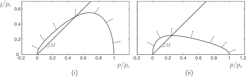
[image:20.595.77.537.529.741.2]

[image:21.595.83.506.68.329.2]

Fig. 25presents the internal pressure–displacement results for the same combination of constitutive models as analyzed in Sec-tion5.4.Fig. 25(i) and (ii) shown the results for the models with circular deviatoric sections and those with a W–W LAD, respec-tively. The W–W models have peak loads, on average, 86.1% lower than those seen in the models which are independent of the third invariant of stress.

Fig. 26(i) presents the convergence results for the final 5 load-steps of the simulation with

a

= 0.5,

c

= 1 and a W–W LAD. This fig-ure demonstrates the asymptotic quadratic convergence of the global finite deformation N–R procedure, where the measure of residual out-of-balance force is once again given by(74) norma-lised with respect to the norm of the external force vector. The con-vergence for the final loadstep is given inFig. 26(ii) where the norm of the residual out-of-balance force is plotted against the previous out-of-balance force. The gradient of this line indicates the conver-gence rate. The results demonstrate (for this case) super-quadratic convergence until the machine precision limit is attained.

6. Conclusion

In this paper we have presented for the first time the complete backward Euler stress integration expressions and consistent tan-gent for the Collins and Hilder family oftwo-parameter hyperplas-tic Crihyperplas-tical State constitutive models. The study includes incorporation of the elliptic Willam–Warnke Lode angle depen-dency on deviatoric yielding rather than the Matsuoka–Nakai LAD, as the latter can led to convergence difficulties under gener-alised stress increments (specifically, problems are introduced when any of the trial principal stresses are tensile).

After deriving all the expressions required for a material point algorithm, the performance of several variants of the family of models were examined. Drained triaxial compression simulations revealed improved realism over the modified Cam–Clay model for both normally and heavily over-consolidated states. Gudehus strain probe investigations provided a greater understanding of stored and dissipated plastic work for three dimensional stress

paths. The robustness of the BE stress return algorithm was dem-onstrated, for the first time, using a linked sequence of Gudehus plots where the constitutive model is subjected to a random path of strain probes. This provides a challenging but important test for any elasto-plasticity model, as any failure to return to the hard-ening/softening yield surface, when exploring the full strain space, can be identified immediately.

The influence of the yield function on the implicit stress inte-gration procedure was examined. Three forms offthat describe the same yield surface were explored. These formulations were subjected to identical trial elastic strains and their return paths ob-served. The tests confirm the well-behaved robust nature of the BE stress return algorithm using the new form of the yield function

(36)1.

Embedding the constitutive models within a Lagrangian finite element finite deformation numerical scheme allowed more demanding analyses to be performed. In each of the 22 simula-tions, the use of the consistent algorithmic tangent led to rapid convergence of the global Newton–Raphson nonlinear solution scheme. In all examples, the model and finite deformation code be-haved stably. Further work is now required to develop a robust two-surface anisotropic version of this attractive hyperplastic Crit-ical State framework in order to capture inelastic orientational changes to the material fabric and reproduce hysteretic effects (in a more convincing fashion) under cyclic loading.

Appendix A

A.1. Stress derivatives

This paper is concerned with isotropic constitutive equations, thus the following derivatives need only be formed with respect to the principal stresses. The derivatives ofJ2andJ3are given by

fJ2;rg ¼ fsg

q

andfJ3;rg ¼fs2s3 s1s3 s1s2gTþ

J2

3f1g

where

q

¼ ð2J2Þ 1=2

: ðA:1Þ