Local pre-processing for node classification in networks : application in protein-protein interaction

for Node Classification in Networks

Application in Protein-Protein Interaction

Christopher E. Foley1,2_{, Sana Al Azwari}1_{, Mark Dufton}2_,

Isla Ross1_{, and John N. Wilson}1

1 _{Department of Computer & Information Sciences}

2 _{Department of Pure & Applied Chemistry}

University of Strathclyde, Glasgow, UK

Abstract. Network modelling provides an increasingly popular conceptualisation in a wide range of domains, including the analysis of protein structure. Typical approaches to analysis model parameter values at nodes within the network. The spherical locality around a node provides a microenvironment that can be used to characterise an area of a network rather than a particular point within it. Microenvironments that centre on the nodes in a protein chain can be used to quantify parameters that are related to protein functionality. They also permit particular pat-terns of such parameters in node-centred microenvironments to be used to locate sites of particular interest. This paper evaluates an approach to index generation that seeks to rapidly construct microenvironment data. The results show that index generation performs best when the radius of microenvironments matches the granularity of the index. Results are presented to show that such microenvironments improve the utility of protein chain parameters in classifying the structural characteristics of nodes using both support vector machines and neural networks.

1

Introduction

Connected topologies have emerged as a productive way of modelling a wide variety of social, technical and biological systems. Among other domains, the paradigm has been used to characterise social networks [1], protein structures and interactions [3], genetic control [20], market economies [21] and human and machine communi-cation [2]. The power and flexibility of the network concept is highly adaptable as a basis for explaining the overall behaviour of a system but an emerging theme of such modelling is the potential for identifying specific regions in a network that are of particular interest. Such hotspots might represent localised communities in social networks [1] or periods of excessive workload in computer networks [28]. In the remainder of this discussion, we focus particularly on networks that represent protein structural topology and hotspots that characterise points of interaction between proteins. However the novel concept presented here (i.e. the use of localisation to enhance the hotspot detection process) has potential for application in other domains modelled by networks.

M. Bursa, S. Khuri, and M.E. Renda (Eds.): ITBAM 2013, LNCS 8060, pp. 32–46, 2013. c

The physicochemical properties of proteins provide useful information that results in the identification of new drug targets. Virtual screening offers a methodology for processing entire data collections such as the Protein Data Bank (PDB)[9] with the aim of identifying useful new drug leads. However, it is important to design the screening process in such a way that the maximum benefit is extracted from the data available. An understanding of the structure of proteins and their data representation can guide the design of effective screening methodologies.

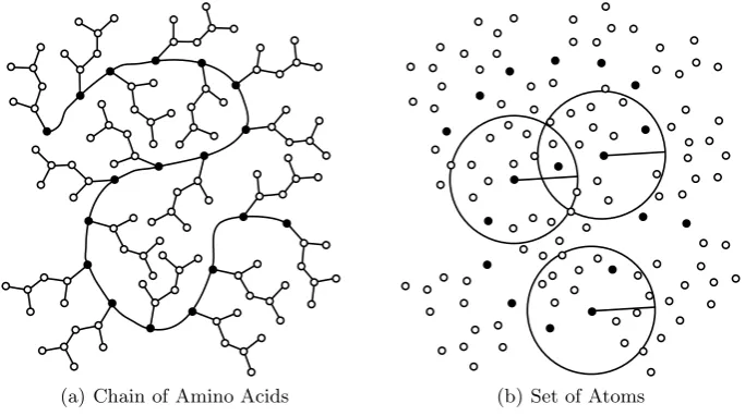
A protein is a chain (or combination of chains) of amino acid residues. The chain consists of a backbone that includes the α-carbon atom from each residue in the chain. Protein structures have been modelled as networks with the residues representing the nodes of the graph and edges representing residue interactions [3]. It is also possible to conceptualise nodes as discrete atoms in a protein structure with the edges representing inter-atom factors such as distance. The microenvironment that surrounds eachα-carbon is characterised by all the atoms in the network that fall within a defined sphere (Figure 1). Where mul-tiple chains are present, interactions may take place between the residues in different chains. Such protein-protein interaction sites contribute to the function of a protein. Consequently, prediction of the localities of interactions between proteins can be a guide to function prediction for a particular site [11]. Charac-terising the locality (rather than a point) in a protein structure can be addressed by evaluating microenvironments rather than the specific values associated with particular locations.

Proteins are made from the polymerisation of amino acids into a linear chain that is folded into a three dimensional (3D) structure. The folding pattern brings the functional parts of the protein together and adjusts its configuration in response to binding interactions. The positions of the atoms are determined by processes such as X-Ray Crystallography. Over 70000 3D protein structures are available from the PDB.

reveals the variation in 3D location of atoms in a protein as the temperature factor (B factor) parameter. Proteins are not rigid structures. In fact, much of the functionality of a protein depends on small positional adjustments. Tem-perature factor gives an indication of the likelhood of these adjustments taking place at each atom in the protein structure. The mean temperature factor of all the atoms enclosed in a microenvironment provides a value for this parameter that is based on the flexibility of the locality surrounding a singleα-carbon in a chain rather than the flexibility of a single point. This is a consequence of the dependence of the protein topology on the plasticity of the local struc-ture. Since any individual residue may be part of several spheres, pre-processing nodes in the structural network provides an estimate of the protein’s behaviour in the surrounding area rather than behaviour at the point represented by each node. This is useful because the activity of a protein is influenced by the gen-eral topology rather than point-by-point parameter values, that is in the gengen-eral context of networks, the structures behave as communities rather than a set of discrete nodes. The temperature factor of a particular residue represents only the flexibility at a specific node in the protein structure network. Other residue parameters such as hydrophobicity[11] (the extent to which the residue repels water) can be evaluated for microenvironments using a similar approach and together these parameters can be used to classify the residues in a chain on the basis of their likely contribution to protein-protein binding sites [10].

A range of processes are available for establishing classifications in datasets, however support vector machines (SVM) and neural networks (NN) typically span the range of prediction accuracies of such methods [10]. An SVM [14]

(a) Chain of Amino Acids (b) Set of Atoms

Fig. 1.Simplified representations of a protein.α-carbons are black and the side chain

atoms are hollow. Microenvironment spheres are defined around each of theα-carbons

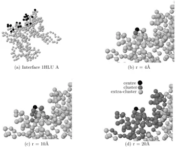
(a) Interface 1HLU A (b) r = 4˚A

(c) r = 10˚A

centre cluster extra-cluster

(d) r = 20˚A

Fig. 2. Amino acid residues clustered in the spheres of varying radii surrounding a single residue centre in the protein-protein interface

is a supervised learning mechanism that generates a hyperplane separating data in a training set. SVMs have been used in bioinformatic research to generate optimal classifications of sites on protein chains [13]. Artificial neural networks represent an alternative approach to classifying input data. They provide a means of deriving a functional model to separate classes in the input data. As with SVMs, NNs are able to classify non-linear data [33]. By training SVMs and NNs with sets of appropriate data, the likely positions of protein-protein interaction sites in a protein chain can be distinguished [24].

The contribution of the work described in this paper is to identify the best way of generating an on-the-fly index for the rapid association of nodes within a network. This methodology is then used to demonstrate that the assembly of clustered data makes a significant contribution to predicting hotspots in protein structure networks. In turn, this introduces the general approach of network analysis using localised topological summaries. The rest of the paper is organised as follows: Section 2 establishes the context of related approaches. Section 3 describes index generation and its use in the microenvironment assem-bly algorithm and presents the experimental work, the results of which are set out in Section 4. The paper concludes with an evaluation of the results and the potential for further work in Sections 5 and 6.

2

Related Work

Improvements in the performance of processing geometric data can be achieved by using specialised data structures. Scenes can be represented in hierarchi-cal trees of bounding volumes [22]. kd-trees are a common structure [8] and their traversal allows intersections to be calculated or distances to be measured. When working with point data, Voronoi diagrams [5] can be used to divide the n-dimensional space into sectors around each point. Using this approach, the entire space within each sector is closer to its parent point than to any other point. This is useful for queries that determine nearest neighbours. In apply-ing these principles to processapply-ing molecular data, early recognition of the power of quantising the space of individual molecules came from Leventhal [23]. This approach was further contextualised by Bentley [7] who assumed a quantisation based on search radius. The approach described in the current work explores the assumption that the optimum cell size of the quantisation is the same as search radius. Establishing the optimal approach is an essential step in providing a suitably efficient method of microenvironment assembly.

The novel idea presented here is that pre-processing network data by the con-struction of parameter aggregates within microenvironments improves the ability to identify hotspot nodes. This contrasts with previous research that focuses on point parameter data. The effectiveness of this approach is demonstrated using both SVM and NN classifiers in the prediction of protein-protein interface sites.

3

Prediction Model

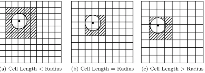
Microenvironment assembly determines the atoms that lie inside the sphere that is centred on each α-carbon in a protein chain. The simple approach of calculating the Euclidean distance between all residue/atom pairs is inefficient in a network that may consist of thousands of nodes. Cell partitioning [7] is used to pre-organise data so that only nearby atoms are considered as candi-dates during microenvironment assembly. Generation of the cell index is carried out on-the-fly having previously established the overall maxima and minima of spatial coordinates in the collection of protein structures and this is used to pro-duce a 3D grid. The coordinates of each atom associate it with a particular cell in this grid. The index identifies a candidate set of atoms that can be formed from the surrounding cells, immediately ruling out distant atoms from consideration. Only atoms within a reasonable distance of the sphere centre become candidates. The distances between the candidates and the sphere centre are calculated and the appropriate atoms included in the sphere. The index can be tuned by alter-ing the size of the 3D cells and Figure 3 shows how the candidate set is narrowed down by choosing only the cells that intersect with the sphere. Figure 4 gives a formal description of the index generation algorithm. Given the importance of this step in on-the-fly assembly of microenvironments, it is necessary to assess whether the optimal cell edge length is the same as radius size or whether a sub-multiple (L/n) of radius size would be more appropriate.

(a) Cell Length<Radius (b) Cell Length = Radius (c) Cell Length>Radius

1: Create a 3D array of cells encompassing all elements in the PDB.

2: foreach atom in the chaindo

3: Determine which cell this atom belongs in.

4: Place a reference to the atom in this cell.

5: foreach sphere centre in the chaindo 6: Create an empty sphere.

7: Determine which cell this sphere centres in.

8: calculate the length of the shaded area by

9: 2× sphere radius_{box length} + 1

10: foreach cell in the shaded areado 11: foreach atom in the celldo 12: distance =Δx2₊Δy2₊Δz2

13: if distance <sphere radiusthen 14: add this atom centre to the sphere

Fig. 4. 3D grid atom allocation algorithm

At one extreme, a single large cell will place all the atoms together, effectively removing any benefit from the index. At the other end of the spectrum, if the cell size is too small each atom will have its own box, negating the advantage. Figure 3 suggests that choosing a cell size that matches the sphere radius constrains the candidate space but that sub-multiples (L/2,L/3 etc.) might be more effective. A cell length equal to the microenvironment radius maximally constrains the candidate space volume for the smallest number of candidate cells. This volume can be constrained further by using a greater number of smaller cells. Adding another layer of cells reduces the optimum cell size to L/2. A further layer reduces it toL/3 and cell lengths for these volume minima can be generalised toL/n.

Experimental work was carried out to evaluate the optimal approach to indexing Protein Data Bank (PDB) data [9] with a view to rapid assembly of microenviroments. A second set of experiments evaluates the effect of physico-chemical parameter variation on the detection of hotspots within protein network structures.

3.1 Index Configuration

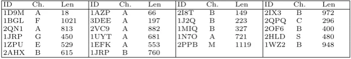
Table 1.Set of protein chains used for benchmarking the index algorithms

ID Ch. Len ID Ch. Len ID Ch. Len ID Ch. Len 1D9M A 18 1AZP A 66 2I8T B 149 2IX3 B 972 1BGL F 1021 3DEE A 197 1J2Q B 223 2QPQ C 296 2QN1 A 813 2VC9 A 882 1MIQ B 327 2OF6 B 400 1JRP G 450 1UYT A 681 1N7O A 721 2HLD S 480 1ZPU E 529 1EFK A 553 2PPB M 1119 1WZ2 B 948 2AHX B 615 1JRP B 760

The performance evaluation of microenvironment assembly was carried out by repeating the algorithm 1000 times. In order to make sure the compiled and optimised execution was measured, the 1000 measurements were repeated until two consecutive measurements were within 10% of each other. To prevent the benchmarked code being optimised out by the compiler, a summation of the sphere results was calculated and output to the console after the time measurements were complete. To determine the best cell size, the protein size was kept constant. Chain E from 1ZPU was chosen since it is in the middle of the range of chain length, which fixed the number of residues at 529.

An index using cells that are too small will take a long time to create while very large cells will approach O(n2_{) in terms of microenvironment assembly}

performance. Somewhere between these two extremes must lie the maximum efficiency. The experiment was run at sphere radii of 4, 5, 6, 7, 8, 9 and 10˚A. For each sphere size, the cell size was varied from 4 ˚A to 20 ˚A in steps of 1˚A. The best cell size was deduced from the above experiments and used to benchmark the cell index at sphere radii of 4, 5, 6, 7, 8, 9 and 10˚A for each chain length in the dataset.

3.2 Aggregating Parameter Values

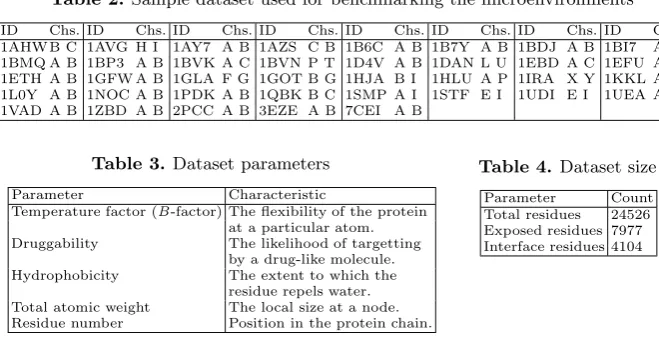
Table 2.Sample dataset used for benchmarking the microenvironments

ID Chs. ID Chs. ID Chs. ID Chs. ID Chs. ID Chs. ID Chs. ID Chs. 1AHW B C 1AVG H I 1AY7 A B 1AZS C B 1B6C A B 1B7Y A B 1BDJ A B 1BI7 A B 1BMQ A B 1BP3 A B 1BVK A C 1BVN P T 1D4V A B 1DAN L U 1EBD A C 1EFU A B 1ETH A B 1GFW A B 1GLA F G 1GOT B G 1HJA B I 1HLU A P 1IRA X Y 1KKL A H 1L0Y A B 1NOC A B 1PDK A B 1QBK B C 1SMP A I 1STF E I 1UDI E I 1UEA A B 1VAD A B 1ZBD A B 2PCC A B 3EZE A B 7CEI A B

Table 3.Dataset parameters

Parameter Characteristic

Temperature factor (B-factor) The flexibility of the protein at a particular atom. Druggability The likelihood of targetting

by a drug-like molecule. Hydrophobicity The extent to which the

residue repels water. Total atomic weight The local size at a node. Residue number Position in the protein chain.

Table 4.Dataset size

Parameter Count Total residues 24526 Exposed residues 7977 Interface residues 4104

To verify this assumption, a set of chain pairs with prior established protein-protein interaction sites was identified [4]. This set was further refined by removing chains containing multiple models (i.e. where variations in the configu-ration of the protein were possible) and those identified as containing significant redundancy [24]. Lastly, chains that had no matching pair subsequent to these steps were also removed. Following this process, the sample set consisted of those chain pairs shown in Table 2.

The residues in each chain of this set were then classified on the basis of their proximity to residues in the complementary chain. The occurrence of two α-carbons from complementary chains within a range of 12˚A was taken as an indication that the respective locations of these residues represented a protein-protein interaction site [24]. Theα-carbons in each chain were also classified on the basis of their accessible surface area (ASA) [19]. Surface residues were taken to be those with an ASA more than 20% of the surface area. The dataset chosen is summarised in Table 4.

A set of parameters indicated by previous work [16,26] was then derived for each surface residue in each chain. The parameters represent orthogonal charac-teristics of nodes within the network as shown in Table 3. Microenvironments of radii 0˚A to 50˚A were used to produce a mean value for each of these parameters for each node using the approach explained in subsection 3.1. For temperature factor and total atomic weight, each atom in the microenvironment provides a contribution to this mean. For other parameters used, each residue included in the locality provides a contribution.

set. A non-linear function provided the best separation for distinguishing protein-protein interaction sites using an SVM. Neural net classifiers were generated and tested using Matlab [25] and the same training and test sets as were used to generate the SVM classifications. As with the SVM classifiers, cross-validation was carried out within the training set during generation of the NN classifiers.

4

Experimental Results

The performance of microenvironment assembly based on a properly configured cell index is shown in Figure 6. The maximum number of amino residues in a single chain in the PDB is 4128, suggesting that index generation will be around 0.6 seconds in the worst case.

It can be seen from Figure 7, that the most efficient cell size is equal to the sphere radius. As the cell size increases from this global minimum, the time for the algorithm to run increases steadily. This is consistent with the larger cells holding progressively more atoms and therefore requiring more distance calculations. As the cell size decreases from the global minimum, the trend is for the time to increase. This is because more cells are required and their creation becomes the most time-intensive step. However Figure 7 also shows local minima at half the optimum cell size. Consider determining the sphere at a 7˚A radius. When the cell size is also 7˚A, the candidate list is drawn from the central cell and all of the surrounding cells. If the cell size is decreased to 6˚A we still have to check the central cell and the surrounding ones. However, now the range of the sphere can include atoms up to two cells away. If we go below 3.5˚A (half the optimum box size), we have to consider atoms three cells away. One could expect another local minimum at 1.75˚A, another at half this, and so on. The results from the optimum configuration are shown in Figure 8. Microenvironment assembly using the 3D grid index differs in that the speed varies with the sphere size.

The impact of changing the radius of the sphere on the identification of hotspot nodes in the context of their contribution to protein-protein interfaces is shown in Figures 9 and 10. The precision and recall of both SVM and NN show a gradual increase over the sphere radius from 0˚A to 40˚A. This variation can be seen more clearly in the context of the prediction accuracy shown in Figure 10. The SVM approach shows a peak accuracy of about 80% occuring at a radius of 40˚A. NN accuracy also peaks at the same radius. To explore the distribu-tion of data contributing to these predicdistribu-tions, Figure 11 shows the coefficient of variation (the ratio of standard deviation to mean) for each parameter over the radii chosen. Figure 12 shows the impact of isolating the contribution of each parameter to the SVM prediction. Here the microenvironment radius was fixed at 40˚A except for the indicated parameter, which was varied in the range 0˚A to 50˚A.

Fig. 5. Residues contributing to the protein-protein interface superimposed on the temperature factor distribution for 1HLU A

0 0.1 0.2 0.3

0 500 1000 1500 2000

Time / s

Chain Length / Amino Acids

Fig. 6. Summarisation using the 3D grid index

Fig. 7.Effect of cell size on execution time for different sphere radii

Fig. 8. Index generation at different sphere radii. Cell sizes are set equal to the sphere radius.

Fig. 9.Precision and recall at varying microenvironment radii

Fig. 10.Accuracy at varying microen-vironment radii

Fig. 11.Coefficients of variation Fig. 12. Principal component analysis

5

Discussion

The experimental work verifies the assumption in constructing spheres in net-work structures, that the most appropriate cell length matches sphere radius. This result provides confidence in the optimal performance of microenvironment assembly, which is necessary for locating good classifiers within the search space. The on-the-fly approach is efficient enough to remove the necessity for materialis-ing microenvironments. This improves the utility of the method since it removes the need for predicting the combinations of parameters that can distinguish hotspot nodes. If a user interface must respond to a mouse click or a keystroke within 0.1 s, the 3D grid index continues to meet the criteria up to about 1200 residues for the higher sphere sizes and over 2000 residues for sphere sizes of 7˚A and under. This makes it feasible to build a direct manipulation interface to large networks such as those represented by the PDB and provides support for interactive data mining. The experiments show that the performance of the index depends on sphere size, with larger radii making the index less efficient.

In the context of network representations of protein structures, the improve-ment in prediction has the potential for focusing the selection of appropriate sites for targeting drug design aimed at protein-protein interfaces. The longer term consequences are cost reductions duringin vitroassay. An additional benefit is the potential for scanning a large collection of protein structural data (e.g the Protein Data Bank) with a view to identifying the sites in all the chains where protein-protein interactions may be taking place. Bulk scanning such as this necessitates the development of the optimised indexing approach described in Section 3.

The coefficients of variation suggest that the parameters chosen are subject to considerable variation in microenvironments that range from 0˚A to 20˚A. Beyond this, hydrophobicity and druggability show less variation. The results reported in Figure 12 suggest that despite restricted variation of these parameters beyond 20˚A, they still make an important contribution to the prediction process at microenvironment radii of around 40˚A.

This work has focused on the use of 3D coordinates to model protein structures as an example of nodes located within a network. Other approaches to protein modeling include representation as graph structures with edges typically denoting the spatial proximity of atoms within the structure [27]. In this idiom, microenvironments are an appropriate way of characterising the physicochemical topology of proteins because they can be parameterised to span variable sub-graphs within the chain. The utility of this approach is demon-strated in the increased classification accuracy for microenvironment centres. Other applications of graph theory include analysis of social network activ-ity, ecological systems and economic structures [1]. Within such domains, there is considerable challenge in the identification of communities as collections of interconnected nodes [34]. Search methodologies can be deployed to address this problem but they are typically limited in the range of network sizes that can be analysed. Microenvironments are an appropriate tool that can be applied in this context and we are currently developing our approach in this direction.

6

Conclusion

The experimental work reported has evaluated the efficiency of a parameterised 3D grid index for generating microenvironment data for use in the classification of residues in terms of their contribution to protein-protein interface sites. The index was evaluated with protein atomic coordinates and has been shown to be most efficient when the cell size matches the granularity of the summary.

References

1. Aggarwal, C.: Social Network Data Analytics. Springer (2011)

2. Ahlswede, R., Cai, N.C.N., Li, S.Y.R., Yeung, R.W.: Network information flow (2000)

3. Amitai, G., Shemesh, A., Sitbon, E., Shklar, M., Netanely, D., Venger, I., Pietrokovski, S.: Network analysis of protein structures identifies functional residues. J. Mol. Biol. 344(4), 1135–1146 (2004)

4. Ansari, S., Helms, V.: Statistical analysis of predominantly transient protein-protein interfaces. Proteins 61, 344–355 (2005)

5. Aurenhammer, F.: Voronoi diagrams-a survey of a fundamental geometric data structure. ACM Comput. Surv. 23, 345–405 (1991)

6. Bagley, S., Altman, R.: Characterizing the microenvironment surrounding protein sites. Protein Science 4, 622–635 (1995)

7. Bentley, J., Stanat, D., Hollins Williams, E.: The complexity of finding fixed-radius near neighbors. Information Processing Letters 6(6), 209–212 (1977)

8. Bentley, J.L.: Multidimensional binary search trees used for associative searching. Commun. ACM 18, 509–517 (1975)

9. Berman, H.M., et al.: The Protein Data Bank. Acta Crystallogr. D 58(6, pt. 1), 899–907 (2002)

10. Bisbal, J., Engelbrecht, G., Villa-Uriol, M.-C., Frangi, A.F.: Prediction of cerebral aneurysm rupture using hemodynamic, morphologic and clinical features: A data mining approach. In: Hameurlain, A., Liddle, S.W., Schewe, K.-D., Zhou, X. (eds.) DEXA 2011, Part II. LNCS, vol. 6861, pp. 59–73. Springer, Heidelberg (2011) 11. Burgoyne, N.J., Jackson, R.M.: Predicting protein interaction sites: binding

hot-spots in protein-protein and protein-ligand interfaces. Bioinformatics 22(11), 1335–1342 (2006)

12. Foley, C.E., AlAzwari, S., Dufton, M., Wilson, J.N.: Using microenvironments to identify allosteric binding sites. In: Proc. IEEE International Conference on Bioin-formatics and Biomedicine, pp. 1–5 (2012)

13. Chang, C., Lin, C.: LIBSVM: A library for support vector machines. ACM TOIST 2, 27:1–27:27 (2011)

14. Cortes, C., Vapnik, V.: Support-vector networks. Machine Learning 20, 273–297 (1995)

15. Csermely, P.: Creative elements: network-based predictions of active centres in proteins and cellular and social networks. Trends in Biochemical Sciences 33(12), 569–576 (2008)

16. Ezkurdia, I., Bartoli, L., Fariselli, P., Casadio, R., Valencia, A., Tress, M.L.: Progress and challenges in predicting protein-protein interaction sites. Briefings in Bioinformatics 10(3), 233–246 (2009)

17. Fariselli, P., Pazos, F., Valencia, A., Casadio, R.: Prediction of protein-protein interaction sites in heterocomplexes with neural networks. European Journal of Biochemistry 269(5), 1356–1361 (2002)

20. Kauffman, S.A.: Metabolic stability and epigenesis in randomly constructed genetic nets. Journal of Theoretical Biology 22(3), 437–467 (1969)

21. Kirman, A.P.: The economy as an evolving network. J. Evolutionary Eco-nomics 7(4), 339–353 (1997)

22. Klosowski, J., Held, M., Mitchell, J., Sowizral, H., Zikan, K.: Efficient collision detection using bounding volume hierarchies of k-dops. IEEE T. Vis. Comput. Gr. 4(1), 21–36 (1998)

23. Levinthal, C.: Molecular model-building by computer. Scientific American 214, 42–52 (1966)

24. Liu, R., Jiang, W., Zhou, Y.: Identifying protein-protein interaction sites in tran-sient complexes with temperature factor, sequence profile & accessible surface area. Amino Acids 38(1), 263–270 (2010)

25. MATLAB. version 7.13.0 (R2011b). The MathWorks Inc., Natick, Massachusetts (2011)

26. Shinji, S., Hiroki, S., Kobori, M., Noriaki, H.: Use of amino acid composition to predict ligand-binding sites. J. Chem. Inf. Model. 47, 400–406 (2007)

27. Vishveshwara, S., Brinda, K., Kannan, N.: Protein structure: insights from graph theory. Journal of Theoretical and Computational Chemistry 1(1), 1–25 (2002) 28. Wood, T., Shenoy, P., Venkataramani, A., Yousif, M.: Sandpiper: Black-box and

gray-box resource management for virtual machines. Computer Networks 53(17), 2923–2938 (2009)

29. Wu, S., Liu, T., Altman, R.: Identification of recurring protein structure microenvi-ronments and discovery of novel functional sites around cys residues. BMC Struct. Biol. 10(4) (2010)

30. Xia, J., Zhao, X., Song, J., Huang, D.: Apis: accurate prediction of hot spots in protein interfaces by combining protrusion index with solvent accessibility. Bioin-formatics 11(174), 1–14 (2010)

31. Gui, J., Yang, L., Xia, J.F.: Prediction of protein-protein interactions from protein sequence using local descriptors. Protein Pept. Lett. 17(9), 1085–1090 (2010) 32. Yuan, Z., Bailey, T.L., Teasdale, R.D.: Prediction of protein B-factor profiles.

Pro-teins: Struct., Funct., Bioinf. 58(4), 905–912 (2005)

33. Zhang, G.: Neural networks for classification: A survey. IEEE Transactions on Systems, Man and Cybernetics - Part C 30(4), 451–462 (2000)

34. Zhao, Y., Levina, E., Zhu, J.: Community extraction for social networks. Proc. National Academy of Sciences 108(18), 7321–7326 (2011)