City, University of London Institutional Repository
Citation:
Atkin, C.J. & Schrauf, G. (2000). Progress in linear stability methods for design applications. Paper presented at the European Congress on Computational Methods in Applied Sciences and Engineering (ECCOMAS 2000), 11-14 Sep 2000, Barcelona, Spain.This is the accepted version of the paper.
This version of the publication may differ from the final published
version.
Permanent repository link:
http://openaccess.city.ac.uk/14204/Link to published version:
Copyright and reuse: City Research Online aims to make research
outputs of City, University of London available to a wider audience.
Copyright and Moral Rights remain with the author(s) and/or copyright
holders. URLs from City Research Online may be freely distributed and
linked to.
PROGRESS IN LINEAR STABILITY METHODS FOR DESIGN
APPLICATIONS
Christopher J. Atkin* and Géza H. Schrauf †
*
Defence Evaluation and Research Agency (DERA) Farnborough, Hampshire GU14 0LX, UK
e-mail: [email protected]
† DaimlerChrysler Aerospace Airbus
28183 Bremen, Germany e-mail: [email protected]
Key words: laminar-turbulent transition, linear stability theory.
Abstract. Despite recent developments in the understanding of boundary layer receptivity
and non-linear stability, linear stability methods remain the state-of-the-art in industry for aerodynamic design and analysis. A conceptual model is presented to explain why the eN
1 INTRODUCTION
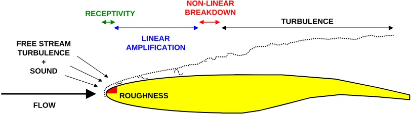
Since the recent revival of interest in laminar flow control for transport aircraft, the aerodynamic phenomenon of laminar-turbulent transition has received increased attention from the research community, resulting in significant developments in the understanding of, and ability to model, the transition process. There is much work to be done, but we now have an outline understanding of receptivity, the process by which perturbations are introduced into laminar boundary layer flows, and breakdown, the process by which non-linear interactions between large-amplitude perturbations eventually lead to turbulence. These two types of phenomenon occur at each end of the transition process and, provided that the disturbance environment outside the boundary layer is of a low level, the receptive and non-linear phases are separated by a lengthy region where the disturbances are governed by linear mathematics by virtue of their small amplitude. This summary is represented schematically in Figure 1.
RECEPTIVITY
LINEAR AMPLIFICATION
NON-LINEAR BREAKDOWN
TURBULENCE
FREE STREAM TURBULENCE
+ SOUND
FLOW
[image:3.612.100.506.296.410.2]ROUGHNESS
Figure 1: Schematic of boundary layer transition on a wing section.
In terms of fundamental research there is little to be added to our knowledge of the linear stability of boundary layers, except perhaps for the challenging problem of disturbances in three-dimensional boundary layers. The latest transition research presented at this Congress will concern new work in the fields of non-linear and secondary instability, adjoint methods, receptivity analysis and bypass transition. Why then are we reviewing linear stability theory in this paper? The answer is that, despite recent progress in transition research, linear stability methods remain the state-of-the-art in industry for airframe design and analysis. This is partly because of the lengthy validation period required before new computational methods are adopted for commercial use, but also because of the coherence between linear methods and the requirements of airframe design: at present, the kind of information needed to model accurately the receptivity and breakdown processes — such as environmental and surface finish data — is simply beyond the scope of the designer.
method can be used. For three-dimensional flows an arbitrary constraint, or integration
strategy, is required before the eN criterion can be applied — the choice of this strategy is still the subject of debate. In computational terms, linear stability analysis is expensive, and attempts have been made to develop simple short cuts which reduce this cost to acceptable levels. Finally, linear stability analysis is also very expensive in human terms since the modes of instability need to be specified before growth rates can be calculated: but there is no a
priori knowledge of which modes are the most likely to cause transition.
This paper reviews the latest results and conclusions from a series of recent collaborative projects, supported by the European Commission, which have contributed significantly to the confidence and ease with which linear stability methods can now be used for design.
2 LINEAR STABILITY APPLIED TO HIGH ASPECT-RATIO WINGS
2.1 Transition mechanisms for transport aircraft wings
The successful maintenance of laminar flow on a transport aircraft wing requires the control of three types of transition mechanism, as discussed by Schrauf1:
a) contamination of the wing attachment line flow by turbulence in the fuselage boundary layer (or, more rarely, natural transition of a laminar attachment line boundary layer); b) instability of the crossflow velocity profile, usually occurring just downstream of the
attachment line; and
c) instability of the streamwise velocity profile, usually occurring in the ‘roof top’ area of the wing pressure distribution.
The first mechanism is effectively a ‘show-stopper’ since it causes the complete wing boundary layer to be turbulent (barring the occurrence of re-laminarisation). Attachment line contamination is usually predicted using relatively simple empirical criteria since the number of influencing parameters is usually small2. The latter two mechanisms, crossflow (CF) and
Tollmien-Schlichting (TS) instabilities, occur over a large area of wing with varying local flow conditions and therefore require more sophisticated methods for the prediction of transition or the design of a laminar flow control system. Linear stability theory is therefore applied to the prediction of these two transition mechanisms.
2.2 Mathematics of local, linear stability analysis
The theory behind local, linear stability analysis has been well documented (see, for example, Arnal3). The scope of the analysis is usually restricted to three-dimensional flows on
infinite-swept wings, where the mean flow is assumed to be invariant in the spanwise direction. In practice the analysis is also applied without modification to real wings with moderate taper ratios.
(
) ( )
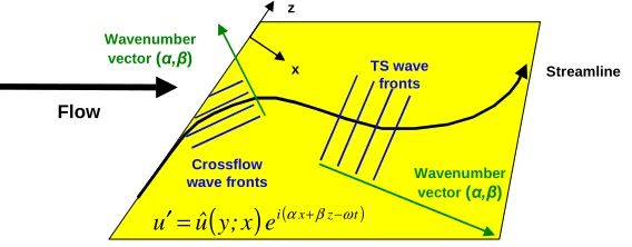
i( x z t) e y uˆ t , z , y , xu′ = α +β −ω (1)
where the prime indicates a perturbation quantity, u can represent any of the flow variables, t is the time co-ordinate and x and z are orthogonal spatial co-ordinates, usually aligned normal and parallel to the leading edge.
The stability equations contain terms of varying powers of Rδ, the local Reynolds number (effectively related to a local length scale, such as the boundary layer displacement thickness). The local stability equations are then obtained by neglecting all terms smaller than those of order O(1): this includes all curvature terms and the variation of the mean flow with the x co-ordinate. The wave amplitude function û therefore varies only with y. The approach is described as the parallel flow approximation since the divergence of the streamlines is not modelled. Solutions to the resulting stability equations (for simple swept-wing flows) can be obtained for combinations of real ω and β and complex α and û: the imaginary part of α constitutes an amplification rate in space and the complex nature of û simply accommodates variations in phase as well as disturbance magnitude.
Figure 2 illustrates the wave model as applied to crossflow modes and Tollmien-Schlichting modes on a transport aircraft wing. Crossflow modes are characterised by a wave-number vector (α, β) almost at right-angles to the local streamline and low frequencies
(including stationary modes) while Tollmien-Schlichting modes are characterised by higher frequencies and wave-number vectors aligned with the streamline (at least at modest Mach numbers). Crossflow modes tend to be amplified close to the leading edge, in regions of favourable pressure gradient, while Tollmien-Schlichting modes are most amplified in regions of adverse pressure gradient.
Flow
Wavenumber
vector (α,β)
Wavenumber
vector (α,β)
TS wave fronts Crossflow wave fronts Streamline x z
( )
i( x z t)e x ; y uˆ
[image:5.612.165.449.441.552.2]u′= α +β −ω
Figure 2: Schematic showing crossflow (CF) and Tollmien-Schlichting (TS) instabilities.
theory although this is not strictly rational in mathematical terms (since there are other terms of the same order still neglected). The addition of curvature to local methods did not, in fact, result in any improvements to the performance of the local theory4,5.
2.3 Mathematics of non-local, linear stability analysis
Despite the well-known work of Gaster6, Saric and Nayfeh7 and Herbert8 on non-parallel or non-local boundary layer stability, the use of these methods in Europe has lagged behind that
in the USA and their practical application in support of European laminar flow research has only recently been demonstrated9,10. In particular the EUROTRANS project10 was responsible
for the first systematic validation exercise for non-local methods and for the first non-local N-factor correlations. The non-local analysis starts with a more general substitution than the one shown in equation (1) above by allowing the amplitude function to vary slowly with x:
(
) ( )
i( x z t)e y , x uˆ t , z , y , x
u′ = α +β −ω (2)
The difference between local and non-local theory arises from the level of approximation made to the linear stability equations. The non-local stability equations retain terms which are of order O(Rδ-1): this includes the variation of both û and the mean flow with the x co-ordinate as well as terms involving the curvature of the co-ordinate system. The dependence of complex û on x leads to a new spatial amplification rate σ:
∂ ∂ + − = x uˆ uˆ 1 Real i u α σ (3)
where the precise value of σ depends on which flow parameter appears in formula (3) above. This difference between σ and αi, caused by the growth of the boundary layer, the curvature of the wing surface and the flow quantity used for measuring amplification, is the key difference between local and non-local linear stability theory from the point of view of transition prediction using the eN technique.
2.4 Integration of amplification rates: the N-factor; integration strategies
As described in section 2.2 above, local, linear stability analysis consists of a collection of eigenvalue problems, one for each combination of ω, β and spatial location. The solutions yield the local growth rates for each mode, but the modes at each station have to be logically connected in some way before the growth rates can be integrated to yield an N-factor:
( )
x[
x, , f( )
k]
dx N x 0 i k , i ′ = ′ =∫
= αω α ω β (4)
The angular frequency ω is taken to be constant for a given mode, but there are a number of relationships involving β, or integration strategies, which have been studied during the European laminar flow programmes:
B) constant wave number, αr2+β2 ;
C) constant spanwise wave number β; or
D) maximising the growth rate with respect to βat each station, i =0 ∂ ∂
β α
The first three options result in a two-dimensional array of N-factor curves, while the fourth option, termed the envelope strategy, simplifies the array so that, like the two-dimensional problem, the N-factor is a function only of frequency and spatial location.
The work load associated with calculating N-factor curves for all possible combinations of frequency and integration parameter k, options (A) through (C) above, is significant. Schrauf
4,5 has proposed a short-cut whereby option (A) is used for Tollmien-Schlichting modes, but
only for those modes where ψ= 0°, and option (B) is used for crossflow modes, but only for stationary modes (ω = 0). This strategy exploits two observations made during repeated analyses of experimental data during the European laminar flow programmes: firstly, that the amplification of Tollmien-Schlichting modes is quite insensitive to propagation direction near
ψ = 0°, and secondly that, for flight conditions at least, stationary crossflow modes tend to dominate because their initial amplitudes tend to be higher than those of the travelling (ω> 0) crossflow modes. These restricted N-factors are labelled NTS and NCF respectively.
Mack11 has demonstrated that option (C) is consistent with the spanwise similarity arguments used for high aspect-ratio wings, but all four of the integration strategies described above, plus the two-N-factor method, have been pursued: the ultimate selection criterion is the performance, in terms of consistency, of each integration strategy against experimental data.
Curiously enough, option (C) seems to have been adopted without challenge for the non-local theory10. The marching scheme used in PSE methods means that the ‘integration strategy’ issue, although it is not described as such in the PSE literature, has to be resolved before the stability calculations can even begin. With the local methods there is the opportunity to re-integrate already-calculated amplification rates according to different strategies, provided that the complete (ω, β) space has been investigated.
2.5 Explanation of the eN approach to transition prediction
We move from the mathematical details of the linear stability approach to a conceptual model which will explain why the eN approach is used and the circumstances under which it might be expected to work.
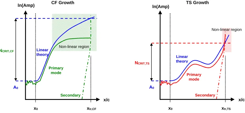
10% of the edge flow when non-linear effects set in. Figure 4 shows a similar image of Tollmien-Schlichting instability, although a region of stable flow is shown.
CF Growth
x/c
NCRIT,CF
x0 xtr,CF
Linear theory Secondary Primary mode ln(Amp) A0 Non-linear region
Figure 3: Schematic of CF instability growth.
TS Growth
x/c
NCRIT,TS
x0 xtr,TS
[image:8.612.102.512.157.347.2]Linear theory Secondary Primary mode ln(Amp) A0 Non-linear region
Figure 4: Schematic of TS instability growth.
What happens next has been deduced from experiments and numerical studies using advanced non-linear stability methods of the kind described by Casalis et. al.12. For crossflow modes, non-linear effects cause the instabilities to saturate at a given amplitude until secondary instabilities, as yet not well understood, develop. These secondary instabilities act extremely rapidly to cause breakdown to turbulence. The amplitude of Tollmien-Schlichting modes continue to increase roughly as predicted by linear theory, but at large amplitudes non-linear interactions (which are well-predicted by PSE-type methods10) generate higher harmonics which again grow much more rapidly than the primary modes. In both Figures 3 and 4, a blue line indicates the growth predicted by linear theory. This line follows the actual growth of the primary mode quite well for TS instabilities, but less well for CF instabilities.
The critical N-factor is measured as follows: a representative experiment is conducted for which the position of the neutral stability point x0 and the position of transition xtr can be measured or inferred, and for which the local linear growth rates (i.e. the slope of the blue line) can be calculated. The blue N-factor curve is then determined by integrating the growth rates between these two x-stations which thus define the ratio between the final and initial amplitudes: this critical N-factor is refined by considering all possible N-factor curves and selecting the most-amplified at transition. In a design situation, the neutral stability point x0 and the blue N-factor curve are known for each mode, allowing the position of transition xtr to be deduced from the critical N-factor.
but if these errors are typical of all applications, or at least well-defined categories of application, then the N-factor concept is useful. We would expect correlated N-factors to depend on the following real phenomena:
a) the disturbance amplitudes just upstream of the neutral point; b) the non-linear processes leading to breakdown.
The receptivity issue, (a) above, suggests that we would get different N-factors for tunnel tests as opposed to flight tests, and for an NLF (natural laminar flow, i.e. no suction) experiment as opposed to an HLF (hybrid laminar flow, i.e. with suction) experiment. The breakdown issue, (b) above, leads us to distinguish between experimental cases where transition is either dominated by crossflow modes, or by Tollmien-Schlichting modes, or by a mixture of the two. The following section describes how a series of experimental investigations have been used to investigate these different situations.
3 N-FACTOR CORRELATION AGAINST EXPERIMENTAL DATA
Each of the European laminar flow projects has involved either the design and execution of a significant experiment, or the analysis of the results for the purposes of N-factor correlation.
3.1 ELFIN project (1990-92)
In the ELFIN project, two experiments were conducted: a natural laminar flow (NLF) flight test using a glove on a Fokker 100 aircraft, and a hybrid laminar flow (HLF) test in the ONERA S1 wind tunnel. Both of these experiments were analysed using local theory during the ELFIN II project. The F100 tests have been thoroughly reported in the literature4,5 with the
following conclusions:
a) The envelope strategy, (D) above, was found to give a useful N-factor correlation when including compressibility and curvature effects.
b) None of the other single N-factor strategies, (A) through (C) above, were found to be particularly better than any of the others. They all suffered from ‘pathological’ test cases (30 out of the 60 analysed) where transition occurred downstream of the N-factor peak and, in some cases, in a region where all N-factors were decreasing.
c) For the two-N-factor strategy, options (B) and (C) were found to be effectively equivalent for determining crossflow N-factors NCF. The two-N-factor strategy also suffered from ‘pathological’ test cases.
Clearly, conclusion (a) is now challenged by the latest thinking on whether or not curvature terms are rational at the level of local stability theory.
3.2 ELFIN II project (1993-96)
crossflow instabilities. Aft of the front spar the fuel tank prevents the installation of suction ducting, etc., so the wing section is designed to generate a favourable pressure gradient that reduces the amplification of Tollmien-Schlichting waves and thus delays transition.
Figure 5: ELFIN II HLF wing instrumentation layout. Pressures were measured at DV stations and
[image:10.612.326.519.264.365.2]transition locations at CP stations using infra-red imaging over the shaded area.
Figure 6: ELFIN II HLF wing suction chamber and sub-chamber layout.
We first present one of the limitations of the envelope integration strategy (D) which becomes apparent for HLF applications. Figure 7 shows how the N-factor at transition changes directly with the applied suction rate. This occurs because the envelope strategy combines crossflow and Tollmien-Schlichting amplification rates: the effect of crossflow stabilisation by suction is thus felt by the transition N-factors even though the crossflow modes may play no part in the transition process. Special treatments for this effect have been suggested13 which involve including the averaged propagation direction in the N-factor correlation, but this may be a complication too far for adoption by industry users.
The approximate equivalence between strategies (B) and (C) for calculating crossflow
N-factors, observed in the F100 flight tests4,5, also applies to HLF experiments, as shown in
Figure 7: Effect of suction on envelope-strategy (D)
N-factors. Average suction velocities 0.2 m/s and
[image:11.612.325.511.129.302.2]0.15 m/s. ELFIN II HLF tunnel tests.
Figure 8: Comparison between (NCF, NTS) and
(Nβ, NTS) pairs. ELFIN II HLF tunnel tests.
3.3 Compressibility effects; sensitivity to Mach number
The geometry and the suction requirements of the ELFIN II wing were designed with incompressible stability theory because, at that time, most of the previous NLF and HLF experiments had only been evaluated with incompressible stability theory. Compressible theory was used only occasionally in more fundamental investigations. Even today many experiments have not yet been re-evaluated with compressible stability theory, for example the ELFIN I HLF tests in the ONERA S1 tunnel (1992). In order to provide data for the future application of compressible methods, the ELFIN II experiment was evaluated with both incompressible and compressible theory. As observed by many researchers, the effect of including compressibility terms is to reduce the amplification rates of TS waves, whereas the amplification rates of crossflow modes are less affected. The important point for design application is whether compressibility improves the correlation with experiment.
In Figures 9 and 10 we present a comparison of incompressible and compressible N-factor correlations. Figure 9 shows the mean value of the correlated NTS-factors computed for each of the five Mach numbers used in the tests. All cases have been considered except pure crossflow cases with an value of an incompressible NTS below three. The mean values were computed from a single case with M = 0.5, eleven cases with M = 0.6, five cases with M = 0.7, two cases with M = 0.78, and eleven cases with M = 0.82. We observe that the difference in N increases slowly with the Mach number. This trend holds for all except the highest Mach number, for which the difference becomes somewhat larger. Figure 10 contains the correlated
compressibility reduces NTS-factors by significant amounts but leaves the NCF-factors relatively unchanged. A closer inspection shows that this is also the case for this experiment. The trend towards the bottom left of the Figure is caused by cases with higher Mach numbers, as indicated by the black arrows. The shortest arrow on the left belongs to the case with the lowest Mach number of 0.5, the two other arrows to cases with M = 0.82. Furthermore, the inner edge of the band is not much moved towards smaller N-factors for pure crossflow cases. The NCF-factor for the crossflow case with lowest NTS-factor is reduced from 5 to 4.3: a shift of this size was expected from previous experiments.
Figure 9: Difference between compressible and
incompressible NTS-factors with increasing Mach
number. ELFIN II HLF tunnel tests.
Figure 10: (NCF, NTS) pairs from compressible and incompressible analysis. ELFIN II HLF tunnel tests.
3.4 Sensitivity to Reynolds number
In Figure 11 we plot compressible and incompressible NTS-factors against Reynolds number. Again we see that the cases with the smaller compressible N-factors are the ones with
M = 0.82. In this figure, we also include the linear regression lines for the incompressible and compressible values. The ‘incompressible’ regression line is closer to the horizontal than the ‘compressible’ one, i.e. the incompressible N-factors are more universal than the compressible ones. The same behaviour was observed for the ATTAS flight experiment14. In Figure 12 we plot the correlated crossflow N-factors for all cases with NCF > 3 against Reynolds number. The sensitivity to Reynolds number is much smaller for these N-factors. Interestingly, the latest A320 fin experiments show a completely different Reynolds number trend for
[image:12.612.101.293.243.406.2]Figure 11: Comparison of compressible and
incompressible NTS-factors with increasing
[image:13.612.324.516.431.590.2]Reynolds number. ELFIN II HLF tunnel tests.
Figure 12: Comparison of compressible and
incompressible NCF-factors with increasing
Reynolds number. ELFIN II HLF tunnel tests.
3.5 Comparison between ELFIN I and II tests
Comparisons of these wind tunnel results with the previously obtained results from the ELFIN Fokker 100 flight tests are shown in Figures 13 and 14. We see that, with incompressible as well as compressible instability theory, the correlated wind tunnel N-factor
Figure 13: Comparison between incompressible
N-factor pairs obtained from the ELFIN II HLF
tunnel tests and the ELFIN I F100 NLF flight tests.
Figure 14: Comparison between compressible
N-factor pairs obtained from the ELFIN II HLF
tunnel tests and the ELFIN I F100 NLF flight tests.
[image:13.612.98.284.433.593.2]encountered in the wind tunnel. These, in turn, generate instability waves with larger initial amplitudes which will induce earlier transition. Noise lowers the correlated NTS-factors, and the vorticity generated by the wind tunnel grids reduces the correlated NCF-factors.
Comparing the incompressible with the compressible results, we notice that compressibility reduces the difference between the correlated N-factors much more for the
[image:14.612.321.516.277.442.2]NTS-factors than for the NCF-factors. However we should keep in mind that comparing an NLF flight test with an HLF wind tunnel experiment is not straightforward: in the HLF experiment, the suction panel acts like a rough surface, causing larger initial amplitudes for the stationary crossflow vortices. At this point, we cannot know whether the difference in the NCF-factors is caused by the difference in the environment or by the greater surface roughness in the HLF experiment.
Figure 15: Comparison between incompressible
N-factor pairs obtained from the ELFIN II HLF
[image:14.612.97.286.281.440.2]tunnel tests and the ELFIN I HLF tunnel tests.
Figure 16: Effect of non-local terms on crossflow
N-factors. ELFIN I Fokker 100 NLF tests.
In Figure 15 we present the correlated N-factor pairs of the earlier ELFIN I HLF tunnel experiment obtained with incompressible stability theory. They compare well with the new results. The N-factor pairs from both HLF-experiments match well even though the former ELFIN I HLF experiment used a different type of pressure distribution. In addition to the differences in the pressure distributions, different boundary layer and stability codes were used for the stability analysis experiments. Because only an incompressible analysis was performed, no comparisons using compressible theory can be made.
3.6 Non-local theory N-factors
Not mentioned so far is the analysis of both the Fokker 100 NLF tests and the ELFIN II HLF tests using non-local, linear theory during the EUROTRANS project10. The first task in
Non-local theory was originally applied to improve the prediction of the critical Reynolds number (the neutral stability point) for the Blasius boundary layer. Practical application to
N-factor calculations, however, suggested that Tollmien-Schlichting N-factors were only slightly changed by the retention of the non-local terms. This is not true of crossflow
N-factors, particularly when investigating curvature effects which can only be correctly treated with non-local theory. Figure 16 illustrates the point using a typical stationary crossflow mode taken from one of the F100 test cases: here we see that the effect of the non-local terms (excluding curvature) are of the same order as the curvature effects, and act in the opposite
manner in terms of amplifying or damping the mode. Following these investigations it is now clear that the only correct treatment of curvature must involve a complete non-local analysis. Figure 16 also illustrates the different N-factors obtained from considering the u-velocity (normal to leading edge) or v-velocity (parallel to leading edge) perturbations.
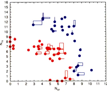
[image:15.612.101.513.382.563.2]Overall, the non-local theory results in lower crossflow N-factors than the local theory, as shown in Figure 17. In this case the peak crossflow N-factor (upstream of 15% chord) is reduced from 7.5 to 4.5 while the peak Tollmien-Schlichting N-factor (downstream of 15% chord) is increased slightly from 6.0 to 6.5. Note that a special local calculation has been carried out, using integration strategy (C) and involving all unstable modes (of which only a few are plotted). This work was conducted within the EUROTRANS project for the purposes of comparison with non-local theory, as discussed in section 2.3.
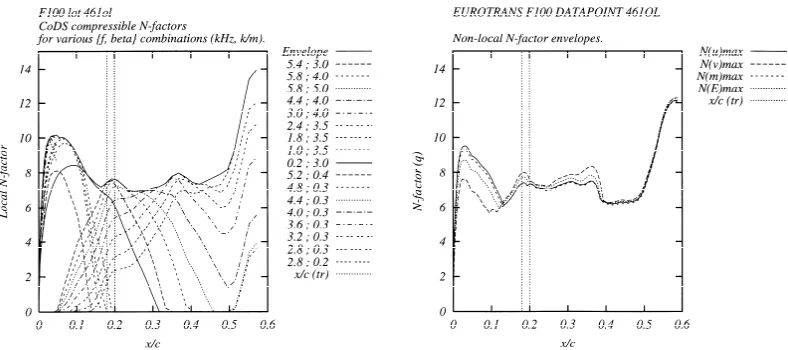
Figure 18: Local (integration strategy C, all modes) and non-local N-factors (maxima only) showing only minor changes in either crossflow or TS amplification. ELFIN I F100 case 461ol.
The effect of the non-local terms on crossflow N-factors is not consistent across all the test cases, as shown by Figure 18, which shows very little change to the N-factors in either the crossflow-dominated regions or the TS-dominated regions. This suggests that non-local theory may have some impact on the NCF scatter observed in Figures 12 through 15 and that there is scope for a systematic re-evaluation of crossflow N-factors using non-local theory.
Some ELFIN II HLF cases were also analysed using non-local stability during the EUROTRANS project, but for the majority of these cases the crossflow N-factors were greatly reduced by suction and the effects of the non-local terms were small. However, suction system design may prove to be an important area of application for non-local methods, as discussed in section 4.
3.7 Pathological cases
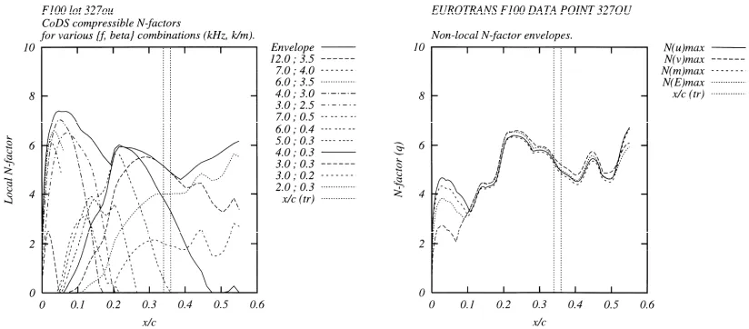
The F100 data point 327ou, illustrated in Figure 17, was selected for analysis during the EUROTRANS project because it qualified as a ‘pathological’ case, where transition occurred behind the peak N-factor and, in fact, in a region where all modes are stable according to linear analysis. Non-local theory has failed to change this situation, although the crossflow
N-factors towards the leading edge of the wing were reduced by 40%. These pathological cases require further attention from those developing more advanced transition prediction tools12 since most practical HLF designs would appear to fall into these categories. This does
3.8 Recent experiments and analysis
The analysis of the ELFIN II HLF tests has only recently been completed as part of the HYLDA project (1996 –1999). Other investigations carried out during that period include the HYLTEC project (1997 – 2000) and the Airbus Industrie 3E/LaTec project which saw the successful flight test of an HLF system on an A320 fin1. Some of these flights were funded by HYLDA, which has also funded a few additional tests on the ELFIN II tunnel model in order to maximise the return on investment. These more recent investigations and the associated analysis are now beginning to concentrate on more advanced aerodynamic issues, such as the correlating the N-factors of non-local stability methods, and practical experimentation with more realistic suction distributions than the ones required for N-factor correlation.
4 LINEAR STABILITY METHODS FOR DESIGN
Although much of the previous HLF design work was aimed at experiments which would provide useful data for correlating N-factors, recent activities within the HYLTEC project have studied the design of HLF systems which might be suitable for commercial application. These will be characterised by a greater emphasis on system simplicity and reduced mass flows and pumping requirements, and the changed design philosophy will place further demands on the use of linear stability and the eN technique.
Figure 19 illustrates the results from one of the early HYLTEC design exercises to retrofit an HLF system on the A310. N-factors are presented for a sample operating point M = 0.8,
Re = 30 million (based on the wing chord at 60% semi-span) and CL = 0.7: suction has been
applied up to 20% chord so as to suppress completely the growth of crossflow instabilities. This approach is similar to a number of experimental data points measured during the ELFIN II HLF tunnel campaign, but it expensive in terms of suction system complexity, power requirements and weight.
Figure 20 illustrates the opposite extreme, which is to reduce the suction rate until the crossflow N-factors are just below the critical value (taken to be 8 in this case). However we are now faced with the risk that this is now a pathological design where linear theory will fail. So a compromise solution is offered in Figure 21, which requires an intermediate amount of suction. This design was produced by constraining the maximum crossflow N-factor to be below a certain value. But what should this value be? Would it be different if a non-local analysis had been carried out? Both of these questions will impact upon the suction system specification and must therefore be answered by further research, using advanced methods, but which will allow the eN technique to be used with increased confidence for design.
Figure 19: local N-factors for an A310 retrofit design with crossflow growth completely suppressed.
Figure 20: local N-factors for an A310 retrofit design with crossflow growth controlled so that NCF < Ncrit.
[image:18.612.165.445.497.647.2]5 CONCLUSIONS AND RECOMMENDATIONS
Recent experimental work has allowed local, linear stability N-factor correlations to be derived, for the first time in Europe, for HLF systems. Following the analysis of the 3E/LaTeC A320 HLF fin flight tests a full range of critical N-factors will soon be known for both NLF and HLF applications and for tunnel or flight conditions.
A range of N-factor integration strategies have been evaluated during the analysis of these experiments. The envelope strategy, although it proved promising for NLF experiments, is not ideal for HLF design. The spanwise wavenumber strategy (C) is approximately equivalent to the wavelength strategy (B) for crossflow modes, and to the wave angle strategy (A) for Tollmien-Schlichting modes. The differing behaviour of crossflow and Tollmien-Schlichting modes may best be modelled by using a two-N-factor approach: a more rapid version of this approach considers only TS modes aligned with the external streamline (NTS) and stationary crossflow modes (NCF).
Correlated N-factors obtained with incompressible stability theory appear, thus far, to be more universal than N-factors obtained with compressible theory, which display some Reynolds number and Mach number dependence.
The use of non-local theory has demonstrated a significant effect on crossflow N-factors which warrants further, systematic correlation of these N-factors against experiment. If linear, non-local stability analysis improves the correlation between theory and experimental evidence then it is likely to be adopted for use in design.
Non-local, linear theory has not resolved the issue of pathological test cases. These cases are believed to display significant non-linear behaviour a long way upstream of transition, which invalidates one of the basic assumptions involved in the application of linear methods for transition prediction. The authors feel that the use of advanced non-linear transition prediction techniques can be used to provide guidance in the avoidance of pathological situations in the design of commercial HLF systems, but that linear stability theory is today's best tool for design purposes.
Database methods derived from linear theory can considerably accelerate the design process provided that they are validated appropriately against stability computations.
ACKNOWLEDGEMENTS
REFERENCES
[1] G. H. Schrauf, Evaluation of the A320 hybrid laminar fin experiment, European Congress on Computational Methods in Applied Science and Engineering (2000).
[2] J. Reneaux, J. Preist, J.C. Juillen, D. Arnal, Control of attachment line contamination, 2nd
European Forum on Laminar Flow Technology (1996), 8.3-8.16.
[3] D. Arnal, Boundary layer transition: predictions based on linear theory, AGARD R-793 (1994), paper 2.
[4] G. Schrauf, J. Perraud, D. Vitiello, F. Lam, Comparison of boundary layer transition
predictions using flight test data, J. Aircraft, 53 (1998), 891-897.
[5] G. Schrauf, J. Perraud, F. Lam, H.W. Stock, D. Vitiello, A. Abbas, Transition prediction
with linear stability theory – lessons learned from the ELFIN F100 flight demonstrator,
2nd European Forum on Laminar Flow Technology (1996), 8.58-8.71.
[6] M. Gaster, On the effects of boundary layer growth on flow stability, J. Fluid Mech., 66, 465-480.
[7] W.S. Saric, A.H. Nayfeh, Non-parallel stability of boundary layer flows, Phys. Fluids 18, (1975).
[8] T. Herbert, Parabolized stability equations, AGARD R-793 (1994), paper 4. [9] G. Schrauf, T. Herbert, G. Stuckert, Evaluation of transition in flight tests using
nonlinear PSE analysis, J. Aircraft, 33, (1996), 554-560.
[10] D. Arnal, EUROTRANS final report, EU 4th Framework Project no. BRPR-CT95-0069 (2000).
[11] L.M. Mack, Boundary layer stability theory, AGARD report R-709 (1984), paper no. 3. [12] G. Casalis, S. Hein, A. Hanifi, Non-linear transition prediction methods, European
Congress on Computational Methods in Applied Science and Engineering (2000). [13] D. Arnal, Private communication (1999).
[14] G. Schrauf, Transition prediction using different linear stability analysis strategies, AIAA Paper 94-1848, 12th AIAA Applied Aerodynamics Conference, Colorado Springs, USA (1994).