Measurement issues in the evaluation of projects in a
project portfolio
Alec Mortona
aDepartment of Management Science, Strathclyde Business School, University of Strathclyde, Glasgow G1 1XQ, United Kingdom. E-mail: [email protected]
Abstract
A common problem arising in many domains is how value the benefits of projects in a project portfolio. Recently, there has been some attention given to a decision analysis practice whereby analysts define a value function on some criterion by setting 0 as the value of the worst project. In particular, Clemen and Smith have argued this practice is not sound as it gives different results from the case where projects are ”priced out”, and makes a strong implicit assumption about the value of not doing a project. In this paper we underscore the criticism of this way of using value functions by showing it can lead to a rank reversal. We provide a measurement theoretic account of the phenomenon, showing that the problem arises from using evaluating projects on an interval scale (such as a value scale) whereas to guard against such rank reversals, benefits must be measured on at least a ratio scale. Seen from this perspective, we discuss how the solution proposed by Clemen and Smith, of explicitly reformulating the underlying optimisation problem to allow for explicitly non-zero values, addresses the issue, and explore in what sense it may be open to similar problems. In closing we discuss what lessons from practice may be drawn from this analysis, focussing on settings where the Clemen and Smith proposal may not be the most natural way of modelling.
Keywords: Decision analysis, Portfolio Decision Analysis, multicriteria decision analysis (MCDA)
1. Introduction
Supporting such decisions by evaluating projects and assessing the benefits of pos-sible portfolios as a function of the component projects represents a significant part of the professional work of many analysts. The application of decision analy-sis in such settings is often referred to as ”Portfolio Decision Analyanaly-sis”: Portfolio Decision Analysis seeks to provide frameworks for performing portfolio analysis in a way which allows a rigorous treatment of issues of value and uncertainty. Klein-muntz (2007) and Phillips and Bana e Costa (2007) have provided overviews of past work, and personal statements of what good practice looks like. The edited volume by Salo, Keisler and Morton (2011) provides a range of perspectives on theory and practice in this area.
A common practice in Portfolio Decision Analysis in a multicriteria setting is to define criterion-specific value functions by setting 0, the baseline for measurement, as the value of the worst item, as recommended by Phillips and Bana e Costa (2007, p 57) and implicitly recommended Kirkwood (1996); see for example Kirkwood’s example of Section 8.1 and the discussion in footnote 3 of Clemen and Smith (2009). These scores are then summed up across criteria to give an overall project score, and summed across the constituent projects to give an overall portfolio score. Clemen and Smith (2009) (henceforth, ”CS”) argue that it is not a sound approach to analysis as it gives different results from the case where projects are ”priced out”, and makes a strong implicit assumption about the value of not doing a project. As a solution, they advocate explicitly assigning project-specific value scores for not doing particular projects.
A number of scholars have sought to build on the work of CS. In particular, Liesi¨o and Punkka (2014) have explored how to elicit a suitable baseline value and also provide techniques for exploring sensitivity of the solutions recommended by a particular decision model to uncertainty about the appropriate baseline values. de Almeida et al. (2014) explore three consequences of rescaling the valuations of projects in a portfolio setting, which they dub the portfolio size effect, the baseline effect, and the issue of consistency across different aggregation sequences; and de Almeida and Vetschera (2012) explore a similar issue in the context of the PROMTETHEE multicriteria method.
capital budgeting in healthcare (Kleinmuntz and Kleinmuntz, 1999); an applica-tion to project selecapplica-tion in a telecommunicaapplica-tions company (Linstedt et al., 2008); and a military portfolio optimisation (Parnell et al., 2002). They comment that that this list is not exhaustive and they ”have found similar issues in many studies” (p 262). This author has had the same experience. For example, in the con-text of R&D prioritisation, Morcos (2008) recommends expressing scores ”along a value scale with intervals from 0 (least desirable) to 100 (most desirable)” (p 77). (Examination of the figures in this paper suggests that he departs from this rule in the case of one criterion, ”profitability” but adheres to it for the ”risk” and ”reliability” criteria.) Similarly Baltussen and Niessen (2006) present an illustra-tive example of multicriteria techniques to priority setting in healthcare (in which the task is to rank order projects with a view to deciding what subset of them to undertake) in which the zero has been set at the level of the least preferred project on three of four criteria (for the fourth criterion, ”severity of disease”, the projects are given between one and four stars, and the zero is set at one star). The reason for the pervasiveness of this practice seems to be that setting the zero at the level of the least preferred alternative is standard, unproblematic and uncontested ad-vice in the context where one is choosing a single item from a set. Many authors generalise this advice to the setting where the task is to choose multiple objects from a set.
In this paper we will study the setting of baselines from a measurement theo-retic point of view. Seen from this perspective, the issue is one which has surfaced in different forms in the literature over the years. In particular, Rao and Weiss (1986) provide a numerical exploration (in the context of a particular application) of the number of possible ways of ranking items in benefit/ cost order when the benefit scores of individual items are translated by a constant. Roberts (1990) provides an introduction to the theory of measurement and explores how it may be relevant in the context of combinatorial optimization problems: he observes that one can only be sure that the solution to a combinatorial optimization prob-lem will be invariant with respect to monotonically increasing transformations of its objective function coefficients when the optimizing algorithm uses only ordinal information about these coefficients (for example, a greedy algorithm).
and answer the following questions.
1. Can we get a clear view of what goes wrong when we use value functions to value projects multicriteria portfolio decision analysis?
2. What are the specific characteristics of value functions which give rise to this problem? Might this problem apply more generally when project benefits are assessed in some other way? In what way is this a specifically portfolio
problem?
3. Why does the solution proposed by CS ”work” to resolve this problem? Is the solution proposed by CS vulnerable to other similar and related problems? 4. How important is the separability of the rule for combining project benefit
values as overall portfolio benefits in this analysis? Do the results we obtain for this rule give insights into what should happen in a more general setting? 5. What, practically speaking, can we learn from this analysis about how to
perform better and more robust analysis?
The structure of the paper will be as follows. Section 2 will answer question 1. Section 3 will provide the analytic framework to answer the second and third groups of questions, which will be dealt with in Sections 4 and 5 respectively. Section 6 answers the fourth group of questions and Section 7 returns to the example of Section 2 to answer the question 5. Finally, Section 8 concludes.
2. Background
In this section we try to get a clear fix on the problem under consideration. To do so, consider the following example, which is smaller and thus hopefully gives a more direct insight into what is going on than that of CS. A government funded medical research institute has four research projects on the table. These projects will reduce mortality and contribute to scientific understanding, and the company cares both about the immediate medical and broader scientific benefits. Specifically, suppose that the projects have the profile of costs and benefits shown in Table 1.
Senior management’s value function over each of the two criteria is assessed as shown in Table 2, with values scores for each criterion referred to as Vmortality and
Reduced mortality Scientific impact Costs (£’000s)
a 6,000 lives saved Excellent 200
b 4,000 lives saved Good 100
c 4,000 lives saved Good 100
[image:5.595.147.456.104.175.2]d 3,000 lives saved Neutral 100
Table 1: Values and costs data
Vmortality Vscience Costs (£’000s)
a 1 1 200
b 1/3 1/2 100
c 1/3 1/2 100
d 0 0 100
Table 2: Values and costs data
Suppose we are seeking to maximize total benefits with a budget of £200,000 and we compute the values of portfolios as the values of the constituent projects. Irrespective of the weights applied, from the data of Table 2, the most attractive portfolio seems to be {a} which yields one unit on the scale of Vmortality, and one
unit of value on the scale of Vscience , whereas {b, c} yields only 2/3 on the scale
of Vmortality. At this point we might start to have doubts about the soundness of
this procedure, as {b, c} will save 8,000 people whereas {a} will save only 6,000, and so if saving lives is weighted heavily, {b, c} should appear more attractive.
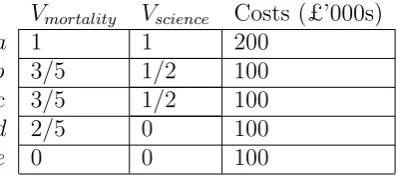
Such doubts are reinforced if we add a project e which saves 1,000 lives, has neutral scientific impact and costs £100,000 to the project list. In this case, we rescale the values to obtain the data shown in Table 3.
Vmortality Vscience Costs (£’000s)
a 1 1 200
b 3/5 1/2 100
c 3/5 1/2 100
d 2/5 0 100
[image:5.595.203.403.518.608.2]e 0 0 100
Table 3: Revised Values and costs
induced by the rescaling of the value function - a sure sign that we have done something problematic. Note that this phenomenon does not arise because of the linear transformation itself (as a monotonically increasing transformation this cannot change the ordering of projects within a criterion) but rather arises because of an interaction between the linear transformation and the use of an additive combination rule to compute overall portfolio scores. In any case, the rank reversal is a violation of the principle of Independence of Irrelevant Alternatives, according to which the preference for {a} over {b, c} or vice versa should not depend on whether portfolios including e are members of the choice set. Violation of this same principle has led many decision analysts to reject the Analytic Hierarchy Process as a method for supporting multicriteria choice (see e.g. Belton and Gear, 1983; Dyer, 1990; Salo and H¨am¨al¨ainen, 1997).
3. Derived measurement, consistency and invariance
In the technical part of this paper, we will address the following problem: suppose you have a set of benefit numbers, and the numbers are measured on a particular scale, and the numbers are combined in a particular way to give an overall portfolio value, what does the class of admissible transformations of the underlying scale have to be in order to avoid the sort of rank reversal problem which the example demonstrates? This problem embraces the question of what goes wrong with the decision analysis procedure discussed above, but casts it in a more general setting. Practising analysts – whether decision analysts or not – have numbers (such as benefit scores), and they do operations on these numbers (such as adding them up to come up with overall portfolio values), but are they doing this in an appropriate way?
if M1
V1 >
M2
V2. But can we be sure that if mass or volume had been measured using some different scale we would still be led to the same conclusion about relative densities?
In our approach we start with a (finite) set of objects A which are the objects of choice and a binary preference order%overA. When we say% is a preference relation we mean it is complete and transitive and so is representable by a real-valued function. The indifference relation ∼ and strict preference relation are defined in the usual way. We will be interested in the situation where we can compute a derived measurement which represents our preferences in the following sense.
Definition 1. A relation % on A is represented by the function v : A 7→ R iff a0 %a00 ⇔v(a0)≥v(a00) ∀a0, a00 ∈A.
The conditions for the existence of representing functions of various forms are well-known (Fishburn, 1970, Krantz et al, 1971).
We will suppose that the contents of A are vectors of decisions and mea-surements, formally that A = Rkn × {0,1}n for some positive integer n and
k ∈ {1,2}. The intended interpretation of the {0,1}n is that there are n
things which we could or could not do. The intended interpretation of the Rkn is that associated with each decision xi there is a vector of measurements
zi of dimensionality equal to k. Hence a generic element of A will be written as
(z, x) = ((z1, ..., zi, ..., zn),(x1, ..., xi, ..., xn)).
We restrict our focus in this paper to situations in which we are faced with binary decisions. In fact, often decisions can be thought of as polychotomous in the sense that one can choose different levels of different levels of investment (e.g. ”bronze”, ”silver” and ”gold”) in a project or area. Incorporating polychotomous investment decisions would not be difficult technically but this would render the notation more cumbersome, without providing additional insights.
professional disciplines such as accounting or epidemiology; or actual physical mea-surements (e.g. in the situation where the DM is interested in purchasing scrap metal and she may be able to weigh potential purchases). We highlight that we do not assume that these measurements are values assigned by a value function, although they could be.
The measurement system is such that a family of permissible transformations of the numbers are possible (for example revenues may be measured in British £
and we wish to convert them into e). We call this family F: the contents of F are functions f : Rkn 7→
Rkn. By a harmless abuse of notation we will also use f to denote a function which maps Rkn× {0,1}n into itself and is defined by
f(z, x) = (f(z), x), and F to be the set of such functions. Associated with each
f ∈ F (extended in this way) is a preference orderingR(f) on A. The indifference relation I(f) will be defined in the usual way. A set of functions and associated preference relations will be written hF,Ri.
Next, we define a notion of consistency.
Definition 2. A set of functions and associated relations hF,Ri is consistent with % iff a0 %a00 ⇔f(a0) R(f)f(a00)∀a0 , a00∈A,∀f ∈ F.
In the ensuing ”with%” will be understood and we will just write ”consistent”. Clearly this concept of consistency can be interpreted as ruling out rank re-versals when we perform some operation on the project benefit scores (such as rescaling them as we did in the example of the previous section).
We wish to distinguish consistency from another condition.
Definition 3. A relation % is F −invariant if a0 % a00 ⇔ f(a0) % f(a00)∀a0 , a00 ∈A,∀f ∈ F.
some particular threshold such we are indifferent to all levels of money above it. (We might find it hard to imagine what to do with the second billion eor £, but not with the second billion U.) Indeed, this is the difference between invariance and consistency: with consistency we are allowed to change the threshold when we rescale, with invariance not.
It is pretty clear that invariance is stronger than consistency, in the following sense:
Proposition 1. If % is F −invariant, and R(f) is defined by % ∀f ∈ F then
hF,Ri is consistent.
To give an example where we might have preferences which are consistent but not F −invariant, suppose that F = {f(z) = z−2} and % is defined by z0 % z00
iff −(z0 −2)2 ≥ −(z00 −2)2. Then 2 3 but f(3) = 1 0 = f(2), so % is not F −invariant. But if we define f(z0)R(f)f(z00) by −f(z0)2 ≥ −f(z00)2, then hF,Ri is consistent.
Obviously consistency is desirable from a normative point of view. Once we have converted £ into e or vice versa we should not find ourselves changing our minds about the attractiveness of our investments. However, it is also pretty weak by itself. In the ensuing we will have to supplement consistency by assuming the functions which represent%andR(f) have some particular functional form. This will make it possible to derive interesting results. Invariance, on the other hand, is a strong and normatively significant assumption, which can be used as the basis for representation theorems (see e.g. Sen, 1977).
4. One-part portfolio models
The setting for our first model is that we are confronted by n ≥ 2 ”projects” in which we can invest, and these projects have benefits if implemented. We have a measurement technology which maps the set of projects intoRn (i.e. k= 1) and an element in this space will be calledb = (b1, ..., bn). The intended interpretation
of such a point is that it corresponds to a set of projects where bi is delivered
through project i. In terms of our derived measurement framework, this vector b
properties do we require of the underlying measurement technology from which we obtain b?
The precise answer turns out to depend on the formula which is used to compute the overall portfolio value. The most natural formula is as follows.
Definition 4. If%on{0,1}n×
Rn is represented byP
i
bixi say it isrepresented by a one-part additive portfolio model.
The function P
i
bixi is the function recommended by Kirkwood (1996), and
which CS criticise as neglecting to explicitly draw attention to the value of not doing a project. The intended interpretation is that if a projectiis done (xi = 1)
then a benefit biis realized.
An important class of admissible transformations is as follows:
Definition 5. The set S of similarity transformations with common scal-ing factor is the set {f(·)|∃α∈R++,:f(b) = αb∀b ∈Rn}.
Obviously any similarity transformation of the underlying data will leave the preference ordering represented byP
i
bixi unchanged, but are there other
transfor-mations which have this property? The answer is no.
Proposition 2. If hF,Ri is consistent and %and R(f)are represented by a one-part additive portfolio model ∀f ∈ F, then F ⊆ S.
Proof. We develop the proof for the casen= 2: other cases are similar. We will write the representing portfolio model as v(·). Take an arbitrary f ∈ F. First observe that because both ((b,0),(1,0)) and ((b,0),(1,1)) have value b:
((b,0),(1,0))∼((b,0),(1,1)) (1)
Now, by consistency:
((f1(b), f2(0)),(1,0))I(f)((f1(b), f2(0)),(1,1)) (2)
Hence by representabilityv((f1(b), f2(0)),(1,0)) =v((f1(b), f2(0)),(1,1)) =⇒f1(b) =
solve the resulting equation by transforming both sides by ψ−1 to retrievef 1(b) =
f1(b) +f2(0)). By a parallel argument f1(0) = 0.
Now note that because % is represented by a one-part additive value function,
((b,0),(1,1))∼((0, b),(1,1)) (3)
Hence, by consistency:
((f1(b), f2(0)),(1,1))I(f)((f1(0), f2(b)),(1,1)) (4)
Hence, by representabilityf1(b)+f2(0) =f1(0)+f2(b) =⇒f1(b) =f2(b)∀b. Hence-forth write φ for both f1 and f2.
Now observe that:
((b1, b2),(1,1))∼((b1+b2,0),(1,1)) (5)
Hence, by consistency again:
((φ(b1), φ(b2)),(1,1))I(f)((φ(b1+b2), φ(0)),(1,1)) (6)
From which we can conclude thatφ(b1) +φ(b2) = φ(b1+b2), which is a Cauchy functional equation. As is well-known (Acz´el, 2006), the only solution to this equation is φ(b) =αb. Hence the result is proved.
Recall that an absolute scale is one where no transformations are permissible; a ratio scale is one where similarity transformations (ie multiplication by a scaling factor) are permissible; and an interval scale is one where affine transformations (multiplication by a scaling factor and addition of a positive constant) are permis-sible. So the implication of Proposition 2 is that if the project benefit scores are measured on an absolute scale, no rank reversal is possible; if they are measured on a ratio scale, no rank reversal is possible; but if they are measured on (for ex-ample) an interval scale, then a rank reversal can occur, indicating that we have a problem. Value functions are generally taken to be measured on an interval scale, and it is this which justifies the rescaling as the option set changes, which in turn gives rise to the rank reversal described in Section 2.
consistent transformations (ie transformations which do not induce a rank rever-sal) is dependent on the choice of portfolio model. For example, if the portfolio model is max
i {bixi} then F can contain any strictly increasing function without
fear of inducing an inconsistency (the best portfolios are those which contain the best project, and no strictly increasing transformation will change the ranking of the projects), and so rescalings are unproblematic, as long as the benefits of all projects are rescaled by the same amount. To take another example, if the portfo-lio model is Π
ibixi thenF can be contained in the following set without introducing
an inconsistency:
Definition 6. The setW of weighted power transformations is the set{f(·)|∃αi ∈
R++,∃p∈R++:fi(r) = αirp ∀r ∈R}.
In other words, the range of transformations which may feature in F without inducing an inconsistency is enlarged - but nevertheless, measuring benefits on interval scales which permit a change in zero point (for example, value functions) is still problematic even with this choice of one-part additive portfolio model.
5. Two-part portfolio models
In the second formalisation we have n ≥ 2 ”sectors” in which we can invest or not. Investing in a sector leads to different outcomes than if we had not invested. Sectors could be locations, or diseases, or physical installations, such as roads or flood defences; if one is planning flood defences, the decision could be to upgrade from sand defences to concrete. We have a measurement technology which measures the outcomes associated with investing and not investing, i.e now our measurement technology produces 2n measurements (k = 2). Specifically, associated with each sectoriwe have a measurement of the outcomezi in the case
where we invest and zi in the case where we do not invest. Write zi = (zi, zi).
We use a model of the form P
i
zixi +zi(1−xi)
as a representing portfolio function for these preferences (this is the model which is recommended in CS as equation (3)). It will be noted that when this modelP
i
zixi+zi(1−xi)
is used the conclusions of the previous section do not hold: in particular, a transformation of the formfi(zi) =zi+βapplied to bothziandzi will obviously leave the ranking
of solutions induced by this portfolio model unchanged.
Definition 7. If% is represented by P
i
zixi+zi(1−xi)
say it is represented by a two-part additive portfolio model.
We define the following set of transformations. Note that α is a scalar and β
is a vector.
Definition 8. The setA of affine transformations with a common scaling factor is the set {f(·)|∃α ∈R++,∃β ∈Rn:f(z) = αz+β∀z ∈Rn}.
As in the previous section, the transformations in the designated set are the only transformations to leave the preference ordering unchanged.
Proposition 3. If hF,Ri is consistent and % andR(f)are represented by a two-part additive portfolio model ∀f ∈ F, then F ⊆ A.
Proof. Take an arbitraryf ∈ F. Observe that the indifference ((z,0),(0,0),(1,0))∼ ((0,0),(z,0)(0,1)) follows from representability. Hence from consistency:
(((f1(z), f1(0)),(f2(0), f2(0))),(1,0))I(f) (((f1(0), f1(0)),(f2(z), f2(0))),(0,1))) (7) from this it follows that:
f1(z) +f2(0) =f1(0) +f2(z) (8)
or in other words, f1(z) and f2(z) differ only in a constant term. Call this term κ and write f2(z) = f1(z)+κ.
Now observe that (((z1,0),(z2,0)),(1,1)) ∼ (((z1 + z2,0),(0,0)),(1,1)) and hence:
(((f1(z1), f1(0)),(f1(z2) +κ, f1(0) +κ)),(1,1))I(f)
Because the κs cancel, it follows that:
f1(z1) +f1(z2) =f1(z1+z2) +f1(0) (10)
This is equivalent to:
f1(z1)−f1(0) +f1(z2)−f1(0) =f1(z1+z2)−f1(0) (11)
Hence we can define γ(z) = f1(z)−f1(0) and obtain the following functional equation:
γ(z1) +γ(z2) =γ(z1+z2) (12) This is the Cauchy equation again, so γ(z) = αz. Write β1 = f1(0) and
β2 =f1(0) +κ and we have an affine transformation with common scaling factor as claimed.
Hence, for these two part functions, using value functions (or other measure-ment technologies) which provide interval valued measuremeasure-ments, does not represent a threat to consistency and place us at risk of inducing a rank reversal.
Does this mean that we can disregard nature of the scales on which the out-comes are measured when using such two-part models? Absolutely not! Consider the following example.
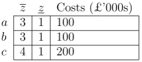
[image:14.595.232.371.475.536.2]Example 1. Suppose outcomes are measured on an ordinal scale, and portfolios are evaluated by a two-part additive model. Consider the following data shown in Table 4 for some evaluation problem.
z z Costs (£’000s)
a 3 1 100
b 3 1 100
c 4 1 200
Table 4: Outcomes and cost data
Suppose we have a budget of £200,000. The optimal choice is portfolio {a, b}
because the value of the model P
i
zixi+ P i
zi(1−xi)is 3 + 3 + 1 = 7 whereas if we
choose {c} we obtain 1 + 1 + 4 = 6. However, if a transformation f(z) = z3 is
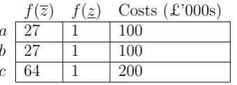
applied to the zs andzs (since all strictly increasing transformations of an ordinal scale are permissible), then the data become as shown in Table 5.
Now if we apply the formula P
f(
i
zi)xi+ Pf( i
zi)(1−xi) {a, b} is associated
f(z) f(z) Costs (£’000s)
a 27 1 100
b 27 1 100
[image:15.595.218.389.100.161.2]c 64 1 200
Table 5: Transformed outcome and costs data
Comparing Proposition 2 and Proposition 3 gives us some insight into why us-ing value functions (or indeed any measurement technology which produces num-bers measured on an interval scale) to evaluate benefits is problematic in the case of a one-part additive portfolio model but non-problematic in the case of a two-part additive portfolio model. However, Example 1 shows us that we would experience a problem exactly analogous to the problem of Section 2 when using a two part function additive portfolio model if we were to use a technology which produced measurements on an ordinal scale to measure benefits.
Moreover, our positive conclusion that it is safe to choose an interval scale when using a two-part portfolio model is not necessarily good if the model in question does not have an additive form - for example a model with the multiplicative form Π
i zixi+zi(1−xi)
. Consider the following example.
Example 2. We are seeking to build a small research team, and we need a math-ematician (m) and a programmer (p). We have people with both these skills in house, but we have some funds and can hire either a better m or a better p (but not both). We rate both existing and potential new hire ms and ps on a zero to 100 scale as follows, with z denoting the score for the new hire and z denoting the score for the existing staff, as in Table 6.
z z
m 48 30
p 60 40
Table 6: Original staff evaluations
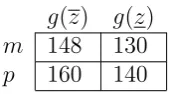
[image:15.595.267.333.526.570.2]thought - these are skilled professionals, so surely we should start the scale at 100 instead of zero and go up to 200? We thus transform our scores by the function g(z) =z+ 100. This gives us new scores as shown in Table 7.
g(z) g(z)
m 148 130
[image:16.595.258.343.157.204.2]p 160 140
Table 7: Transformed staff evaluations
Now we recompute the portfolio scores. This time, the portfolio containing the new m and the existing p has a total score of 148×140 = 20720 and the portfolio containing the existing m and new p has a total score of 130×160 = 20800, so it seems now we should hire the new programmer instead.
In this case we have performed an affine transformation of the underlying scale – quite permissible if the scale is indeed an interval scale – and have obtained a rank reversal, even though we are using a two-part model. This is not a coincidence, and in fact it can be shown (using the same line of reasoning as that of Propositions 2 and 3) that in the case of a two-part multiplicative model the only transformations of the underlying scales which preserve consistency are those in the set W, as introduced in the last section.
6. Beyond separable models
So far in this paper, we have identified admissible transformations of underlying data which preserve particular value models. However, a possible objection to this analysis is that we have so far focussed exclusively on additive and other separable value models. This is a significant restriction in a portfolio context as often there will be interactions between decisions about particular projects or particular sectors. For example, the value of investing in secondary care facilities for people suffering from stroke or advanced kidney disease may depend on whether one has also invested in preventive activity for these conditions; to the extent that one has not invested in prevention, one can expect secondary care facilities to have higher utilization and thus add more value.
Administration where particular profiles of maintenance decisions are mapped into a descriptive system which captures the distribution of the various elements of the road infrastructure across a number of quality classes. This in turn is mapped by a multiattribute value function with four criteria representing road safety, asset value preservation, customer satisfaction and environmental aspects, into a value score. In our terms, one can think of this formal apparatus as a device for mapping a profile of decisions into an outcome space, with non-zero outcomes associated both with choosing both with ”doing” and ”not doing” a particular piece of maintenance. Such a model ”feels like” a two-part model but the outcome values need not combine additively over sectors (for example, in the Mild and Salo (2009) model, as there is a Markov chain which governs the degradation of the roads over time, a maintenance action in one period may interact with a maintenance action in a subsequent period).
Is there anything we can say, then, about these situations where we do not have separability between decisions? It turns out there is. To see what may be generalizable to this more complex environment, make the following definition:
Definition 9. The set T of translations is the set {f(·)|∃β ∈Rn,:f(b) =b+β
∀b∈Rn}.
One of the striking feature of the previous section has been that the project value models of Section 4 are not consistent with respect to sets of data transfor-mations containingT (even the portfolio model max
i {bixi}requires us to transform
each project score by the same monotonic function), whereas the sector value mod-els of Section 5 may be (for example the class of consistent transformations of the two part additive model is a superset of T).
To see how this insight applies in a more general setting, in this section, rather than studying relations represented by particular functions, we study a property imposed on the relation itself directly. We continue to suppose that% is a prefer-ence ordering but no longer suppose that it has an explicit representation through a specific portfolio model. Instead we will be interested in the following property.
Definition 10 (PC). A preference relation%overA=Rkn×{0,1}n(k ∈ {1,2})
(z00,0n)∀z0, z00 ∈
Rkn where 0kn,0n are the zero vectors of dimensionality kn and
n respectively, and 1n is a vector of ones of dimensionality n.
Thus, part (i) of one-part coherence captures the idea that a zero on the benefit scale has the meaning that one is indifferent between doing a project and not doing it. Part (ii) says that if one does not do any project, it does not matter how much benefit would have been realized had one done some.
It is interesting to compare with this what one may think of as the essential features of the two-part representation. Consider the following axiom.
Definition 11 (SC). A preference relation % over A = R2n × {0,1}n will be
called two-part coherent if
((z1, z1), ...,(zi, zi), ...,(zn, zn)),(x1, ...,1, ..., xn))
∼ ((z1, z1), ...,(zi, zi), ...,(zn, zn)),(x1, ...,0, ..., xn))
∀i ∈ {1, ..., n}, ∀(z1, z1), ...,(zi−1, zi−1),(zi+1, zi+1), ...,(zn, zn)) ∈ R2(n
−1) and
∀zi, zi, zi ∈R.
This axiom captures the idea that whether one obtains zi from choosing 1 or from choosing 0 is a matter of indifference: it is the same zi in either case.
We also need a very mild axiom.
Definition 12. A preference relation% overA=Rkn× {0,1}n will be said to be essential if ∃z0, z00∈Rkn : (z0,1n)(z00,1n).
To see that one-part and two-part coherence are very different ideas, consider the following result.
Proposition 4. No preference relation % over A = R2n × {0,1}n can be both
one-part coherent, two-part coherent and essential.
Proof. For conciseness, writez = [(zi, zi)]. Choosez
0 = [(z0 i, z
0
i)], z
00 = [(z00 i, z
00
i)] :
(z0,1n)(z00,1n). By part (ii) of PC, ([(z0
i, z
0 i)],0
n)∼([(z00
i, z
00 i)],0
n) ∀z0
i, z
00
i ∈R.
By SC, ([(zi0, z0i)],0n)∼([(z0i, z0i)],1n) and ([(zi00, z00i)],0n)∼([(z00i, z00i)],1n). From the transitivity of indifference, we can conclude (z0,1n) = ([(z0
i, z 0
i)],1n)∼([(z
00 i, z
00
i)],1n) =
We are able to prove an impossibility theorem for one-part coherence.
Theorem 3. For all preference relations % over A = Rn × {0,1}n, if hF,Ri
is consistent and % and R(f) are essential and one-part coherent ∀f ∈ F then
T *F.
Proof. Suppose T ⊆ F and consider z0 and z00 distinct such that (z0,1n) (z00,1n). Now apply the transformation f
i(zi) = zi − z0i ∀i to z
0 to obtain:
((f1(z1), ..., fn(zn)),1
n) = (0n,1n). By PC part (i), (0n,1n)I(f)(0n,0n) and
so by consistency, (z0,1n) ∼ (z0,0n). By parallel reasoning, (z00,1n) ∼ (z00,0n).
Hence by transitivity of strict preference, (z0,0n) (z00,0n)). But this is a
con-tradiction toPC part (ii).
Thus, it is not possible to measure the benefit values in any one-part model on a scale which permits arbitrary translation without exposing oneself to the possibility of rank reversal. Contrast this with the main result (Proposition 3) which shows that it is possible to measure the benefit values in two-part models on such a scale with no such risk.
The non-permissibility of translation in portfolio models which represent project-wise coherent preferences is important for practical purposes, in that it shows that the reason for the sorts of pathologies by the one-part model exhibited in Section 2 do not arise because of some quirk of the additive form: in fact they are much more general. Moreover, as will be apparent in the next section, the idea of one-part coherence gives actual operational guidance into how a natural baseline for mea-surement can be fixed to avoid the sorts of rank reversal pathologies documented in Section 2.
7. Implications for practice
In this section, we return to the fundamental question: how should practising analysts model problems like that of Section 2? CS are proponents of the additive two-part model P
i
zixi+
P
i
zi(1−xi) as a way of dealing with the baseline setting
where it is more natural to use one-part models. We illustrate our argument by revisiting the case where a government funded medical research institute wishes to select a portfolio of projects without spending in excess of a budget. The aim is to develop medications for a potentially lethal disease (let us say diabetes). One of the criteria for evaluation is impact on mortality. We argue that it is more natural to use a one-part model rather than a two-part model in this case.
The principal reason is that a significant attractive feature of the one-part model P
i
bixi , is that one does not have to explicitly to identify the outcomes in
terms of how many people die from diabetes associated with not doing a project, which may be contentious and not decision relevant. For example, knowing the precise extent of diabetes in a population (as long as it is agreed that there is ”a lot”) may not be relevant to decisions between a number of ”small” projects to redress diabetes, since only once the projects become sufficiently large that one may run out of people to treat does the scale of the underlying health problem become an issue. This is a real concern in economically underdeveloped countries with poor systems of public health surveillance and death registration, estimating how many people in the general population have a given disease and how many people die from that disease to a high level of accuracy is for all practical purposes impossible.
To illustrate how this might work, let us return to the example of Section 2. If one evaluates ”lives saved” relative to this ”zero projects implemented”/ ”zero lives saved” baseline as the zero of the measurement scale, takes the level of the most beneficial project - ”6,000 lives saved”- as the unit and assumes a linear value function, referring back to the original column of Table 1, one obtains value scores of 1, 2/3, 2/3 and 1/2 for the different projects respectively. Note that this value measurement system does not give unique measurements: if we add an extra project which saves 10,000 lives to the option set, we have to rescale the value scores to get 3/5, 2/5, 2/5 and 3/10 fora,b, c, drespectively, but this simply involves multiplying the original value scores by a common constant (a similarity transformation), so the ranking of portfolios we obtain from summing up these value scores is unaffected. Proposition 2 tells us that whenever we want to add up value scores in this way, we can only be sure that our measurement system will not induce a rank reversal of portfolios if the permissible score transformation are similarity transformations. This is the reason that the original procedure of Section 2 gets us into difficulties. Now, because we have chosen a baseline which is independent of the choice set and does not change when we add projects, we no longer have to worry about rank reversals.
As a matter of fact, this approach of setting a so-called ”do nothing” baseline has been used widely in the multicriteria context in practice, in papers as early as e.g. Bana e Costa et al. (1999, 2002). Indeed, this is what is done in the case study presented in Phillips and Bana e Costa (2007) (despite these authors’ advice to set the 0 at the level of the least preferred option). Hence we see the contribution of this paper as being in part to justify the procedure of these authors, which recognises the problem identified by CS but approaches its solution in a different and to our way of thinking more natural manner.
Hence, while we recognise the issue which CS raise, our view is that the solution that they suggest - using P
i
zixi+
P
i
zi(1−xi) - is not always the most natural
modelling solution. It is perfectly possible to continue to describe problems using the additive one-part model P
i
bixi as long as one takes care the the coefficients
for measurement which is independent of the set of projects being considered for inclusion in the project portfolio. As part of the theoretic contribution of this paper, our ”one-part coherence” axiom of Section 6 can give insight into the most appropriate way to identify this baseline.
8. Conclusion
This paper has studied the issue of the choice of measurement scales to measure project benefits in multicriteria portfolio decision analysis using a derived measure-ment frame, motivated by an issue in MCDA practice. The distinctive feature of our frame here has been that we suppose that we have some measurements, and some way of combining them, and wish the resulting derived measurement to have certain consistency properties. We then ask what properties the underlying tech-nology which has produced our measurements would have to have (bearing in mind that these measurements may be from judgemental elicitation, from the use of the techniques of professional disciplines such as accounting or epidemiology, or from some actual physical measurement system).
We relate our conclusions back to our motivating questions as follows:
1. Can we get a clear view of what goes wrong when we use value functions to value projects multicriteria portfolio decision analysis? We provide a small toy example showing that, in an environment where additive functions are used to combine project values, rescaling value functions by changing the baseline of measurement can lead to rank reversals between portfolios. 2. What are the specific characteristics of value functions which give rise to this
problem? Might this problem apply more generally when project benefits are
assessed in some other way? In what way is this a specifically portfolio
scale for the measurement of benefits leads to a rank reversal problem de-pends on the nature of the portfolio model used to combine benefit scores - for example one could safely use interval scales for the measurement of benefit functions if a max function was use to transform value scores. 3. Why does the solution proposed by CS ”work” to resolve this problem? Is the
solution proposed by CS vulnerable to other similar and related problems?
In the alternative ”two-part” additive model which CS propose, the class of transformations by which the benefits can be rescaled without inducing a rank reversal is the class of affine transformations, so using value functions is unproblematic in this context. But rank reversals can still be induced in the two two-part additive models if benefits are assessed on other scale types (e.g. ordinal) and rescaling project values by an affine transformation is still a problem if a two-part multiplicative model is used – so two part models are not immune to rank reversal problems if one is careless about the nature of the scale on which the underlying benefits are measured.
4. How important is the separability of the rule for combining project benefit values as overall portfolio benefits in this analysis? Do the results we obtain
for this rule give insights into what should happen in a more general setting?
Even in the case of non-separable portfolio models, there is a clear difference between the one- and two-part models, in that the one-part models can never be used with benefit scores assessed on scales which allow arbitrary scale translation, whereas this is unproblematic in the case of the two-part additive model.
Our philosophy in writing this paper has been that mistakes (like the mistake highlighted by CS) are worth studying in some detail as a close understanding of how one has gone wrong in the past can ensure that one learns the right lessons and does not overlearn (for example it is not the case that it is always wrong to use interval scales to assess benefit values when using one-part models), and avoid making similar mistakes in the future (for example using interval scales in the setting where one has two-part multiplicative models). We hope that the discussion and findings in this paper will help researchers and practitioners draw appropriate conclusions about how to assess benefits in portfolio settings.
Acknowledgements. A great debt is owed to Carlos Bana e Costa who
References
1. Acz´el, J. (2006). Lectures on functional equations. Mineola, NY: Dover. 2. Baltussen, R. and Niessen, L. (2006) Priority setting of health interventions:
the need for multi-criteria decision analysis. Cost-effectiveness and resource allocation, 4(14).
3. Bana e Costa, C., da Costa-Lobo, M. L., Ramos, I. A., & Vansnick, J.-C. (2002). Multicriteria approach for strategic planning: the case of Barcelos. In D. Bouyssou, E. Jacquet-Lagr`eze, P. Perny, R. S lowinsky, D. Vander-pooten & P. Vincke (Eds.), Aiding decisions with multiple criteria: essays in honour of Bernard Roy: Kluwer.
4. Bana e Costa, C. A., Ensslin, L., Correa, E. C., & Vansnick, J.-C. (1999). Decision Support Systems in Action: Integrated Application in a MultiCri-teria Decision Process. European Journal of Operational Research, 113(2), 315-335.
5. Belton, V., & Gear, T. (1983). On a Short-Coming of Saaty Method of Analytic Hierarchies. Omega-International Journal of Management Science, 11(3), 228-230.
6. Belton, V., & Stewart, T. J. (2002). Multiple Criteria Decision Analysis: an integrated approach. Boston, MA: Kluwer.
7. Clemen, R. T., & Smith, J. E. (2009). On the choice of baselines in mul-tiattribute portfolio analysis: a cautionary note. Decision Analysis, 6(4), 156-262.
8. de Almeida, A.T., Vetschera, R. (2012). A note on scale transformations in the PROMETHEE V method. European Journal of Operational Research, 219, 198-200.
9. de Almeida, A.T., Vetschera, R., Almeida J. A. (2014). Scaling Issues in Additive Multicriteria Portfolio Analysis. In F. Dargam, J. E. Hern´andez; P. Zarat´e. S. Liu, R. Ribeiro, B. Delibasic, J. Papathanasiou (Eds.),Decision Support Systems III - Impact of Decision Support Systems for Global Envi-ronments. LNBIP 184 (Lecture Notes in Business Information Processing): Springer. 131-140.
11. Fishburn, P. C. (1970). Utility theory for decision making. Chichester: Wiley. 12. Golabi, K., Kirkwood, C. W., & Sicherman, A. (1981). Selecting a portfolio of solar energy projects using multiattribute preference theory. Management Science, 27, 174-189.
13. Kirkwood, C. (1996). Strategic Decision Making: Multiobjective Decision Analysis with Spreadsheets. Belmont, CA: Duxbury.
14. Kleinmuntz, C. E., Kleinmuntz, D. N. (1999). A strategic approach to al-locating capital in health-care organizations. Healthcare Financial Manage-ment 53(4) 52–58.
15. Kleinmuntz, D. N. (2007). Resource allocation decisions. In W. Edwards, R. F. Miles & D. von Winterfeldt (Eds.), Advances in decision analysis (pp. 400-418). Cambridge: CUP.
16. Krantz, D. H., Luce, R. D., Suppes, P., & Tversky, A. (1971). Foundations of Measurement Vol 1. New York: Academic Press.
17. Liesi¨o, J. , Punkka, A. (2014). Baseline value specification and sensitivity analysis in multiattribute project portfolio selection. European Journal of Operational Research 237, 946–956.
18. Lindstedt, M., Liesi¨o, J. , Salo, A. (2008). Participatory development of a strategic product portfolio in a telecommunication company. International Journal of Technology Management, 42(3), 250–266.
19. Mild, P., & Salo, A. (2009). Combining a Multiattribute Value Function with an Optimization Model: An Application to Dynamic Resource Allocation for Infrastructure Maintenance. Decision Analysis, 6(3), 139–152.
20. Milnor, J. (1954). Games against nature. In R. M. Thrall, C. M. Coombs & R. L. Davis (Eds.), Decision Processes. New York: Wiley.
21. Morcos, M. S. (2008). Modelling resource allocation of R&D project port-folios using a multi-criteria decision-making methodology. International Journal of Quality and Reliability Management, 25(1), 72-86.
22. Morton, A. (2010). Bridging the gap: health equality and the deficit framing of health. Health Economics, 19(12), 1497-1501.
24. Parnell, G. S., Bennett, G. E. , Engelbrecht, J. A., Szafranski, R. (2002). Improving resource allocation within the National Reconnaissance Office.
Interfaces, 32(3), 77–90.
25. Phillips, L. D., & Bana e Costa, C. (2007). Transparent prioritisation, bud-geting and resource allocation with multi-criteria decision analysis and deci-sion conferencing. Annals of Operations Research, 154(1), 51-68.
26. Rao, V. R., & Weiss, E. N. (1986). On Resource-Allocation Problems with Interval-Scale Coefficients. Journal of the Operational Research Society, 37(6), 631-635.
27. Roberts, F. S. (1990). Meaningfulness of conclusions from combinatorial optimization. Discrete Applied Mathematics, 29(2-3), 221-241.
28. Salo, A. A., & H¨am¨al¨ainen, R. P. (1997). On the measurement of prefer-ences in the analytic hierarchy process. Journal of Multi-Criteria Decision Analysis, 6(6), 309-319.
29. Salo, A. A. , Keisler, J., Morton, A., eds. (2011). Portfolio Decision Anal-ysis: Methods for improved resource allocation. New York: Springer.
30. Sen, A. (1977). On Weights and Measures - Informational Constraints in Social-Welfare Analysis. Econometrica, 45(7), 1539-1572.
31. Suppes, P., & Zinnes, J. L. (1963). Basic Measurement Theory. In R. D. Luce, R. R. Bush & E. Galanter (Eds.), Handbook of Mathematical Psy-chology. New York: Wiley.