Dynamic and structural performances of a new sailcraft concept for interplanetary missions

(1)

Research Article

Dynamic and Structural Performances of a New Sailcraft

Concept for Interplanetary Missions

Alessandro Peloni,

1

Daniele Barbera,

2

Susanna Laurenzi,

3

and Christian Circi

3 1_{School of Engineering, University of Glasgow, Glasgow G12 8QQ, UK}

2_{Faculty of Engineering, University of Strathclyde, Glasgow G1 1XW, UK}

3_{Department of Astronautic, Electrical and Energy Engineering, Sapienza University of Rome, Via Salaria 851, 00138 Rome, Italy} Correspondence should be addressed to Christian Circi; [email protected]

Received 6 February 2015; Accepted 11 June 2015

Academic Editor: Manuel Lozano

Copyright © 2015 Alessandro Peloni et al. This is an open access article distributed under the Creative Commons Attribution License, which permits unrestricted use, distribution, and reproduction in any medium, provided the original work is properly cited.

Typical square solar-sail design is characterised by a central hub with four-quadrant sails, conferring to the spacecraft the classical X-configuration. One of the critical aspects related to this architecture is due to the large deformations of both membrane and booms, which leads to a reduction of the performance of the sailcraft in terms of thrust efficiency. As a consequence, stiffer sail architecture would be desirable, taking into account that the rigidity of the system strongly affects the orbital dynamics. In this paper, we propose a new solar-sail architecture, which is more rigid than the classical X-configuration. Among the main pros and cons that the proposed configuration presents, this paper aims to show the general concept, investigating the performances from the perspectives of both structural response and attitude control. Membrane deformations, structural offset, and sail vibration frequencies are determined through finite element method, adopting a variable pretensioning scheme. In order to evaluate the manoeuvring performances of this new solar-sail concept, a 35-degree manoeuvre is studied using a feedforward and feedback controller.

1. Introduction

Solar sailing is a promising technology, which allows plan-ning missions otherwise impracticable using traditional propulsion systems. Therefore, the solar-sailing concept opens up new avenues for scientific discoveries in many fields of astronautic science, from materials engineering to flight dynamics [1–5]. Due to the continuous and propellant-free thrust, solar sails are mainly studied for orbits with high ΔV requirements, such as Earth Pole-sitter orbits [6– 8], orbits at the Earth-Moon libration points [9,10], or new kinds of orbits around the Earth, as the Taranis orbits [11, 12]. Attitude control and optimal steering laws to improve sailcraft performances have recently been studied in several works as well [13–17].

Sailcrafts have a very large and complex structure, typi-cally formed by four petal membranes, which are tensioned to form the square shape using deployable ultrathin com-posite booms [18–22]. Alternative methods for deploying

and tensioning the membrane were also investigated and tested, such as in the case of IKAROS, the first-launched solar-sail demonstrator [23]. In that case, the four trapezoidal membranes are linked together using spaced strips, which facilitate the folding of the membrane. The solar sail was then deployed and kept extended in a flat shape by the centrifugal force due to the spin of the sailcraft itself. In all mentioned cases, even in the IKAROS demonstrator that did not use booms, the solar sail is visually and physically divided into four membranes and a central hub, which gives the typical X-configuration to the spacecraft.

This work proposes a new approach to the solar-sail design with a different kind of configuration, in which the classical central bus is divided into four hubs displaced at the corners of the square sail. With this configuration, the sail tensioning can be controlled more easily and the tensioning motors, if any, can be directly placed on the hubs. The membrane tensioning is an important topic, due to the formation of wrinkles or bubbles born from the

(2)

2 4 3 1

2

4 3

1

Opening sequence

Sail membrane

[image:2.600.53.291.73.165.2]

Stowed sailcraft Deployed sailcraft

Figure 1: Sailcraft opening sequence.

tensioning or thermal load. This feature is crucial for the masking, shadowing, and thermal issue that may afflict sail performances. From an attitude control point of view, this configuration allows the attitude control thrusters, if any, to be directly mounted on the hubs rather than on the top of a flexible boom. Therefore, the thruster is more likely to be in the nominal position. This feature and the stiffer nature of the architecture itself entail the sail being flatter than in the X-configuration. Moreover, this type of architecture can be considered as the unit part of a bigger modular solar sail. On the other hand, the dislocated nature of this configuration increases the moments of inertia of the sailcraft, with a possible decrease of the attitude control efficiency.

This paper investigates the structural and the dynamics performances of the proposed novel configuration of the solar sail. To compare both the structural and the attitude control performances of this new architecture with those available in literature, a 40 m side sail has been considered for the study.

The paper is organised as follows: the new sail config-uration is presented inSection 2; a finite element model is reported in Section 3for the evaluation of maximum out-of-plane displacement, vibration frequencies, and calculation of the offset between the centre of mass and the centre of pressure. The offset value is used inSection 4to investigate the solar-sail attitude control performances for a 35-degree deep space manoeuvre.

2. Solar-Sail Concept Configuration

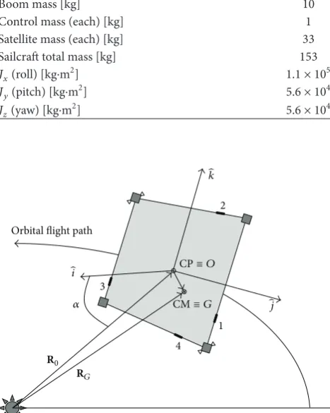
The solar-sail geometry proposed in this study is a classical square, with the booms on the perimeter of the membrane and the mass of the satellite divided into four parts, collocated on the square’s corners and joined at the booms’ end. The opening sequence from the closed-shape launch configura-tion to the deployed one (Figure 1) is helped by the strain energy stored in the booms. The deployment velocity is a function of the booms’ shapes and the parameters of the deployment mechanism [24,25].

Table 1shows the main sailcraft’s characteristics, accord-ing to [26], whileFigure 2shows the solar-sail reference frame taken into account. The sail mass inTable 1is computed by considering the same film as in [26], in which the 1200 m2 sail has a mass of 6 kg. The boom mass is calculated in the same way. The origin of the body reference frame is set on the geometric centre, roll axis(̂𝑖)is perpendicular to the sail plane, and pitch(̂𝑗)and yaw(̂𝑘)axes are the transverse axes

Table 1: Sailcraft properties.

Sail side [m] 40

Sail area [m2] 1600

Sail mass [kg] 8

Boom mass [kg] 10

Control mass (each) [kg] 1

Satellite mass (each) [kg] 33

Sailcraft total mass [kg] 153

𝐽𝑥(roll) [kg⋅m2] 1.1×105

𝐽_𝑦(pitch) [kg⋅m2_] ₅_.₆_×₁₀4

𝐽𝑧(yaw) [kg⋅m2] 5.6×104

1 2

3

4 Orbital flight path

̂k

̂i

̂j 𝛼

R0 RG

CP≡ O

[image:2.600.310.553.87.217.2]

CM≡ G

Figure 2: Solar sail in interplanetary trajectory.

parallel to the booms.𝛼is the cone angle between the Sun-line direction and the roll axis,R𝐺is the position vector of centre

[image:2.600.312.546.131.424.2]

(3)

3. Structural Analysis

In this study, we performed nonlinear static analysis, based on Finite Element Method (FEM), adopting the commercial code ABAQUS. The aims of this investigation were the deter-mination of the membrane out-of-plane deflections caused by the solar pressure, the natural modes of the structures, and the disturbing momentum due to offset between the CP and the origin of the body reference frame, varying the tension applied to the corner of the solar sail. Particular attention was paid when calculating the offset value, which will be used in the dynamics analysis to evaluate the manoeuvring performances of the novel square configuration.

The solar sail is a large thin membrane structure with the bending stiffness negligible compared to the in-plane stiffness; thus the membrane cannot carry compressive stress. The flat square shape is controlled by the use of tensioning loads applied at the membrane corners. When the tensioned membrane is exposed to the solar pressure, out-of-plane large deformations occur and wrinkles can be formed with the origin sets in the corner membrane. The numerical simulation of the wrinkles’ formation is still an open issue, since the wrinkles alter the membrane shape and thus the final performances of the solar sail. Authors investigated numerically the wrinkles’ amplitude tension load depen-dency, considering the membrane truncated at the corners in order to avoid stress concentrations in those locations [30]. However, the analysis of the wrinkles’ behaviour is not the focus of this current study and will be analysed in a separate work.

In this study, we investigate the structural response of a flat, square, thin-film membrane tensioned at the corners. Considering the FEM model, the easiest way of pretensioning the membrane is to apply a tension load on the nodes positioned at the four corners. However, this approach can produce difficulties on the convergence of the numerical solution as consequence of the singularities which arise when a single force is applied to a single node of the FEM model. To avoid these singularities, Sleight and Muheim [31] proposed the use of a virtual tension obtained by applying a fictitious thermal load on the sail tensioning cable. This solution, which is a pure mathematical expedient, creates a defined displacement of the corners that correspond to a tensioning load. Furthermore, the extreme dimensions of the solar sails can add convergence problems of the nonlinear analysis. To overcome these problems, the authors in [31] used the cables, modelled as truss elements, when applying the fictitious negative temperatures and producing a membrane tensioning.

Similarly, in our FEM model, we applied a negative temperature to the cable nodes to induce the shrinkage of the wires which connect the membrane and the booms. This shrinkage strains the membrane with well-known tensioning load. In addition, the prestresses produced in the membrane help the stabilisation of the analysis and the convergence of the solution [32].

The structural simulation was composed of three steps. The first one was a linear displacement-temperature coupled step, during which a negative temperature difference was

imposed on the Kevlar cables in order to prestress the mem-brane. The second step consisted of a nonlinear quasi-static analysis, where the load was applied linearly. In this step, the volume-proportional damping factor was considered to help the convergence of the quasi-static problem. The third step regarded the determination of the natural modes using the Subspace algorithm [33].

At the end of each simulation, the nodal translations and rotations were processed by a Matlab script to calculate the centre of pressure, which was then used to determine the offset between the centre of mass (CM) and centre of pressure (CP).

The considerations concerning the determination of the CP position started from the following equation:

d_𝑟= _𝐴1

𝑝 ∫ (̂𝑠⋅ ̂𝑛𝑎) 𝜌𝑎𝑑𝐴, (1)

where𝐴_𝑝 is the projected area of the element,̂𝑠is the solar radiation unit vector,̂𝑛_𝑎is the normal to the element, and𝜌_𝑎 is the position vector of the area element𝑑𝐴. The normal to the surface element,̂𝑛_𝑎, varies as a consequence of the nodal rotation; hence an opportune rotation matrix was required to be calculated.

In our system,(1)can be rewritten in discretised form as

d𝑟 =

𝑁

∑

𝑖=1

(̂𝑠⋅ ̂𝑛_𝑖) 𝛿_𝑖, (2)

where 𝛿 is the nodal in-plane translation. The use of tri-angular membrane elements avoids out-of-plane rotations and, as a consequence, the normal vector of the element is constant because of rigid deformation. The offset calculation was performed applying a solar radiation pressure (SRP) force with an angle of 35 degrees between the normal vector to the solar-sail plane and the unit vector of the solar radiation.

3.1. Finite Element Model. The geometry of the solar sail was

schematised in three main parts: the solar-sail membrane given by a square plate with 40 m of edge; the booms represented by four large wires; the tensioning cables given by four small wires. Booms were localised at 0.25 m from the membrane edges, and the tensioning cables were positioned at the corners. The membrane flatness of the classical X-configuration is usually increased by dividing the entire sail into several strips. This helps the deployment and also reduces the stresses along the booms [34]. On the other hand, both packaging and jointing of the membrane are challenging tasks and require particular attention. The solar-sail architecture presented in this work does not require the strip strategy described above.

The material properties adopted in this work were taken from literature [31,35] and are summarised inTable 2.

(4)

[image:4.600.53.552.89.142.2]

Table 2: Materials properties.

Components Material Radius [m] Thickness [m] Modulus [N/m2] Poisson’s ratio Density [kg/m3]

Boom Composite 0.15 0.0004 124×109 0.30 1908

Tensioning cable Kevlar 0.0005 N/A 62×109 0.36 1440

Membrane CP1 N/A 3.5×10−6 2.17×109 0.34 1434

using thermally coupled truss elements (T3D2T) as required by the displacement-temperature coupled step.

Tensioning force was calculated using a Matlab script, which implements (3) considering the Kevlar cable as an isotropic material:

𝐹 = 𝑇 ⋅ 𝐸kevlar⋅ 𝐴cable⋅CTEkevlar, (3)

where𝐴_cableis the cross-section area of the cable,𝐸_kevlaris the Kevlar Young modulus, CTE_kevlar is the thermal expansion coefficient, and𝑇is the imposed temperature.

Assuming that the sail membrane is perfectly reflective, the total pressure load due to SRP is 2𝑃 =9.12×10−6N/m2. The pressure was applied in the normal direction with respect to the sail membrane. The boundary conditions were applied on the nodes at the corners of the square membrane, where a beam element and a truss element interlock. In particular, multipoint constraints (MPC) were used to connect the abovementioned nodes to a master node. In this case, the MPC type is a beam providing a rigid link between the master node and the slave ones. The master nodes may have different degrees of freedom, which can vary during the simulation. In our analysis, all master nodes were pinned during the pretensioning step, whereas the translation along the perpendicular direction with respect to the membrane plane and the relative rotation were constrained during the SRP loading step.

Before starting the simulations, a mesh convergence analysis was accomplished in order to investigate the mesh influence on both analysis and final results. In particular, we studied the effects of the number of the membrane elements, considering the maximum displacement, which occurs over the sail during the solar-pressure action as a triggering parameter. As discussed above, a pretension load is required to achieve enough stiffness, since the membrane bending rigidity is negligible. The minimum pretensioning load was calculated by a trial-and-error technique, establishing that 0.6 N for each tensioning cable is the minimum load neces-sary to stabilise the membrane in flat configuration.Figure 3 shows the trend of maximum displacement of the membrane as function of the number of elements. The graph shows that over 13,000 elements the value of maximum displacement is constant; thus we adopted this number of membrane elements for the analysis.

3.2. Numerical Results. In this section, we present the results

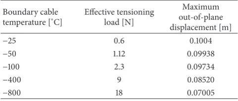
[image:4.600.308.549.202.305.2]

of the maximum out-of-plane deformation and the first three vibration frequencies due to solar radiation pressure, considering several tensioning cases. InTable 3 the results

Table 3: Pretensioning scheme results.

Boundary cable temperature [∘C]

Effective tensioning load [N]

Maximum out-of-plane displacement [m]

−25 0.6 0.1004

−50 1.12 0.09938

−100 2.3 0.09734

−400 9 0.08520

−800 18 0.07005

0.1 0.101 0.102 0.103 0.104 0.105 0.106 0.107 0.108 0.109

0 2 4 6 8 10 12 14 16 18 20

M

axim

um dis

p

lacemen

t (m)

Element number ×103

Figure 3: Mesh sensitivity analysis.

of the structural analysis for the maximum out-of-plane displacements achieved varying the tensioning force at the corners of the membrane are reported. As discussed in Section 3, the tensioning force on the membrane corners was obtained by inducing the shrinkage of the cables. This was achieved by imposing a negative temperature as boundary condition at the nodes of the truss elements. However, it is worth to note that the temperature boundary conditions reported inTable 3are a fictitious thermal load, which is a numerical expedient to generate an effective tension applied to the membrane corners (see(3)).

[image:4.600.308.547.206.526.2]

(5)

X Y

Z X

Y

Z

+8.359e − 09 −8.367e − 03

−3.347e − 02 −4.184e − 02 −5.020e − 02

−6.694e − 02 −7.530e − 02 −8.367e − 02 −9.204e − 02 −1.004e − 01

+1.346e − 07 −5.840e − 03 −1.168e − 02 −1.752e − 02 −2.336e − 02 −2.920e − 02 −3.504e − 02 −4.088e − 02 −4.672e − 02 −5.256e − 02 −5.840e − 02 −6.424e − 02 −7.008e − 02 −1.673e − 02

−2.510e − 02

−5.857e − 02 U

,

U3

U

,

[image:5.600.60.539.74.278.2]

U3

Figure 4: Out-plane displacement for 0.6 N and 18 N tensioning load [m].

Table 4: Vibration frequency.

Tensioning case 0.6 N Tensioning case 18 N Mode number Frequency [Hz] Mode number Frequency [Hz]

1 3.01406𝐸 − 02 1 3.40415𝐸 − 02

2 3.04789𝐸 − 02 2 3.61394𝐸 − 02

3 3.11011𝐸 − 02 3 3.73543𝐸 − 02

4 3.77720𝐸 − 02 4 3.79401𝐸 − 02

displacements obtained with the minimum tensioning force (on the left) and the maximum tensioning force (on the right), in the case of a maximum thrust during a 35-degree manoeuvre. The two displacement distributions are similar, but the maximum displacement value is largely reduced in case of tensioning at 18 N. The load required to tension the sail membrane properly is an important design key factor, because it affects the wrinkles’ formation on the sail membrane [30], and it is limited by structural stability of the booms.

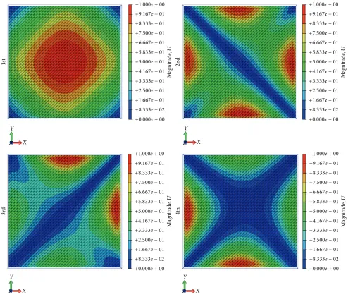
The last part of the FEM analysis investigates the natural vibration modes of the solar-sail membrane for the different pretensioning cases. The results are reported inTable 4, where it can be observed that the vibration modes shift to higher frequencies with the increasing of the pretensioning load. These results can be related to the membrane stress state, which is directly influenced by the intensity of the tensioning load. An increase of such loads corresponds to an increase of the vibration frequency. The total displacements associated with the first four modes of the 0.6 N and 18 N tensioning cases are shown in Figures5and6, respectively. Comparing the images in Figures 5and6, it can be observed that the shapes of the modes encountered in the 0.6 N tensioning

case are different from those of the 18 N tensioning one. This difference may be explained by the loose state of the membrane in case of tension at 0.6 N. Further, the 0.6 N tension load is the lowest value of the tension force to reach the numerical convergence of the solution in the static analysis, but this value may add some uncertainties to the dynamic analysis. In fact, we noted that, in the case of pretensioning at 0.6 N, the first four modes of the solar-sail membrane presented shapes similar to ones reported inFigure 6, which are the typical shape modes of a square membrane.

3.3. Determination of the Structural Offset. The disturbing

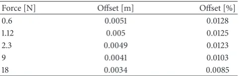
offset was determined using a Matlab script for each ten-sioning case. In this calculation, the model was simplified assuming that the booms could withstand the axial loads due to the sail tensioning and that the wrinkles of the membrane were negligible. This approach allowed us to investigate the maximum tensioning load required to reduce as much as possible the offset. The offset position on the sail plane (̂𝑗, ̂𝑘)is greatly influenced by the SRP modelling. The solar vector is given by two components, one along the negative ̂𝑖direction and one along the negative ̂𝑗direction. Because of the symmetry of the structures, the same conclusion can be obtained considerinĝ𝑘direction instead of ̂𝑗direction. Results of these calculations are reported inTable 5, where it can be noted that an increased load grants an offset reduction due to the increasing of the in-plane membrane stiffness. In particular, the solar-sail configuration proposed in this work has a smaller offset than the one for the classical X-shape configuration reported in literature [26].

[image:5.600.52.292.361.438.2]

(6)

1

st

2

nd

3

rd ₄th

M

agni

tude

,

U

X Y

Z X

Y

Z

X Y

Z X

Y

Z +1.000e + 00 +9.167e − 01 +8.333e − 01 +7.500e − 01 +6.667e − 01 +5.833e − 01 +5.000e − 01 +4.167e − 01 +3.333e − 01 +2.500e − 01 +1.667e − 01

+0.000e + 00

M

agni

tude

,

U

+1.000e + 00 +9.167e − 01 +8.333e − 01 +7.500e − 01 +6.667e − 01 +5.833e − 01 +5.000e − 01 +4.167e − 01 +3.333e − 01 +2.500e − 01 +1.667e − 01

+0.000e + 00

M

agni

tude

,

U

+1.000e + 00 +9.167e − 01 +8.333e − 01 +7.500e − 01 +6.667e − 01 +5.833e − 01 +5.000e − 01 +4.167e − 01 +3.333e − 01 +2.500e − 01 +1.667e − 01

+0.000e + 00

M

agni

tude

,

U

+1.000e + 00 +9.167e − 01 +8.333e − 01 +7.500e − 01 +6.667e − 01 +5.833e − 01 +5.000e − 01 +4.167e − 01 +3.333e − 01 +2.500e − 01 +1.667e − 01

+0.000e + 00

+8.333e − 02 +8.333e − 02

[image:6.600.54.548.74.491.2]

+8.333e − 02 +8.333e − 02

Figure 5: First four vibration modes for 0.6 N loading case.

Table 5: Offset calculation results.

Force [N] Offset [m] Offset [%]

0.6 0.0051 0.0128

1.12 0.005 0.0125

2.3 0.0049 0.0123

9 0.0041 0.0103

18 0.0034 0.0085

dynamics analysis. In particular, the dynamics analysis con-sidered only the worst case offset scenario, which is the minimum applicable tensioning force (0.6 N) and is the 0.0128% of the sail edge size. The new sail concept is stiffer and guarantees a smaller offset than the X-shape one, which is 0.25% of the sail edge size [26].

4. Dynamics Sailcraft Performances

Due to dislocated mass, the proposed sailcraft’s configuration is characterised by moments of inertia greater than the classical one. Therefore the study of the performances for an attitude manoeuvre is essential to understand whether this architecture can be a valid flight configuration. A 35-degree manoeuvre is taken into account to compare these performances with literature data. Note that, due to slow dynamics, classical interplanetary missions require small-amplitude manoeuvres per day [37,38], while a fast manoeu-vre is required only for “nonclassical” interplanetary missions [39, 40]. A body reference frame {𝑂, ̂𝑖, ̂𝑗, ̂𝑘} is considered for modelling sailcraft attitude dynamics, as described in Section 2.

[image:6.600.51.292.565.642.2]

(7)

1

st

2

nd

3

rd ₄th

X Y

Z X

Y

Z

X Y

Z X

Y

Z

M

agni

tude

,

U

+1.000e + 00 +9.167e − 01 +8.333e − 01 +7.500e − 01 +6.667e − 01 +5.833e − 01 +5.000e − 01 +4.167e − 01 +3.333e − 01 +2.500e − 01 +1.667e − 01

+0.000e + 00

M

agni

tude

,

U

+1.000e + 00 +9.167e − 01 +8.333e − 01 +7.500e − 01 +6.667e − 01 +5.833e − 01 +5.000e − 01 +4.167e − 01 +3.333e − 01 +2.500e − 01 +1.667e − 01

+0.000e + 00

M

agni

tude

,

U

+1.000e + 00 +9.167e − 01 +8.333e − 01 +7.500e − 01 +6.667e − 01 +5.833e − 01 +5.000e − 01 +4.167e − 01 +3.333e − 01 +2.500e − 01 +1.667e − 01

+0.000e + 00

M

agni

tude

,

U

+1.000e + 00 +9.167e − 01 +8.333e − 01 +7.500e − 01 +6.667e − 01 +5.833e − 01 +5.000e − 01 +4.167e − 01 +3.333e − 01 +2.500e − 01 +1.667e − 01

+0.000e + 00

+8.333e − 02 +8.333e − 02

[image:7.600.52.554.72.493.2]

+8.333e − 02 +8.333e − 02

Figure 6: First four vibration modes for 18 N loading case.

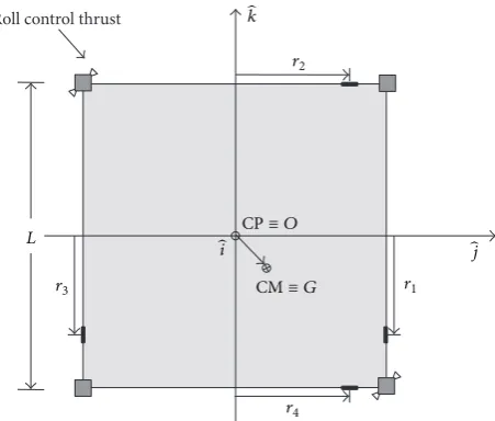
along 𝑘-axis and masses 2 and 4 shift only along 𝑗-axis (Figure 7). The coordinates of the masses are reported in(4), where𝐿is the sail side length and𝑟_𝑖∈ [−𝐿/2, 𝐿/2]

r₁=[[_[

[ 0 𝐿 2 𝑟₁

] ] ] ] ,

r₂=

[ [ [ [ [ 0 𝑟₂ 𝐿 2 ] ] ] ] ] ,

r3= [[

[ 0 −𝐿

2 𝑟₃

] ] ] ,

r4=

[ [ [ [

0 𝑟₄

−𝐿 2 ] ] ] ] .

(4)

The sailcraft attitude dynamics is as follows [41]:

𝑑h0

(8)

L

Roll control thrust ̂k

r1 r2

r3

r4

̂j ̂i

CP≡ O

[image:8.600.59.285.72.264.2]

CM≡ G

Figure 7: Solar-sail configuration scheme.

whereh₀is the angular momentum of the system referred to the origin of body reference𝑂,𝑀is the total sailcraft mass,

a0 is the absolute acceleration of point𝑂, T0 is the torque referred to𝑂, andOGis the position vector of the centre of mass from the reference point𝑂, as shown in

OG= 𝑚_𝑀𝑐

4 ∑

𝑖=1

r_𝑖= 𝑚_𝑀𝑐[[

[ 0 𝑟₂+ 𝑟₄ 𝑟₁+ 𝑟₃ ] ] ]

. (6)

The total angular momentum is given by the angular momen-tum of the bus, booms, and membrane (h₀_,_sail) and the angular momentum of masses for attitude control(h₀_,𝑚). In particularh₀_,_sailis

h₀_,sail= [[

[

𝐽_𝑥 0 0 0 𝐽_𝑦 0 0 0 𝐽_𝑧 ] ] ]

⋅ [[ [

𝜔_𝑥 𝜔_𝑦 𝜔_𝑧 ] ] ]

=J₀_,sail⋅ 𝜔 (7)

andh₀_,𝑚is

h₀_,𝑚=

4 ∑

𝑖=1

J_𝑐,𝑖⋅ 𝜔, (8)

whereJ_𝑐,𝑖is the matrix of inertia due to𝑖th control mass. The

𝜔-term which appears in(7)-(8)is the angular velocity vector of the spacecraft expressed as

𝜔 = 𝜔_𝑥̂𝑖+ 𝜔_𝑦̂𝑗+ 𝜔_𝑧̂𝑘. (9)

The absolute acceleration of the reference point𝑂is expressed by the absolute acceleration of the CM as

a0=a𝐺−𝑑

2_OG 𝑑𝑡2 =

F_𝐺+FSRP

𝑀 −

𝑑2_OG

𝑑𝑡2 , (10)

whereF𝐺is the gravitational force vector and, considering

the simplified solar-sail force model [18], the solar radiation

pressure force vector isFSRP = −2𝜂𝑃𝐴cos2𝛼̂𝑖, where𝑃is the value of SRP at 1 AU(𝑃 = 4.56×10−6N/m2),𝐴is the sail area,𝜂 = 0.85 is the solar-sail efficiency factor, and𝛼is the angle between Sun-line direction and roll axis, as described inSection 2. The torque relative to the origin𝑂is given by the gravitational force and SRP force, as shown in

T0=T𝐺+Toff

≅∑𝑛

𝑖=1

𝑚_𝑖(OG+GP𝑖)

⋅ (−𝜇R𝐺

𝑅3

𝐺

− 𝜇∇ [R𝑖

𝑅3

𝑖

]

𝑅=𝑅𝐺

⋅GP𝑖) + 𝜀 ×FSRP,

(11)

where𝜇is the Sun gravitational constant,GP𝑖is the distance

between CM and the𝑖th point of the sailcraft, and𝜀is the disturbance offset vector. Since ballast masses 1, 3 and 2, 4 are coupled,(5)can be rewritten through the following scalar:

4𝑚_𝑐(𝑟₁ ₁̇𝑟 + 𝑟₂ ₂̇𝑟) 𝜔_𝑥+ [𝐽_𝑥+ 𝑚_𝑐(𝐿2+2𝑟2₁+2𝑟₂2)] ̇𝜔_𝑥

+ [𝐽𝑧− 𝐽𝑦+2𝑚𝑐(𝑟22− 𝑟21)] 𝜔𝑦𝜔𝑧−𝑚

2

𝑐

𝑀[2𝑟2(2 1̈𝑟 +2 ̇𝜔_𝑥𝑟₂+4𝜔_𝑥 ₂̇𝑟 −2𝜔2_𝑦𝑟₁+2𝜔_𝑦𝜔_𝑧𝑟₂) −2𝑟₁(2 ₂̈𝑟

−2 ̇𝜔_𝑥𝑟₁−4𝜔_𝑥 ₁̇𝑟 +2𝜔_𝑦𝜔_𝑧𝑟₁−2𝜔_𝑧2𝑟₂)] = −3𝜇 𝑅3

𝐺

[𝐽_𝑧

− 𝐽_𝑦+2𝑚_𝑐(𝑟₂2− 𝑟₁2)] 𝑎₁₂𝑎₁₃+ 𝜀_𝑦𝐹_𝑧− 𝜀_𝑧𝐹_𝑦,

4𝑚_𝑐𝑟₁ ₁̇𝑟𝜔_𝑦+ [𝐽_𝑦+ 𝑚_𝑐(𝐿 2

2 +2𝑟 2

1)] ̇𝜔𝑦+ [𝐽𝑥− 𝐽𝑧

+ 𝑚_𝑐(𝐿2 2 +2𝑟

2

1)] 𝜔𝑥𝜔𝑧−𝑚

2

𝑐

𝑀 [

2𝐹_SRP 𝑚_𝑐 𝑟1

+2𝑟₁(2 ̇𝜔_𝑦𝑟₁+4𝜔_𝑦 ₁̇𝑟 −2 ̇𝜔_𝑧𝑟₂−4𝜔_𝑧 ₂̇𝑟 +2𝜔_𝑥𝜔_𝑦𝑟₂

+2𝜔_𝑥𝜔_𝑧𝑟₁)] = −3𝜇 𝑅3

𝐺

[𝐽_𝑥− 𝐽_𝑧+ 𝑚_𝑐(𝐿2 2 +2𝑟

2 1)]

⋅ 𝑎₁₁𝑎₁₃+ 𝜀_𝑧𝐹_𝑥− 𝜀_𝑥𝐹_𝑧,

4𝑚_𝑐𝑟₂ ₂̇𝑟𝜔_𝑧+ [𝐽_𝑧+ 𝑚_𝑐(𝐿 2

2 +2𝑟 2

2)] ̇𝜔𝑧+ [𝐽𝑦− 𝐽𝑥

− 𝑚_𝑐(𝐿2 2 +2𝑟

2

2)] 𝜔𝑥𝜔𝑦−𝑚

2

𝑐

𝑀[−

2𝐹_SRP 𝑚_𝑐 𝑟2

−2𝑟₂(2 ̇𝜔_𝑦𝑟₁+4𝜔_𝑦 ₁̇𝑟 −2 ̇𝜔_𝑧𝑟₂−4𝜔_𝑧 ₂̇𝑟 +2𝜔_𝑥𝜔_𝑦𝑟₂

+2𝜔_𝑥𝜔_𝑧𝑟₁)] = 3𝜇 𝑅3

𝐺

[𝐽_𝑦− 𝐽_𝑥− 𝑚_𝑐(𝐿2 2 +2𝑟

2 2)]

⋅ 𝑎₁₁𝑎₁₂+ 𝜀_𝑥𝐹_𝑦− 𝜀_𝑦𝐹_𝑥,

(12)

(9)

expressed in body reference as ̂𝑅_𝐺 = 𝑎₁₁̂𝑖 + 𝑎₁₂̂𝑗 + 𝑎₁₃̂𝑘 and depend on the set of rotations chosen for the attitude representation. Let us call (𝜑, 𝜗, 𝜓), respectively, the roll, pitch, and yaw angles of the spacecraft relative to the orbital reference frame, obtained by a rotational sequence of𝑅₃_(𝜓)− 𝑅2(𝜗)−𝑅1(𝜑)from the orbital to the body reference frame. The

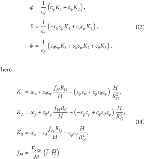
kinematics equations are

̇𝜑 = _𝑐1

𝜗(𝑐𝜓𝐾1+ 𝑠𝜓𝐾2) ,

̇𝜗 = 1

𝑐_𝜗(−𝑐𝜗𝑠𝜓𝐾1+ 𝑐𝜗𝑐𝜓𝐾2) ,

̇𝜓 =_𝑐1

𝜗(𝑠𝜗𝑐𝜓𝐾1+ 𝑠𝜗𝑠𝜓𝐾2+ 𝑐𝜗𝐾3) ,

(13)

where

𝐾₁= 𝜔_𝑥+ 𝑐_𝜗𝑐_𝜓𝑓𝐻_𝐻𝑅𝐺− (𝑠_𝜑𝑠_𝜓+ 𝑐_𝜑𝑠_𝜗𝑐_𝜓)_𝑅𝐻₂

𝐺,

𝐾2= 𝜔𝑦+ 𝑐𝜗𝑠𝜓𝑓𝐻_𝐻𝑅𝐺− (−𝑠𝜑𝑐𝜓+ 𝑐𝜑𝑠𝜗𝑠𝜓)_𝑅𝐻2

𝐺,

𝐾₃= 𝜔_𝑧− 𝑠_𝜗𝑓𝐻𝑅𝐺

𝐻 − 𝑐𝜑𝑐𝜗 𝐻 𝑅2

𝐺

,

𝑓_𝐻= 𝐹SRP

𝑀 (̂𝑖⋅ ̂𝐻)

(14)

is the force per unit mass in the orbital angular momentum direction ( ̂𝐻). In order to achieve the desired manoeu-vre, a combination of feedforward and feedback control, as described in [42, 43], is used. In Sections 4.1 and 4.2 feedforward and feedback methods are briefly presented.

4.1. The Feedforward Controller. Feedforward control is based

on a parameterisation of a desired manoeuvre, expressed as a nth-order polynomial in the generic angle 𝜁. The order of polynomial depends on the boundary conditions and it should not be too big to reduce wandering phenomena. A seventh-order polynomial has been considered in this study as follows:

𝜁 (𝑡) = 𝜁𝑑(𝐴𝜏7+ 𝐵𝜏6+ 𝐶𝜏5+ 𝐷𝜏4+ 𝐸𝜏3+ 𝐹𝜏2+ 𝐺𝜏

+ 𝐻) , (15)

[image:9.600.310.550.86.163.2] [image:9.600.56.296.172.431.2]

where 𝜁_𝑑 is the desired angle of manoeuvre and 𝜏 = 𝑡/𝑇_MAN is the nondimensional time. 𝑇_MAN is the final time after the manoeuvre. In order to find the coefficients (𝐴, 𝐵, 𝐶, 𝐷, 𝐸, 𝐹, 𝐺, 𝐻)in(15), the boundary conditions for 𝜁(𝑡)are listed inTable 6.

Table 6: Feedforward boundary conditions.

𝑛 𝑑𝑛𝜁 (𝑡)

𝑑𝑡𝑛 󵄨󵄨󵄨󵄨󵄨󵄨󵄨󵄨_𝑡=0

𝑑𝑛_{𝜁 (𝑡)} 𝑑𝑡𝑛 󵄨󵄨󵄨󵄨󵄨󵄨󵄨󵄨_𝑡=𝑇

MAN

0 0 𝜁_𝑑

1 0 0

2 0 0

3 0 0

According to the boundary conditions in Table 6, the parameterised manoeuvre angle is expressed by the following seventh-order polynomial:

𝜁 (𝑡) = 𝜁𝑑(−20(_𝑇𝑡 MAN

)7+70( 𝑡 𝑇MAN

)6

−84( 𝑡 𝑇MAN

)5+35( 𝑡 𝑇MAN

)4) .

(16)

In order to design simply the feedforward controller, the following assumptions are made [42]:

(i) Inertia matrix is diagonal and constant, not affected by the position of control masses.

(ii) SRP force is the only force acting on the sailcraft.

(iii) The centre of mass lies on sail plane(̂𝑗, ̂𝑘).

With the hypothesis above, Euler equation is simply given by

J⋅ ̇𝜔 + 𝜔 ×J⋅ 𝜔 =T_𝐶+Toffset, (17)

whereT𝐶is the control torque:

T𝐶= [𝑇𝐶,𝑥, − 𝐹SRP2_𝑀𝑚𝑐𝑧, 𝐹SRP2_𝑀𝑚𝑐𝑦]

𝑇

. (18)

Using(17)-(18)and defining𝛽as the angle between Euler axis and pitch axis, the feedforward control law for masses is given by

𝑦 (𝑡) = 𝑀 2𝑚_𝑐𝜀𝑦−

𝑀𝐽_𝑧 ̈𝜁(𝑡)sin𝛽 2𝐹SRP𝑚𝑐

,

𝑧 (𝑡) = 𝑀 2𝑚_𝑐𝜀𝑧+

𝑀𝐽_𝑦 ̈𝜁(𝑡)cos𝛽 2𝐹SRP𝑚𝑐 .

(19)

To comply with geometrical boundaries, the dynamical scal-ing of the manoeuvre time𝑇_MAN∗ is used [44]:

𝑇MAN∗ = 𝑐 ⋅ 𝑇MAN, (20)

where

𝑐 =max(√sgn(𝑦

∗_{) (𝑦}∗_{− (𝑀/}₂_𝑚

𝑐) 𝜀𝑦)

𝑦_max− (𝑀/2𝑚_𝑐) 𝜀_𝑦sgn(𝑦∗),

√sgn(𝑧∗) (𝑧∗− (𝑀/2𝑚𝑐) 𝜀𝑧)

𝑧_max− (𝑀/2𝑚_𝑐) 𝜀_𝑧sgn(𝑧∗)) .

(10)

CM CP 1 2

3

4 To the Sun

Yaw manoeuvre

̂k

̂j

̂i

(a)

CM

CP 1 2

3

4 To the Sun

Pitch manoeuvre

̂k

̂j

̂i

[image:10.600.105.499.72.285.2]

(b)

Figure 8: Schematisation of yaw (a) and pitch (b) manoeuvre.

𝑦∗and𝑧∗are the maximum shift of control masses required along the𝑗-axis and𝑘-axis, respectively.

4.2. The Feedback Controller. The pitch/yaw feedback control

is based on the error between the desired manoeuvre and the one carried out by the sailcraft. The feedback control logic is in Proportional-Integral-Derivative (PID) form as below [26]:

𝑢 = − 𝐾_𝐷 ̇𝑒− 𝐾𝑃𝑒 − 𝐾𝐼∫ 𝑒d𝑡, (22)

where 𝑒 is the error between desired angle and real one and 𝐾_𝐷, 𝐾_𝑃, and 𝐾_𝐼 are the derivative, proportional, and integral gain, respectively. This control can be decoupled in each axis and gains can be determined as Single-Input-Single-Output (SISO) problem. Of course, whenever tuning a gain, the system response changes and the best gains are iteratively set.

A rate limiter and a saturation limit are added to sim-ple PID controller, because of mechanical and geometrical boundaries. These boundaries are

𝑢_max= 𝐿 2,

̇𝑢max= 𝑢_TCmax,

(23)

where TC = 560 s is the actuator time constant taken into account, according to the value in [26]. The roll feedback control is performed with on-off controllers that work when the tolerance on roll angle is exceeded. The controller chosen is a set of 4 PPTs positioned coupled on 2 opposite satellites and the average thrust of each PPT chosen is 150𝜇N [45]. For this study, a required roll angle of 0 degrees with a tolerance of±0.1 degrees is set, so that the thrusters switch on when the roll angle exceeds this value.

4.3. Numerical Results. Numerical simulations are carried

[image:10.600.318.548.461.568.2]

out in order to verify the performances of the proposed con-figuration. As reported in previous sections, a feedforward controller was used to generate the desired manoeuvre over time and a feedback controller with PID logic was set to control the nonmodelled trends in feedforward controller. The characteristics of the sailcraft are those reported in Table 1, while velocities and accelerations of masses in (12) are considered null [26,28]. The attitude is represented by the rotational matrix which transforms body into orbital reference frame:

[ [ [ [

̂𝑅𝐺

̂𝜃 ̂ 𝐻 ] ] ] ]

=[[_[ [

−𝑐_𝜗𝑐_𝜓 −𝑐_𝜗𝑠_𝜓 𝑠_𝜗

𝑐_𝜑𝑠_𝜓− 𝑠_𝜑𝑠_𝜗𝑐_𝜓 −𝑐_𝜑𝑐_𝜓− 𝑠_𝜑𝑠_𝜗𝑠_𝜓 −𝑠_𝜑𝑐_𝜗 𝑠_𝜑𝑠_𝜓+ 𝑐_𝜑𝑠_𝜗𝑐_𝜓 −𝑠_𝜑𝑐_𝜓+ 𝑐_𝜑𝑠_𝜗𝑠_𝜓 𝑐_𝜑𝑐_𝜗

] ] ] ]

[ [ [ [ ̂𝑖 ̂𝑗 ̂𝑘 ] ] ] ] .

(24)

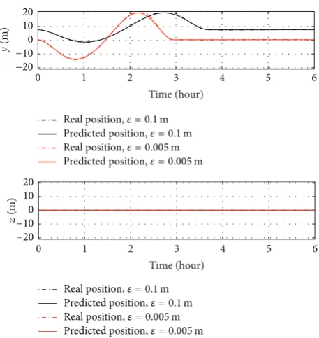
In order to evaluate the performances of the proposed configuration, a 35-degree manoeuvre in a circular planar Earth-like orbit is considered. InFigure 8(a)a 35-degree yaw manoeuvre with disturbance offset on𝑗-axis is schematically represented; inFigure 8(b)a 35-degree pitch manoeuvre with disturbance offset on𝑗-axis is schematically represented.

First, a 35-degree yaw manoeuvre without offset (CP ≡ 𝑂) is performed. Time histories of Euler angles and control masses over time are shown in Figures9and10.

(11)

0 1 2 3 4 5 6 Time (hour)

0 1 2 3 4 5 6

Time (hour)

0 1 2 3 4 5 6

Time (hour) −0.2

−0.5

Real𝜃 Predicted𝜃

𝜃

(deg.)

Real𝜓 Predicted𝜓

𝜓

(deg.)

0 0.2

0 0.5

0 20 40

Real_𝜑

Predicted_𝜑

𝜑

[image:11.600.56.289.69.326.2]

(deg.)

Figure 9: Euler angles over time for a 35-degree yaw manoeuvre without offset.

0 1 2 3 4 5 6

0 10 20

Time (hour)

0 10 20

0 1 2 3 4 5 6

Time (hour)

Real position Predicted position Real position Predicted position −20

−10

−20

−10

y

(m)

z

[image:11.600.315.544.72.320.2]

(m)

Figure 10: Positions of sliding masses over time for a 35-degree yaw manoeuvre without offset.

the feedforward controller. However, no evident differences between real angles and predicted ones are visible byFigure 9. The analysis with offset takes into account only the maximum offset calculated inSection 3.3, in order to have a worst-case analysis. Figures 11 and 12 show a 35-degree yaw manoeuvre with 0.005 m offset (red curve) and with the literature one of 0.1 m (black curve).

Similar to the case without offset, roll and pitch angles do not change from initial conditions and real and predicted angles overlap. The manoeuvre with the offset presented in

0 0.2

0 0.5

0 20 40

−0.2

−0.5

𝜑

(deg.)

𝜃

(deg.)

𝜓

(deg.)

0 1 2 3 4 5 6

Time (hour)

Real_𝜑,_{𝜀 = 0.1}m

Predicted_𝜑,_{𝜀 = 0.1}m

Real_𝜑,_{𝜀 = 0.005}m

Predicted_𝜑,_{𝜀 = 0.005}m

0 1 2 3 4 5 6

Time (hour)

Real_𝜃,_{𝜀 = 0.1}m

Predicted_𝜃,_{𝜀 = 0.1}m

0 1 2 3 4 5 6

Time (hour)

Real𝜓,𝜀 = 0.1m

Predicted𝜓,𝜀 = 0.1m

Real_𝜃,_{𝜀 = 0.005}m

Predicted_𝜃,_{𝜀 = 0.005}m

Real𝜓,𝜀 = 0.005m

[image:11.600.55.287.376.585.2]

Predicted𝜓,𝜀 = 0.005m

Figure 11: Euler angles over time for a 35-degree yaw manoeuvre with disturbance offset on𝑗-axis.

0 10 20

0 1 2 3 4 5 6

Time (hour)

0 1 2 3 4 5 6

Time (hour)

−20 −10

y

(m)

z

(m)

Real position,𝜀 = 0.1m

Predicted position,𝜀 = 0.1m Real position,𝜀 = 0.005m Predicted position,𝜀 = 0.005m

Real position,𝜀 = 0.1m

Predicted position,𝜀 = 0.1m Real position,𝜀 = 0.005m Predicted position,𝜀 = 0.005m

Figure 12: Positions of sliding masses over time for a 35-degree yaw manoeuvre with disturbance offset on𝑗-axis.

[image:11.600.315.544.381.623.2]

(12)

0 0.1 0.2

0 20 40

0 0.5

0 1 2 3 4 5 6

Time (hour)

0 1 2 3 4 5 6

Time (hour)

0 1 2 3 4 5 6

Time (hour) −0.2

−0.1

−0.5

Real𝜃 Predicted𝜃

𝜃

(deg.)

Real𝜓 Predicted𝜓

𝜓

(deg.)

Real_𝜑

Predicted_𝜑

𝜑

[image:12.600.55.290.68.328.2]

(deg.)

Figure 13: Euler angles over time for a 35-degree pitch manoeuvre with 0.005 m offset on𝑗-axis.

steady-state position of each sliding mass can be simply obtained by(19), as shown in

𝑦ss(𝑡) =

𝑀 2𝑚_𝑐𝜀𝑦,

𝑧ss(𝑡) =

𝑀 2𝑚_𝑐𝜀𝑧.

(25)

As shown inFigure 12and in(25), the steady-state position of the sliding masses on 𝑗-axis is 𝑦ss = 7.65 m with the

literature offset of 0.1 m; on the other hand, for an offset value of 0.005 m, the steady-state position of the control masses on 𝑗-axis is only𝑦ss=0.38 m.

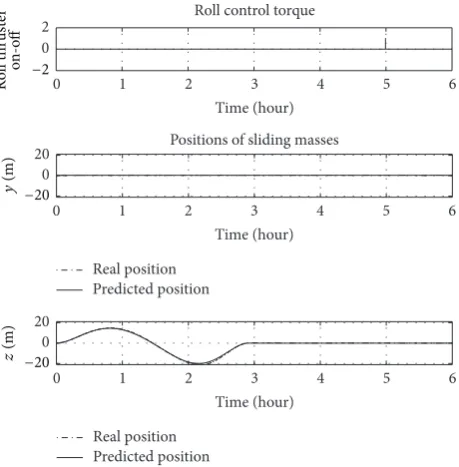
As shown from Figures9to12, no roll control is necessary during a 35-degree yaw manoeuvre with offset on 𝑗-axis, because the roll angle is null during the entire manoeuvre. Figures13and14show that for a 35-degree pitch manoeuvre with a disturbance offset on the same axis a roll control is necessary.

Figure 13shows that in a pitch manoeuvre the roll angle decreases slowly, so that only after about 5 hours does the roll controller act, due to the threshold set to 0.1 degrees. For missions that require different attitude accuracy, this threshold can be set to different values. Excluding the time history of roll angle, the manoeuvre is completed as well as in the previous examples.

Comparing these manoeuvres with those in literature, a 35-degree yaw manoeuvre presented in [26] and a 30-degree pitch manoeuvre presented in [28] are both completed in about 2 hours. The manoeuvre presented in [42] for a perfectly reflecting solar sail is much faster than the one

0 2

Roll control torque

0

20 Positions of sliding masses

0 20

Ro

ll t

h

ru

st

er

o

n-o

ff

0 1 2 3 4 5 6

Time (hour)

Real position Predicted position

0 1 2 3 4 5 6

Time (hour)

−20 −2

0 1 2 3 4 5 6

Time (hour)

Real position Predicted position −20

y

(m)

z

[image:12.600.316.546.73.307.2]

(m)

Figure 14: Attitude controls over time for a 35-degree pitch manoeuvre with 0.005 m offset on𝑗-axis.

presented here, due to the higher moments of inertia of the proposed architecture. As mentioned above, high moments of inertia are a disadvantage for an attitude manoeuvre and one of the aims of this study is to ensure the manoeuvrability of this configuration. However, in interplanetary trajectories a fast manoeuvre is not always required and the configuration presented has performances compatible with the most chal-lenging interplanetary missions.

5. Conclusions

(13)

flight. In addition, it is worth noting that in the classical X-configuration the effective area for a 40 m side sail is 1200 m2 instead of 1600 m2, due to the membrane deformation and the fact that around the booms there is no membrane. On the contrary, in the proposed configuration the disposition of the booms along the perimeter and the deformation of the membrane allow one to consider a major effective area, closer to nominal value of 1600 m2. Starting from these results, numerical simulations of the attitude manoeuvres demonstrated that the proposed architecture gives good per-formances, despite the large moments of inertia. It was shown that a 35-degree manoeuvre can be completed in less than 3 hours, according to the usual requirements for interplanetary missions. The new solar-sail concept is proposed for an interplanetary mission, but advantages of this configuration are useful also for planetary missions. In general, the principal constraint that must be taken into account is the velocity of change attitude manoeuvres. In fact, for a planetary mission, around the nodal line a fast change on the sail attitude can be necessary; this event can be critical for this configuration and the performances must be evaluated case by case. On the contrary the higher moment of inertia can be favourable for missions where the sail attitude must remain constant (but this is valid also for the interplanetary case). In all cases studied, the disturbing torque, caused by structural offset, determines the steady-state positions of the sliding masses. As a consequence, the small offset value of this sail configuration guarantees a great increase in manoeuvrability.

Conflict of Interests

The authors declare that there is no conflict of interests regarding the publication of this paper.

References

[1] M. MacDonald and C. R. McInnes, “Solar sail science mission applications and advancement,”Advances in Space Research, vol. 48, no. 11, pp. 1702–1716, 2011.

[2] C. Circi, “Mars and mercury missions using solar sails and solar electric propulsion,”Journal of Guidance, Control, and Dynam-ics, vol. 27, no. 3, pp. 496–498, 2004.

[3] B. Dachwald and W. Seboldt, “Multiple near-Earth asteroid rendezvous and sample return using first generation solar sailcraft,”Acta Astronautica, vol. 57, no. 11, pp. 864–875, 2005. [4] G. Mengali, A. A. Quarta, C. Circi, and B. Dachwald, “Refined

solar sail force model with mission application,” Journal of Guidance, Control, and Dynamics, vol. 30, no. 2, pp. 512–520, 2007.

[5] G. Aliasi, G. Mengali, and A. A. Quarta, “Passive control feasibility of collinear equilibrium points with solar balloons,” Journal of Guidance, Control, and Dynamics, vol. 35, no. 5, pp. 1657–1661, 2012.

[6] M. Ceriotti and C. R. McInnes, “Systems design of a hybrid sail pole-sitter,”Advances in Space Research, vol. 48, no. 11, pp. 1754– 1762, 2011.

[7] M. Ceriotti and C. R. McInnes, “Generation of optimal trajecto-ries for Earth hybrid pole sitters,”Journal of Guidance, Control, and Dynamics, vol. 34, no. 3, pp. 847–859, 2011.

[8] J. Heiligers, M. Ceriotti, C. R. McInnes, and J. D. Biggs, “Dis-placed geostationary orbit design using hybrid sail propulsion,” Journal of Guidance, Control, and Dynamics, vol. 34, no. 6, pp. 1852–1866, 2011.

[9] J. Simo and C. R. McInnes, “Solar sail orbits at the Earth-Moon libration points,” Communications in Nonlinear Science and Numerical Simulation, vol. 14, no. 12, pp. 4191–4196, 2009. [10] J. Simo and C. R. McInnes, “Asymptotic analysis of displaced

lunar orbits,”Journal of Guidance, Control, and Dynamics, vol. 32, no. 5, pp. 1666–1670, 2009.

[11] P. Anderson and M. Macdonald, “Extension of highly elliptical earth orbits using continuous low-thrust propulsion,”Journal of Guidance, Control, and Dynamics, vol. 36, no. 1, pp. 282–292, 2013.

[12] P. Anderson and M. Macdonald, “Static, highly elliptical orbits using hybrid low-thrust propulsion,”Journal of Guidance, Con-trol, and Dynamics, vol. 36, no. 3, pp. 870–880, 2013.

[13] G. Mengali and A. A. Quarta, “Solar sail trajectories with piecewise-constant steering laws,”Aerospace Science and Tech-nology, vol. 13, no. 8, pp. 431–441, 2009.

[14] B. Dachwald, “Optimization of very-low-thrust trajectories using evolutionary neurocontrol,”Acta Astronautica, vol. 57, no. 2–8, pp. 175–185, 2005.

[15] T. Ingrassia, V. Faccin, A. Bolle, C. Circi, and S. Sgubini, “Solar sail elastic displacement effects on interplanetary trajectories,” Acta Astronautica, vol. 82, no. 2, pp. 263–272, 2013.

[16] C. Circi, “Three-axis attitude control using combined gravity-gradient and solar pressure,”Proceedings of the Institution of Mechanical Engineers, Part G: Journal of Aerospace Engineering, vol. 221, no. 1, pp. 85–90, 2007.

[17] G. Mengali and A. A. Quarta, “Near-optimal solar-sail orbit-raising from low earth orbit,”Journal of Spacecraft and Rockets, vol. 42, no. 5, pp. 954–958, 2005.

[18] C. R. McInnes,Solar Sailing: Technology, Dynamics and Mission Applications, Springer Praxis Publishing, Chichester, UK, 2004. [19] L. Johnson, R. Young, E. Montgomery, and D. Alhorn, “Status of solar sail technology within NASA,”Advances in Space Research, vol. 48, no. 11, pp. 1687–1694, 2011.

[20] L. Johnson, M. Whorton, A. Heaton, R. Pinson, G. Laue, and C. Adams, “NanoSail-D: a solar sail demonstration mission,”Acta Astronautica, vol. 68, no. 5-6, pp. 571–575, 2011.

[21] V. Lappas, N. Adeli, L. Visagie et al., “CubeSail: a low cost Cube-Sat based solar sail demonstration mission,”Advances in Space Research, vol. 48, no. 11, pp. 1890–1901, 2011.

[22] U. Geppert, B. Biering, F. Lura, J. Block, M. Straubel, and R. Reinhard, “The 3-step DLR–ESA gossamer road to solar sailing,”Advances in Space Research, vol. 48, no. 11, pp. 1695– 1701, 2011.

[23] Y. Tsuda, O. Mori, R. Funase et al., “Achievement of IKAROS— Japanese deep space solar sail demonstration mission,” Acta Astronautica, vol. 82, no. 2, pp. 183–188, 2013.

[24] C. Sickinger, L. Herbeck, and E. Breitbach, “Structural engineer-ing on deployable CFRP booms for a solar propelled sailcraft,” Acta Astronautica, vol. 58, no. 4, pp. 185–196, 2006.

[25] A. Stabile and S. Laurenzi, “Coiling dynamic analysis of thin-walled composite deployable boom,”Composite Structures, vol. 113, no. 1, pp. 429–436, 2014.

(14)

[27] B. Wie, D. Murphy, M. Paluszek, and S. Thomas, “Robust atti-tude control systems design for solar sail, part 1: propellantless primary ACS,” inProceedings of the AIAA Guidance, Navigation, and Control Conference and Exhibit, Providence, RI, USA, 2004. [28] S. N. Adeli, V. J. Lappas, and B. Wie, “A scalable bus-based attitude control system for Solar Sails,” Advances in Space Research, vol. 48, no. 11, pp. 1836–1847, 2011.

[29] B. Wie, “Solar sail attitude control and dynamics, part 1,”Journal of Guidance, Control, and Dynamics, vol. 27, no. 4, pp. 526–535, 2004.

[30] W. Wong and S. Pellegrino, “Wrinkled membranes III: numer-ical simulations,”Journal of Mechanics of Materials and Struc-tures, vol. 1, no. 1, pp. 63–95, 2006.

[31] D. W. Sleight and D. M. Muheim, “Parametric studies of square solar sails using finite element analysis,” inProceedings of the 45th AIAA/ASME/ASCE/AHS/ASC Structures, Structural Dynamics & Materials Conference, AIAA-2004-1509, Palm Springs, Calif, USA, April 2004.

[32] S. C. Gajbhiye, S. H. Upadhayay, and S. P. Harsha, “Free vibration analysis of flat thin membrane,”International Journal of Engineering Science and Technology, vol. 4, no. 8, pp. 3942– 3948, 2012.

[33] I. Abaqus,Abaqus Analysis User’s Manual, 2010.

[34] J. M. Fernandez, V. J. Lappas, and A. J. Daton-Lovett, “Com-pletely stripped solar sail concept using bi-stable reeled com-posite booms,”Acta Astronautica, vol. 69, no. 1-2, pp. 78–85, 2011.

[35] D. W. Sleight, T. Mann, D. Lichodziejewski, and B. Derbes, “Structural analysis and test comparison of a 20-meter inflation-deployed solar sail,” inProceedings of the 47th AIAA/ASME/ ASCE/AHS/ASC Structures, Structural Dynamics and Materials Conference, pp. 1408–1423, May 2006.

[36] S. Laurenzi, D. Barbera, and M. Marchetti, “Buckling design of boom structures by FEM analysis,” inProceedings of the 63rd International Astronautical Congress (IAC ’12), pp. 6367–6371, Naples, Italy, October 2012.

[37] A. Bolle and C. Circi, “Solar sail attitude control through in-plane moving masses,”Proceedings of the Institution of Mechan-ical Engineers, Part G: Journal of Aerospace Engineering, vol. 222, no. 1, pp. 81–94, 2008.

[38] G. Colasurdo and L. Casalino, “Optimal control law for interplanetary trajectories with nonideal solar sail,”Journal of Spacecraft and Rockets, vol. 40, no. 2, pp. 260–265, 2003. [39] G. Mengali, A. A. Quarta, D. Romagnoli, and C. Circi,

“H2-reversal trajectory: a new mission application for high-performance solar sails,”Advances in Space Research, vol. 48, no. 11, pp. 1763–1777, 2011.

[40] G. Vulpetti, “3D high-speed escape heliocentric trajectories by all-metallic-sail low-mass sailcraft,”Acta Astronautica, vol. 39, no. 1–4, pp. 161–170, 1996.

[41] B. Wie, “Solar sail attitude control and dynamics, part 2,”Journal of Guidance, Control, and Dynamics, vol. 27, no. 4, pp. 536–544, 2004.

[42] D. Romagnoli and T. Oehlschl¨agel, “High performance two degrees of freedom attitude control for solar sails,”Advances in Space Research, vol. 48, no. 11, pp. 1869–1879, 2011.

[43] C. Scholz, D. Romagnoli, B. Dachwald, and S. Theil, “Perfor-mance analysis of an attitude control system for solar sails using sliding masses,”Advances in Space Research, vol. 48, no. 11, pp. 1822–1835, 2011.

[44] B. Siciliano, L. Sciavicco, L. Villani, and G. Oriolo,Robotics— Modelling, Planning and Control, Advanced Textbooks in Con-trol and Signal Processing, Springer, London, UK, 2009. [45] B. Wie, D. Murphy, M. Paluszek, and S. Thomas, “Robust

(15)