Do-Validation for Kernel Density Estimation

      

City, University of London Institutional Repository

Citation:

Mammen, E., Martinez-Miranda, M. D., Nielsen, J. P. and Sperlich, S. (2011). Do-Validation for Kernel Density Estimation. Journal of the American Statistical Association, 106(494), pp. 651-660. doi: 10.1198/jasa.2011.tm08687

This is the accepted version of the paper.

This version of the publication may differ from the final published

version.

Permanent repository link:

http://openaccess.city.ac.uk/4633/

Link to published version:

http://dx.doi.org/10.1198/jasa.2011.tm08687

Copyright and reuse: City Research Online aims to make research

outputs of City, University of London available to a wider audience.

Copyright and Moral Rights remain with the author(s) and/or copyright

holders. URLs from City Research Online may be freely distributed and

linked to.

City Research Online: http://openaccess.city.ac.uk/ [email protected]

Do-validation for Kernel Density Estimation

Enno Mammen

Universit¨

at Mannheim, Abteilung Volkswirtschaftslehre

L7, 3-5, 68131-Mannheim

Mar´ıa Dolores Mart´ınez Miranda

Universidad de Granada, Departamento de Estad´ıstica e I.O.

Campus Fuentenueva, E - 18071 Granada

Jens Perch Nielsen

Cass Business School, City University

106 Bunhill Row, UK - London EC1Y 8TZ

Stefan Sperlich

Universit´

e de Gen`

eve, D´

epartement des sciences ´

economiques

Bd du Pont d’Arve 40, CH - 1211 Gen`

eve 4

Abstract

Bandwidth selection in kernel density estimation is one of the fundamental

model selection problems of mathematical statistics. The study of this problem

took major steps forward with the papers of Hall and Marron (1987) and Hall

and Johnstone (1992). Since then focus seems to have been on various versions

of implementing the so called plug-in method aimed at estimating the minimum

mean integrated squared error (MISE). The most successful of these efforts

still seems to be the plug-in method of Sheather and Jones (1991) or Park and

Marron (1990) that we also use as a benchmark in this paper. In this paper we

derive a new theorem deriving the asymptotic theory for linear combinations of

bandwidths obtained from different selectors as e.g. direct and indirect

cross-validation and plug-in, where we take advantage of recent advances in the study

of indirect cross-validation; see Hart and Yi (1998), Hart and Lee (2005) and

Savchuk, Hart and Sheather (2010a,b). We conclude that the slow convergence

of data-driven bandwidths implies that once asymptotic theory is close to that

of plug-in then it is the practical implementation that counts. This insight led

us to a bandwidth selector search with the symmetrized version of onesided

cross-validation as a clear winner. 1

Keywords: bandwidth choice, cross-validation, plug-in, nonparametric

esti-mation.

1_{We acknowledge very helpful comments from two anonymous referees and the editors. This}

research was financially supported by knowledge company Festina Lente, the Spanish Ministerio de

Educacion y Ciencia, projects MTM2008-03010/MTM, and the Deutsche Forschungsgemeinschaft

1

Introduction

Indirect cross-validation is another class of bandwidth selectors. These selectors make use of so-called selection kernels. A bandwidth is chosen for the selection-kernel es-timator by cross-validation and this bandwidth is then rescaled by an appropriate factor to be suitable for the kernel estimator at hand, see Savchuk, Hart and Sheather (2010a). It has been argued that cross-validation is in particular performing well in harder estimation problems. Indirect Cross-validation makes use of this relation by choosing selection kernels for which bandwidth choice is a more difficult estimation problem, see e.g. Section 4 in Hart and Lee (2005) for this point. Appropriate se-lection kernels robustify the bandwidth choice against discretization effects and data rounding. For a detailed discussion, see Savchuk, Hart and Sheather (2010b). One version of the general principle of indirect cross-validation is onesided cross-validation. Onesided cross-validation was originally proposed by Hart and Yi (1998) for local lin-ear regression. In Hart and Lee (2005) it was shown that in contrast to classical cross validation this approach is robust against spurious and nonspurious serial correlation. Onesided cross-validation was extended to our density case by Mart´ınez-Miranda, Nielsen and Sperlich (2009).

simple combination is appealing because of the well known practical experience of plug-in bandwidths to oversmooth, while the almost unbiased cross-validation band-width sometimes have very bad performance because of undersmoothing. Therefore, intuition says that a simple average should improve both, which indeed turns out to be the case. The asymptotic performance of this simple average is much better than for ordinary cross-validation and only slightly worse than for the plug-in method. In practice it outperforms both. This insight led to a search for good finite sample per-formance of combinations of bandwidths with an asymptotic perper-formance close to the plug-in method. The overall winner of this search was a simple combination of the right-sided and the left-sided versions of onesided cross-validation. We call this new bandwidth selector “do-validation” (double onesided cross-validation). The conclu-sion of this paper therefore suggests the do-validation bandwidth as an asymptotically well performing bandwidth selector with excellent finite sample properties.

The paper is organized as follows. In Section 2 we define a new class of combined cross-validation bandwidth selectors. In Section 3 theoretical properties of linear combinations of cross-validated bandwidths and a plug-in bandwidth are derived. In Sections 4 and 5 we consider six bandwidth selectors: the standard cross-validation

two terms. All bandwidths have the same asymptotic first component. The second component varies with the different methods. While it is quite large for the cross-validation method, it is less than one third of this value for all other methods. The exact asymptotic values become less important than the practical performance of the implementation at hand. This is one conclusion of Section 5 where we present results of a finite sample study where do-validation h_DO comes out as the best of the con-sidered methods. Another conclusion is that combinations of certain bandwidths can improve a lot in ISE compared to their individual performance.

2

A general class of data-driven bandwidth

esti-mators

In this paper we consider a class of bandwidth selectors h that are constructed as weighted averages of cross-validation bandwidthsh_j. The aim is to get a bandwidth with a small Integrated Squared Error (ISE) for the kernel density estimator

f_h,K(x) = 1

nh n

i=1

K

X_i−x h

.

The bandwidthsh_jare based on the inspection of kernel density estimatorsf_h,Lj(x),1≤

j ≤ J, for kernels L_j that fulfill L_j(0) = 0. For 1≤j ≤J we define h_j by the cross-validation method

h_j = arg min

h

f_h,Lj(x)2dx−2n−1 n

i=1

f_h,Lj(X_i). (1) Note that because of L_j(0) = 0 we do not need to use a leave-one-out version off_h,Lj

with J_j=1w_j = 1, a new bandwidth selector h is defined by

h =

J

j=1

w_j

R(K)

μ2₂(K)

μ2₂(L_j)

R(L_j)

1/5

h_j (2)

where R(g) = g2(x)dx, μ_l(g) = xlg(x)dx for functions g and integers l ≥ 0. The bandwidth h_j is a selector for the kernel L_j. After multiplying with the fac-tor (R(K)μ2₂(L_j))1/5(μ2₂(K) R(L_j))−1/5 it becomes a selector for the kernel K. This follows from classical smoothing theory and has been used at many places in the discussion of bandwidth selectors.

Our class of bandwidth selectors contains the classical cross-validation bandwidth selector as one example with J = 1 and L₁(u) = K(u)1(u = 0). If one uses a leave-one-out version of (1), one would replacef_h,Lj(X_i) by n(n−1)−1f_h,Lj(X_i) in the second term on the right hand side of (1). This change is asymptotically negligible and does not lead to obvious changes in the finite sample performance. Furthermore, there is a difference if two observations have the same value. Under our assumptions this happens only with zero probability. Thus, our discussion carries over without changes to leave-one-out versions of our proposal.

as kernel density estimator f_h,M∗ with ”equivalent kernel” M∗ given by M∗(u) = μ2(M)−μ1(M)u

μ₀(M)μ₂(M)−μ2₁(M)M(u). (3) In onesided cross-validation the basic kernelM(u) is chosen as 2K(u)1_(−∞,0)(leftsided cross-validation) and 2K(u)1_(0,∞) (rightsided cross-validation). This results in the following equivalent kernels

K_L(u) = μ2(K) +uμ

∗

1(K)

μ₂(K)−(μ∗₁(K))22K(u)1(−∞,0), (4)

K_R(u) = μ2(K)−uμ

∗

1(K)

μ₂(K)−(μ∗₁(K))22K(u)1(0,∞), (5) with μ∗₁(K) =₀∞uK(u)du. Here we have assumed that the kernel K is symmetric. The left-OSCV criterion (OSCV_L) is defined by

OSCV_L(h) =

f_h,K2 _L(x)dx−2n−1 n

i=1

f_h,KL(X_i), (6) with h_L as its minimizer; and the left-OSCV bandwidth is calculated from h_L by

h_L,OSCV= Ch_L,

where

C =

R(K)

μ2₂(K)

μ2₂(K_L)

R(K_L)

_1/5

, (7)

see Mart´ınez-Miranda, Nielsen and Sperlich (2009).

In exactly the same way we define the right-OSCV criterion, OSCV_R, except that

f_h,KL in (6) is replaced by f_h,KR. The right-OSCV bandwidth is calculated by

inferior rate of convergence of the onesided local constant kernel density estimator. This was the reason why Mart´ınez-Miranda, Nielsen and Sperlich (2009) suggested the use of local linear density estimation.

The do-validation selectorh_DO is given by

h_DO = 1

2(hL,OSCV +hR,OSCV).

Left-onesided cross-validation and right-onesided cross-validation are not identical in the local linear case because of differences in the boundary. However, asymptotically they are equivalent. As we will see in our simulations do-validation delivers a good stable compromise. It has the same asymptotic theory as each of the two onesided alternatives and a better overall finite sample performance.

3

Asymptotic theory

In this section we state an asymptotic result on the difference between a combined bandwidth selector h, defined in (2), with the MISE-optimal bandwidth h_MISE and the ISE-optimal bandwidth h_ISE,

h_MISE = arg min

h E

f_h,K(x)−f(x)

₂ dx

,

h_ISE = arg min

h

f_h,K(x)−f(x)

2

dx

.

Under our assumptions, see below, it holds that h_MISE =

R(K)

μ2₂(K)R(f)

1/5

n−1/5+

We are also interested in h∗, with h∗ being a combination with an asymptotical MISE-optimal bandwidth h_MISE defined by

h∗ =

J

j=2

w_j

R(K)

μ2₂(K)

μ2₂(L_j)

R(L_j)

1/5

_{hj+w1hMISE, (8)}

whereJ_j=1w_j = 1 and whereh_MISE is a bandwidth selector withh_MISE =h_MISE+

o_P(n−3/10). In the simulations we will choose h_MISE = h_{P I} where h_{P I} is refers to a plug-in selector along Sheather and Jones (1991) and Park and Marron (1990), respectively.

We now state a theorem about the asymptotic distribution of h−h_MISE, h−h_ISE

and h∗−h_ISE. For this result we need the following assumptions:

(A1) K and L_j (j = 1, . . . , J) are compactly supported. The kernels are continuous onIR− {0}and have one-sided derivatives that are H¨older continuous onIRi.e. there exist constants c, δ > 0 such that |g(x)−g(y)| ≤ c|x−y|δ for x, y < 0 or x, y > 0 with g equal to K or L_j (j = 1, . . . , J). The left- and right-sided derivatives differ at most on a finite set. For j = 1, . . . , J, L_j(0) = 0,

uL_j(u)du= 0 and uK(u)du= 0.

(A2) The density f is bounded and twice differentiable. The derivatives f and f

are bounded and integrable. The second derivative is H¨older continuous with exponent δ > 1₂.

Theorem 1. _{Combination of bandwidths.} Under A1, A2 the bandwidth selector

h in (2) satisfies

n3/10(h−h_ISE) →N(0, σ₁2) in distribution, (9)

n3/10(h−h_MISE) →N(0, σ₂2) in distribution, (10)

where

σ_k2 = 4 25R(K)

−2/5_μ−6/5

2 (K)R(f)−8/5V(f)δk+ 1

50R(K)

−7/5_μ−6/5 2 (K)

×R(f)−3/5R(f) δ_kH(u)−

J

j=1

w_j

R(K)

R(L_j)

H_j(u)

2

du,

(11)

with

V(f) =

f2(x)f(x)dx−

f(x)f(x)dx ₂

,

H(u) = 2

K(u+v)K(v)dv+ 2

K(−u+v)K(v)dv

+2

K(u+v)vK(v)dv+ 2

K(−u+v)vK(v)dv,

H_j(d_ju) = 2

L_j(u+v)L_j(v)dv+ 2

L_j(−u+v)L_j(v)dv

+2

L_j(u+v)vL_j(v)dv+ 2

L_j(−u+v)vL_j(v)dv

−2L_j(u) +uL_j(u) +L_j(−u)−uL_j(−u),

d_j =

R(K)

R(L_j)

μ2₂(L_j)

μ2₂(K)

_−1/5

, δ_k =

⎧ ⎪ ⎪ ⎨ ⎪ ⎪ ⎩

1 for k = 1,

0 for k = 2.

satisfies

n3/10(h∗−h_ISE) →N(0, σ₁2) in distribution, (12)

with σ₁2 as in (11) but with H₁ = 0.

For the special choiceJ = 1, w₁ = 1, the asymptotic expansions in (9), (10) and (12) reduce to the classical results in Hall and Marron (1987), see their Theorem 2.1 and discussions in Section 2.3. Then, equation (12) implies an expansion for the difference between the ISE optimal bandwidth h_ISE and the MISE optimal bandwidth h_MISE

and equations (9) and (10) compare the classical cross-validation bandwidth selector with these two target bandwidths.

Under additional smoothness assumptions onf, Hall and Johnstone (1992) discussed efficient estimation of the ISE-optimal bandwidthh_ISE. They showed that estimation ofh_ISEis asymptotically equivalent to the estimation ofR(f) = f(x)2dx. Using an efficient estimator ofR(f), one gets an estimatorhof h_ISE such thatn3/10(h−h_ISE) has asymptotic variance ₂₅4R(K)−2/5μ₂−6/5(K)R(f)−8/5V(f). Thus, in our class of bandwidth selectors a bandwidth would achieve the optimality bound if

H(u)−

J

j=1

w_j

R(K)

R(L_j)

H_j(u)

2

du = 0. (13) We do not know if this can be achieved by appropriate choice of kernelsL_j and weights

4

Six combinations of bandwidth selectors

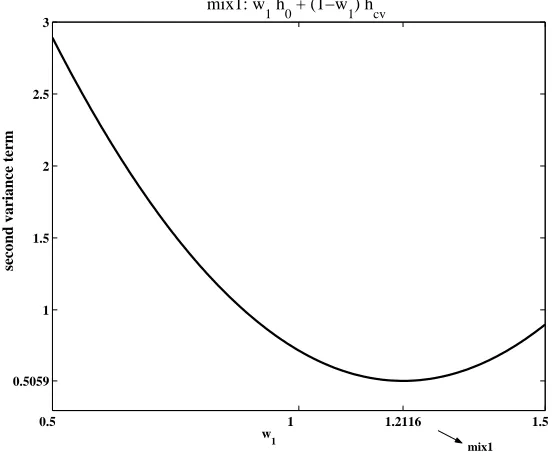
For given kernels K and L_j (j = 1, . . . , J) and a density f, we might explicitly calculate the components in the asymptotic variance in (11), for the just introduced class of bandwidth selectors (2), and also for the combinations (8). We look for good selectors, in the optimality sense of Hall and Johnstone (1992), i.e. bandwidths which, holding constant the first variance term in (11), have a small second term. Hall and Johnstone (1992) showed that an asymptotically achievable bandwidth exists where the second term is zero but they never pursued the issue any further and did not provide practical examples of such bandwidth selectors. In our search for good bandwidth selectors, we do for the first time provide a bandwidth selector with better asymptotic theory than the plug-in method, namely the optimal combination of plug-in (with weight w₁) and classical cross-validation. Figure 1 shows up to a factor the graphs of the resultant second variance term in (11) against the weight for the Epanechnikov kernel. We plot the noisy term in a wide range including negative weights to get optimality (as we argued in Section 1 because of the known negative correlation between them). And indeed the optimum is achieved by weighting the plug-in bandwidth with w₁ = 1.21 and cross-validation with w₂ = 1−w₁ = −0.21. Such an optimal combination yields a second term in (11) of 0.51C_f,K with C_f,K =

1

25R(K)−7/5μ−26/5(K)R(f)−3/5R(f). With 0.72Cf,K an asymptotically MISE optimal

the factor of the second term increases from 0.44 to 0.83. This gives an increase of expected ISE of up to 90 per cent. However, in the next section we will see that despite the excellent asymptotic properties these combined bandwidth selectors can show poor performance in finite samples.

0.5 1 1.2116 1.5

0.5059 1 1.5 2 2.5 3

w

1

mix1: w

1 h0 + (1−w1) hcv

second variance term

[image:16.612.160.438.173.402.2]

mix1

Figure 1: The factor 1₂ H(u)−J_j=1w_j

R(K)

R(Lj)

H_j(u)

₂

du of the second

compo-nent of the asymptotic variance in (11). The factor is plotted for the combination of

an asymptotical MISE optimal bandwidth with standard cross-validation. The density

estimator is calculated with an Epanechnikov kernel. For the combined bandwidth the

factor is equal to 1₂ [w₁H(u)−(1−w₁)4(K(u) +uK(u))]2du. The optimal value

is achieved by weighting the plug-in bandwidth with w₁ = 1.21.

In the following display we show the asymptotic variances of n3/10(h − h_ISE) or

standard cross-validation bandwidthh_CV, an asymptotical MISE optimal bandwidth

h_MISE, and two combinations of h_CV and h_MISE. The first combination h_mix1 is the optimal combination h_mix1 = 1.2116h_MISE−0.2116h_CV. The second one is the pragmatic average h_mix2 = 0.5h_MISE + 0.5h_CV. The asymptotic variances of these bandwidths are given for the Epanechnikov kernel by:

σ_OSCV2 = C_f,K

4R(K) V(f

₎

R(f)R(f) + 2.19

σ2_DO = C_f,K

4R(K) V(f

₎

R(f)R(f) + 2.19

σ_CV2 = C_f,K

4R(K) V(f

₎

R(f)R(f) + 7.42

σ_MISE2 = C_f,K

4R(K) V(f

₎

R(f)R(f) + 0.72

σ_mix12 = C_f,K

4R(K) V(f

₎

R(f)R(f) + 0.51

σ_mix22 = C_f,K

4R(K) V(f

₎

R(f)R(f) + 2.89

with C_f,K as above. For the quartic kernel we get the same expressions with the constants 2.19, 2.19, 7.42, 0.72, 0.51, 2.89 replaced by 1.46, 1.46, 5.87, 0.83, 0.44, 2.63.

in practice these differences become irrelevant. Now it is the numerical performance that matters.

5

Finite Sample Performance

The purpose of this section is to study the performance of the six bandwidths defined in Section 4 in finite samples, sometimes just of moderate size. As asymptotical MISE optimal bandwidth we use in the simulations a plug-in bandwidth h_{P I} as proposed by Sheather and Jones (1991); see also Park and Marron (1990). This plug-in band-widthis calculated from the asymptotic expression of the MISE-optimal bandwidth,

h_MISE ≈

R(K)

μ2₂(K)R(f)

1/5

n−1/5, whereR(K) andμ₂(K) are known, whereasR(f) has to be estimated. We now describe the estimatorR_f that we used. In a first step

we calculate a kernel density estimator of f with bandwidth g_p. For the choice of

g_p we take Silverman’s rule of thumb bandwidth for Gaussian kernels, see Silverman (1986, page 48). In our implementation the standard deviation of X is estimated by the minimum of two methods: the empirical standard deviation s_n and the in-terquartile range IR_X divided by 1.34, i.e. g_S = 1.06 min{IR_X1.34−1, s_n}n−1/5. As the quartic kernel K_Q comes close to the Epanechnikov but allows for estimating the second derivative, we normalizeg_S by the factors of the canonical kernel (Gaussian to quartic) and adjust for the slower rate (n−1/9) needed to estimate second derivatives, i.e.

g_p = g_S2.0362

0.7764 n

Next,

R_f =

f2− 1 ng_p5

K_Q2

to correct for the bias inherited by

f(x) = 1

ng_p3 n

i=1

K_Q

X_i−x g_p

.

In simulation studies not shown here this prior choice turned out to perform better than any of the many other plug-in estimators we tried, at least for the densities considered in our simulations.

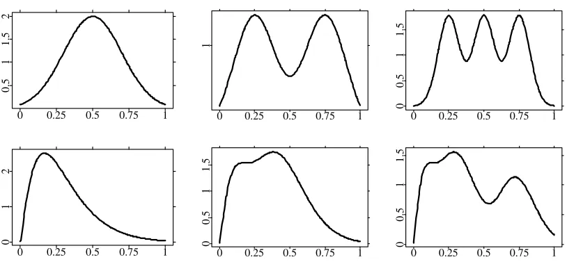
Our selected data generating processes are the following six densities (see also Figure 2):

1. a simple normal distribution, N(0.5,0.22),

2. a bimodal mixture of two normals which were N(0.35,0.12) and N(0.65,0.12), 3. a mixture of three normals, namelyN(0.25,0.0752),N(0.5,0.0752) andN(0.75,0.0752)

giving three clear modes,

4. a gamma distribution, Gamma(a, b) with b = 1.5, a = b2 applied on 5x with

x∈IR₊, i.e.

f(x) = 5 b

a

Γ(a)(5x)

a−1_e−5xb_,

5. a mixture of two gamma distributions, Gamma(a_j, b_j), j = 1,2 with a_j = b2_j,

b₁ = 1.5,b₂ = 3 applied on 6x, i.e.

f(x) = 6 2

2

j=1

ba_jj

Γ(a_j)(6x)

aj−1_e−6xbj

6. and a mixture of three gamma distributions, Gamma(a_j, b_j), j = 1, ...,3 with

a_j = b2_j, b₁ = 1.5, b₂ = 3, and b₃ = 6 applied on 8x giving two bumps and one plateau.

0 0.25 0.5 0.75 1

0.5

1

1.5

2

0 0.25 0.5 0.75 1

0

1

2

0 0.25 0.5 0.75 1

1

0 0.25 0.5 0.75 1

0

0.5

1

1.5

0 0.25 0.5 0.75 1

0

0.5

1

1.5

0 0.25 0.5 0.75 1

0

0.5

1

[image:20.612.104.511.164.359.2]

1.5

Figure 2: The six data generating densities: Designs 1 to 6 from the upper left to the lower right.

Our set of densities contains density functions with one, two or three modes, some being asymmetric. They all have exponentially falling tails, because otherwise one has to work with boundary correcting kernels. The main mass is always in [0,1]. We use the following measures to summarize the stochastic performance of the bandwidth selectors:

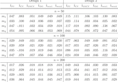
m₁ = mean(ISE(h)), m₂ = std(ISE(h))

m₃ = mean(h−h_ISE), m₄ = std(h−h_ISE).

onesided cross-validation presented here is the left-onesided. The original simulation study comprised more designs, kernels, and samples sizes, but the findings were all in line with the here presented results. The results given in Tables 1 to 3 and 4 were calculated from 250 repetitions for each model and each sample size. Note that the standard deviations of the Monte Carlos means m₁ and m₃ in Tables 1-4 are simply

m₂/√250 ≈0.06 m₂ and m₄/√250, respectively.

Design 1 Design 2

hP I hCV hOSCV hDO hmix1 hmix2 hP I hCV hOSCV hDO hmix1 hmix2 n= 50

m1 .047 .083 .051 .049 .049 .049 .115 .111 .106 .103 .130 .083

m2 .033 .100 .043 .036 .033 .037 .023 .114 .033 .034 .025 .032 m3 .047 -.011 .032 .034 .059 .018 .117 .018 .092 .090 .138 .067

m4 .054 .095 .066 .064 .053 .069 .044 .078 .076 .072 .047 .054 n= 100

m1 .029 .049 .031 .030 .031 .030 .077 .063 .049 .049 .091 .052 m2 .020 .059 .021 .020 .021 .020 .017 .055 .027 .026 .017 .024 m3 .035 -.016 .019 .019 .046 .010 .098 .010 .035 .035 .116 .054

m4 .047 .078 .057 .056 .046 .058 .024 .059 .048 .046 .022 .039 n= 200

m1 .017 .026 .018 .018 .018 .018 .049 .043 .034 .030 .059 .033 m2 .012 .029 .014 .014 .012 .013 .013 .054 .041 .017 .012 .016 m3 .029 -.005 .010 .011 .036 .012 .075 .000 .014 .015 .091 .037

[image:21.612.100.497.231.507.2]

m4 .036 .064 .045 .044 .045 .047 .019 .044 .035 .031 .017 .029

Table 1: Criteria m₁, m₂, m₃ and m₄ for Designs 1 and 2.

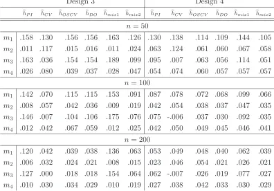
Design 3 Design 4

hP I hCV hOSCV hDO hmix1 hmix2 hP I hCV hOSCV hDO hmix1 hmix2 n= 50

m1 .158 .130 .156 .156 .163 .126 .130 .138 .114 .109 .144 .105

m2 .011 .117 .015 .016 .011 .024 .063 .124 .061 .060 .067 .058 m3 .163 .036 .154 .154 .189 .099 .095 .007 .063 .056 .114 .051

m4 .026 .080 .039 .037 .028 .047 .054 .074 .060 .057 .057 .057 n= 100

m1 .142 .070 .115 .115 .153 .091 .087 .078 .072 .068 .099 .066 m2 .008 .057 .042 .036 .009 .019 .042 .054 .038 .037 .047 .035 m3 .146 .007 .104 .106 .175 .076 .075 -.006 .037 .030 .092 .035

m4 .012 .042 .067 .059 .012 .025 .042 .050 .049 .045 .046 .041 n= 200

m1 .120 .042 .039 .038 .136 .063 .053 .049 .048 .040 .062 .039 m2 .006 .032 .024 .021 .008 .015 .023 .046 .054 .021 .026 .021 m3 .127 .000 .018 .018 .154 .064 .062 -.007 .026 .019 .077 .027

[image:22.612.99.495.58.334.2]

m4 .010 .030 .034 .029 .010 .019 .027 .038 .042 .033 .030 .029

Table 2: Criteria m₁, m₂, m₃ and m₄ for Designs 3 and 4.

2 and 4 as harder problems and Design 3 as a very hard estimation problem. For Designs 5 and 6 the difficulty depends on the sample size and it increases with sample size. We conjecture that for these two designs accurate estimation of the small wiggles of the underlying density is impossible for small sample sizes but it requires a fine tuning of the bandwidths for larger sample sizes.

The cross-validation bandwidth h_CV and the asymptotically optimal combination

h_mix1 of h_CV and h_{P I} show the poorest behaviour in the simulations. They have in all designs and for all sample sizes the largest expected ISE m₁. For h_CV this is mainly caused by the large variance of this bandwidth selector, see the outcomes of

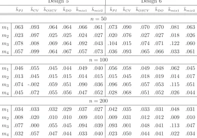
Design 5 Design 6

hP I hCV hOSCV hDO hmix1 hmix2 hP I hCV hOSCV hDO hmix1 hmix2 n= 50

m1 .063 .093 .064 .064 .066 .061 .073 .090 .070 .070 .081 .063

m2 .023 .097 .025 .025 .024 .027 .020 .076 .027 .027 .018 .026 m3 .078 .008 .069 .064 .092 .043 .104 .015 .074 .071 .122 .060

m4 .057 .099 .064 .067 .057 .073 .036 .093 .065 .066 .033 .061 n= 100

m1 .046 .055 .045 .044 .049 .040 .056 .058 .049 .048 .062 .045 m2 .013 .045 .015 .015 .014 .015 .015 .045 .018 .019 .014 .017 m3 .074 -.002 .059 .051 .090 .036 .096 .005 .057 .053 .115 .051

m4 .045 .072 .055 .056 .047 .052 .028 .068 .051 .052 .026 .044 n= 200

m1 .034 .033 .032 .029 .037 .027 .042 .035 .033 .031 .048 .031 m2 .008 .020 .010 .010 .009 .010 .009 .031 .012 .012 .009 .010 m3 .077 .000 .055 .045 .094 .039 .093 .001 .048 .041 .113 .047

[image:23.612.102.497.58.334.2]

m4 .032 .057 .047 .044 .033 .040 .023 .050 .044 .041 .022 .034

Table 3: Criteria m₁, m₂, m₃ and m₄ for designs 5 and 6.

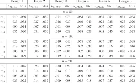
understand the poor behaviour of h_mix1 we have carried out additional simulations where we replacedh_{P I} in the definition ofh_mix1byh_MISE. In Table 4 we compare the theoretical bandwidth h_mix1 = 1.2116h_MISE −0.2116h_CV with the MISE minimizer

Design 1 Design 2 Design 3 Design 4 Design 5 Design 6

hMISE Mix1 hMISE Mix1 hMISE Mix1 hMISE Mix1 hMISE Mix1 hMISE Mix1

n= 50

m1 .040 .039 .059 .059 .074 .075 .083 .083 .055 .054 .054 .053 m2 .033 .032 .037 .039 .036 .039 .049 .049 .025 .025 .026 .026

m3 .009 .014 -.007 -.012 -.001 -.008 .007 .007 .007 .007 .006 .004 m4 .035 .030 .034 .036 .026 .028 .028 .026 .048 .045 .036 .033

n= 100

m1 .026 .025 .036 .035 .046 .046 .055 .055 .037 .037 .039 .038 m2 .019 .019 .020 .020 .025 .025 .032 .032 .015 .015 .016 .016

m3 .003 .007 .006 .005 -.002 -.004 .002 .004 .000 .000 -.003 -.004 m4 .032 .029 .017 .015 .012 .012 .024 .023 .038 .039 .028 .026

n= 200

m1 .016 .015 .025 .024 .030 .029 .034 .034 .024 .024 .025 .025

[image:24.612.86.537.57.334.2]

m2 .011 .011 .014 .014 .013 .013 .019 .019 .010 .010 .010 .010 m3 .003 .005 .005 .006 -.001 -.002 .006 .008 .003 .003 -.002 -.003 m4 .026 .023 .014 .012 .009 .008 .018 .018 .027 .027 .023 .022

Table 4: Values of m₁, m₂, m₃ and m₄ for h_MISE and h_mix1.

only marginally better - measured by m₁ and m₂ - than one-sided cross-validation on most of the designs. But for the asymmetric density design 4 it is clearly better. For the bimodal density 2 and the trimodal density 3h_mix2 outperformsh_DO whereas for the trimodal density with larger sample size 200,h_mix2 has an increase in the expected ISE of 66 %. The simplicity of do-validation, no need of the choice of pilot band-width and its overall excellent performance in this simulation make do-validation a very promising bandwidth selector. To conclude again from this study, classical cross-validation is a crystal clear loser of this test. It is almost unbiased and that is good, but volatility just kills its overall performance. Therefore we suggest that practition-ers leave classical cross-validation and start to use do-validation. Do-validation is just another cross-validation technique, it is relatively simple to carry out, it is well defined without ambiguities and does not need complicated pilot estimation.

6

Conclusions

simple procedure that does not need any pilot estimation and that is to implement as simple as classical cross-validation.

principles and beats plug-in asymptotically.

We consider pilot-free MISE optimal estimation and pilot-free MISE near optimal estimation an important area of future research in kernel density bandwidth selec-tion. The key research element of pilot-free MISE optimal estimation seems to be to determine a practical solution to the trade off between the two entering components in the indirect kernel. The discussion on pilot-free MISE optimal estimation also gives us some intuition to why onesided cross-validation and do-validation work so well. While both of these two latter methods are practical and easy to implement, they are a first step towards a pilot-free MISE optimal estimator. In the first step it does blow up variance to some extent while keeping bias relatively stable. However, it does not bother to optimize this idea asymptotically by blowing up the variance indefinitely in the indirect step with all the practical problems this implies. One-sided cross-validation and do-validation are practical and pragmatic first steps towards pi-lot free MISE optimal estimation, but with easy stable implementations that work extremely well in practice.

Appendix

ForL=K and L=L_j (j = 1, . . . , J) we use the following notation. Define Δ_L(h) = f_L,h(x)−f(x)

₂

dx (ISE),

ML(h) = E [ΔL(h)] (MISE),

DL(h) = ΔL(h)−ML(h), δ_L(h) = 2

f(x)f_L,h(x)dx−2n−1 n

i=1

f_L,h(X_i).

Here f_L,h(x) denotes the kernel density estimator with bandwidth h and kernel L. Define

h_L,0 = arg min

h ML(h), h_L,0 = arg min

h ΔL(h), h_L,c = arg min

h

Δ_L(h) +δ_L(h)−

f(x)2dx

(CV-bandwidths).

Under our conditions it holds that

h_L,0 =

R(L)

μ2₂(L)R(f)

_1/5

n−1/5+on−3/10.

Proceeding as in Hall and Marron (1987) one can show that for L=K, L₁, . . . , L_J:

h_L,0−h_L,0 = −M_L(h_L,0)−1D_L(h_L,0) +o_pn−3/10, (14)

h_L,c−h_L,0 = −M_L(h_L,0)−1(D_L(h_L,0) +δ_L(h_L,0)) +o_pn−3/10. (15)

to note that:

M_L(h_L,0) = 0, (16) Δ_L(h_L,0) = 0, (17) Δ_L (h_L,c) +δ_L(h_L,c) = 0. (18) Equation (16) still holds under Assumption (A1). We now argue that equations (17)-(18) remain to hold under Assumption (A1) if the right hand sides of the equations are replaced byO_P(n−2h−2) =O_P(n−8/5). To see this one has to note that for a finite set T ⊂ IR the following event has probability zero: there exists an h > 0 such that for two pairs (i, j) and (i, j) it holds thath−1(X_i−X_j)∈T andh−1(X_i−X_j)∈T.

This statement follows easily because the observations have a density. Thus we have that with probability equal to one for all h >0 at most for one pair (X_i, X_j) it holds that h−1(X_i−X_j) lies on a point where the kernel L is not differentiable. Consider now Δ_L(h_L,0) and Δ_L(h_L,c) + δ_L(h_L,c). These are double sums over indices (i, j). Using our considerations we get that with probability one the left- and right-sided derivatives of the summands differ only for at most one double index (i, j). Now one uses a simple bound for the one-sided derivatives of the summands that is of the order

O(n−2h−2). Thus we have that (17)-(18) hold with the right hand sides replaced by

O_P(n−8/5). One can check that this change does not affect the lines of proof used in Hall and Marron (1987).

One can show that for L=K, L₁, . . . , L_J with h=h_L,0: D_L(h) = n−2

i<j

W_L,i,j+n−1 i

with W_L,i,j∗ =−h−2H_L

X_i−X_j h

,

H_L(u) = 2

L(u+v)L(v)dv+2

L(−u+v)L(v)dv+2

L(u+v)vL(v)dv+2

L(−u+v)vL(v)dv,

W_L,i,j = W_L,i,j∗ −EW_L,i,j∗ |X_i−EW_L,i,j∗ |X_j+ EW_L,i,j∗ , W_L,i∗ = 2h

μ2₂(L)f(X_i), W_L,i = W_L,i∗ −EW_L,i∗ .

For a proof of (19) note that D_L(h) is a U-statistic with quadratic terms W_L,i,j∗ . We replace W_L,i,j∗ by W_L,i,j to have that E [W_L,i,j|X_i] = E [W_L,i,j|X_j] = 0, a.s. The remaining terms are sums of independent mean zero variables. By standard smoothing theory expansions it can be shown that these summands are asymptotically equivalent toW_L,i.

Furthermore, we have for h=h_L,0 and L=L₁, . . . , L_J δ_L (h) =n−2

i<j

V_L,i,j−n−1 i

W_L,i+o_pn−7/10

with V_L,i,j∗ =h−2G_L

X_i−X_j h

, G_L(u) = 2 [L(u) +uL(u) +L(−u)−uL(−u)].

We now use

h_K,0 =

R(K)

μ2₂(K)

μ2₂(L_j)

R(L_j)

_1/5

h_Lj,0+on−3/10

=

R(K)

μ2₂(K)

μ2₂(L_j)

R(L_j)

1/5

This gives together with the above expansions:

h−h_ISE =

J

j=1

w_j

R(K)

μ2₂(K)

μ2₂(L_j)

R(L_j)

1/5

(h_Lj,c−h_Lj,0)−(h_ISE −h_K,0) +on−3/10

=

J

j=1

w_jM_Lj(h_Lj,0)−1

R(K)

μ2₂(K)

μ2₂(L_j)

R(L_j)

_1/5

−n−2 i<k

W_Lj,i,k+V_Lj,i,k

−M_K(h_MISE)−1

−n−2 i<k

W_K,i,k−n−1 i

W_K,i

+o_pn−3/10.(20) Now

M_L(h_L,0) = 2R(L)

nh3_L,0 + 3μ

2

2(L)R(f)h2L,0+o

n−2/5

= n−2/55R(L)2/5R(f)3/5μ6₂/5(L) +on−3/5

With the above expansion this gives

h−h_ISE = M_K(h_MISE)−1n−1 i

W_K,i

+M_K(h_MISE)−1n−2 i<k

Z_ik+o_pn−3/10

with Z_ik =Z_ik∗ −E [Z_ik∗|X_i]−E [Z_ik∗|X_j] + E [Z_ik∗],

Z_ik∗ = −h−_0,K2 H_K

X_i−X_k h_MISE − J j=1 w_j

R(K)

R(L_j) HLj

X_i−X_k h_0,Lj

+G_Lj

X_i−X_k h_0,Lj

Note that we collect in the definition ofZ_ik∗ all quadratic terms in the right hand side of (20). These are the terms: −n−2w_jM_L

j(hLj,0)−1

R(K)

μ2 2(K)

μ2 2(Lj)

R(Lj)

_1/5

W_Lj,i,k,−n−2w_j M_Lj(h_Lj,0)−1

R(K)

μ2 2(K)

μ2 2(Lj)

R(Lj)

_1/5

V_Lj,i,k and n−2M_K(h_MISE)−1W_K,i,k.

References

Ahmad, I.A. and Ran, I.S., 2004, Data based bandwidth selection in kernel density estimation with parametric start via kernel contrasts,Journal of Nonparametric

Statistics. 16, 841–877.

Bowman, A., 1984, An alternative method of cross-validation for the smoothing of density estimates. Biometrika, 71, 353–360.

Cao, R., 1993, Bootstrapping the Mean Integrated Squared Error, Journal of

Mul-tivariate Analysis, 45, 137–160.

Chaudhuri, P. and Marron, J.S., 1999, SiZer for Exploration of Structures in Curves.

Journal of the American Statistical Association, 94, 807–823.

Cheng, M.Y., 1997a, Boundary-aware estimators of integrated squared density deriva-tives. Journal of the Royal Statistical Society Ser. B,50, 191–203.

Cheng, M.Y., 1997b, A bandwidth selector for local linear density estimators. The

Annals of Statistics, 25, 1001–1013.

Chiu, S.T., 1991, Bandwidth selection for kernel density estimation. The Annals of

Statistics, 19, 1883–1905.

Godtliebsen, F.; Marron, J.S. and Chaudhuri, P., 2002, Significance in Scale Space for Bivariate Density Estimation. Journal of Computational and Graphical

H¨ardle, W., Hall, P. and Marron, J.S., 1988, How far are automatically chosen regression smoothing parameters from their optimum?. Journal of the American

Statistical Association, 83, 86–99.

Hall, P., 1984, Central Limit Theorem for Integrated Square Error of Multivariate Nonparametric Density Estimators. Journal of the Multivariate Analysis, 14, 1–16.

Hall, P. and Johnstone, I., 1992, Empirical Functionals and Efficient Smoothing Parameter Selection. Journal of the Royal Statistical Society B, 54 (2), 475– 530.

Hall, P. and Marron, J.S., 1987, Extent to which Least-Squares Cross-Validation Minimises Integrated Square Error in Nonparametric Density Estimation.

Prob-ability Theory and Related Fields, 74, 567–581.

Hall, P., Marron, J.S. and Park, B., 1992, Smoothed cross-validation. Probability

Theory and Related Fields, 92, 1–20.

Hanning, J. and Marron, J.S., 2006, Advanced Distribution Theory for SiZer.

Jour-nal of the American Statistical Association, 101, 484–499.

Hart, J.D., and Lee, C.-L., 2005, Robustness of one-sided cross-validation to auto-correlation. Journal of Multivariate Statistics, 92, 77–96.

Hart, J.D. and Yi, S., 1998, One-Sided Cross-Validation. Journal of the American

Jones, M.C., 1993, Simple boundary correction in kernel density estimation.

Statis-tics and Computing, 3, 135–146.

Loader, C.R., 1999, Bandwidth selection: classical or plug-in. The Annals of Statis-tics, 27, 415–438.

Mart´ınez-Miranda, M.D., Nielsen, J. and Sperlich, S., 2009, One sided cross-validation for density estimation with an application to operational risk. In ”Operational Risk Towards Basel III: Best Practices and Issues in Modelling. Management

and Regulation, ed. G.N. Gregoriou; John Wiley and Sons, Hoboken, New

Jer-sey.

Park, B.U. and Marron, J.S., 1990, Comparison of Data-Driven Bandwidth Selectors.

Journal of the American Statistical Association, 85, 66–72.

Rudemo, M., 1982, Empirical choice of histograms and kernel density estimators.

Scandinavian Journal of Statistics, 9, 65–78.

Savchuk, O.Y., Hart, J.D., and Sheather S.J., 2010a, Indirect cross-validation for Density Estimation. Submitted to Journal of the American Statistical

Associ-ation, 105, 415–423.

Savchuk, O.Y., Hart, J.D., and Sheather S.J., 2010b, An empirical study of indirect cross-validation for Density Estimation. IMS Lecture Notes - Festschrift for Tom Hettmansperger.

Sheather, S.J. and Jones, M.C., 1991, A reliable data-based bandwidth selection method for kernel density estimation. Journal of the Royal Statistical Society, Ser. B, 53, 683–690.

Silverman, B. W., 1986, Density Estimation. London: Chapman and Hall.

˙Zychaluk, K. and Patil, P.N., 2008, A cross-validation method for data with ties in kernel density estimation. Annals of the Institute of Statistical Mathematics,