A Laplacian-based algorithm for non-isothermal atomistic-continuum
hybrid simulation of micro and nano-flows
q
Alessio Alexiadis
a,⇑, Duncan A. Lockerby
a, Matthew K. Borg
b, Jason M. Reese
b aSchool of Engineering, University of Warwick, Coventry CV4 7AL, United Kingdom b
Mechanical & Aerospace Engineering, University of Strathclyde, Glasgow G1 1XJ, United Kingdom
a r t i c l e
i n f o
Article history:Received 17 January 2013
Received in revised form 17 April 2013 Accepted 29 May 2013
Available online 6 June 2013
Keywords:
Atomistic-continuum hybrid modelling Molecular dynamics
Fluid dynamics
a b s t r a c t
We propose a new hybrid algorithm for incompressible micro and nanoflows that applies to non-isother-mal steady-state flows and does not require the calculation of the Irving–Kirkwood stress tensor or heat flux vector. The method is validated by simulating the flow in a channel under the effect of a gravity-like force with bounding walls at two different temperatures and velocities. The model shows very accurate results compared to benchmark full MD simulations. In the temperature results, in particular, the contri-bution of viscous dissipation is correctly evaluated.
Ó2013 The Authors. Published by Elsevier B.V. All rights reserved.
1. Introduction
Current developments in micro and nanofluidics have created the need for new computational methods that can concurrently and efficiently handle different time and length scales. At these scales in fact the continuum-fluid hypothesis loses its validity and the behaviour of the fluid should be calculated, at least in theory, from the (averaged) motion of its constitutive molecules. In prac-tice, however, most of the time the continuum formulation can still be employed to describe the overall behaviour of the fluid, but certain ‘adjustments’ must be introduced. The standard no-slip boundary conditions, for instance, cannot always be employed in microflows, while confinement in nanochannels creates anisotro-pies in a fluid’s density and alterations of the molecular distribution function, which, in turn, affect all the macroscopic properties of the fluid. This phenomenon has been clearly demonstrated for water in carbon nanotubes[3,4,5,6,28,29], where self-diffusivity, hydrogen bonding, freezing point, viscosity, etc. are not only very different from those of bulk water, but also non-uniformly distributed in the nanotube. If we consider, for instance, the case of transport properties (e.g. viscosity, diffusivity, and thermal conductivity), the attempt to provide a classical correlation of the type flux =f(gradient) (viz. flux of momentum, heat or mass as a function of, respectively, velocity, temperature or concentration gradient)
would fail because the result would depend not only on the fluid characteristics but also on the size and the geometry of the nanochannel. There are even some macroscopic cases that are difficult to treat with traditional continuum modelling and would benefit from an atomistic treatment. Complex polymeric fluids, for instance, can be strongly non-Newtonian and the stress/velocity relation cannot always be tabulated.
In all of these cases, a full molecular approach such as molecular dynamics (MD) would provide a better picture of the fluid’s behav-iour. Despite the recent advances in computer hardware and soft-ware, however, molecular simulations cannot yet handle the large number of atoms involved in many micro and nanofluidic applica-tions. In order to tackle this problem, various atomistic-continuum hybrid (ACH) models have been recently proposed (see[27]for a review). The fluid, depending on the model, is treated globally or partially as a continuum, and described by the Navier–Stokes equa-tions; in certain specific regions, however, molecular dynamics is employed.
One practical advantage of these hybrid methods consists in the fact that, independently, both the continuum and the atomistic numerical parts have been extensively developed in the last dec-ades, and researchers can now take advantage of the many acces-sible computational fluid dynamics (CFD) and molecular dynamics (MD) codes. Current research in the field therefore focuses on the coupling between the continuum and the atomistic solvers.
There are various ACH methods available in the literature (see [27] for a review), which can be classified according to the way they exchange information between the continuum and atomistic solvers. Each of these methods has specific advantages and disad-vantages according to the particular application chosen. Here, we
0045-7825/$ - see front matterÓ2013 The Authors. Published by Elsevier B.V. All rights reserved.
http://dx.doi.org/10.1016/j.cma.2013.05.020
q
This is an open-access article distributed under the terms of the Creative Commons Attribution License, which permits unrestricted use, distribution, and reproduction in any medium, provided the original author and source are credited.
⇑ Corresponding author.
E-mail address:[email protected](A. Alexiadis).
Contents lists available atSciVerse ScienceDirect
Comput. Methods Appl. Mech. Engrg.
focus on the approach known as the heterogeneous multiscale
method (HMM) [31] or, alternatively, as point-wise coupling
(PWC)[10]. These hybrid methods are particularly useful in the case of the so-called ‘type B’ problems [31], which require the determination of first-principle-based closure terms in the consti-tutive parts of the macroscopic momentum equation. In our case, for instance, this means that certain specific elements of the Navier–Stokes equations (e.g. shear stress) are derived directly from atomistic calculations.
[image:2.595.353.499.630.739.2]The general approach of the HMM/PWC is the following
[31,10,13]. Let us assume that the value of a microscopic variable
u(streaming velocity) can be determined by means of a microscale model (e.g. molecular dynamics). We are not interested in the microscopic details ofu, but rather a coarse-grained representation U(the macroscopic velocity field), which comes from the solution of the Navier–Stokes equation written in the form
@U
@t ¼
1
q
r
Tþg; ð1Þwheretis the time,
q
is the density,gis the external force per unitmass andTis the momentum flux defined as
T¼
q
UUþpIs
; ð2Þwherepis the pressure,Ithe identity matrix and
s
the shear stress. In traditional continuum modelling, an empirical relationship be-tween the shear stress and the strain rate is introduced in order to close Eq. (2)and, therefore, Eq. (1). In HMM, the microscopic model provides all the information necessary to determineT. This is usually done by means of the Irving–Kirkwood (IK) equation[18])Tðr;tÞ ¼1
V X
i
mi
v
iv
iþ1 2
X
i;j
rijOijfijjri¼r
" #
; ð3Þ
wheremiis the mass of moleculei,rithe position,viis the velocity, fijis the force acting on moleculeiby thejmolecule and the
oper-atorOijis given by
Oij1
1 2!rij
@ @rþ þ
1
n! rij
@ @r
n1
þ ð4Þ
In practice, the calculation of theOijterm can be rather complicated
for non-equilibrium simulations. Ren and E[31]partially simplify this task by calculating the average flux and employing a 2D mod-ification of the Lees–Edwards shear boundary conditions. This type of computational cell is periodic and changes its shape during the simulation in such a way as to produce a specific velocity gradient in the flow. From this gradient, the momentum flux can be calcu-lated by Eq.(3)and introduced into Eq.(1).
In this paper, however, we prefer the simpler ‘framed’ cell em-ployed by Hadjiconstantinou and Patera[16], where the shear stress is generated by constraining the velocity in a ‘frame’ rather than by modifying the shape of the box. The framed cell is periodic, but we cannot simply calculate the average stress in the whole box because the presence of an external buffer would produce spurious results. We need the local stress in the core region, but this complicates theOijterm in Eq.(3). There are other methods to calculate the stress
tensor such as the method of planes [32], the volume-average approach[26,14], or the method derived from the Schweitz virial relation[25], but, in general, we must choose between a compli-cated computational cell (i.e. Lees–Edwards cell) and simplifying the calculation of the momentum flux, or a simple cell (i.e. framed cell) and complicating the calculation of the momentum flux. The new method we propose here does not need the direct calculation of the flux, so it avoids this issue altogether: we can use the framed cell and, at the same time, avoid the calculation of the IK equation. Our approach, furthermore, works for steady-state systems. In one of the first hybrid methods proposed for the case of dense
fluids, the Domain Decomposition Method (DDM), the transient case was more challenging than the steady-state because the con-tinuum time-step was partially related to the atomistic one (see [27] for details). In its original formulation [31], however, the HMM cannot be used for steady-state flows, since, if in Eq.(1) the time derivative vanishes, U disappears and the continuum solution cannot be calculated. Steady-state solutions, of course, can always be obtained as limiting cases of a time-implicit simula-tion, but this option is not optimal when long transient periods are involved. This circumstance can limit the applicability of the meth-od, since many micro and nanofluidic practical applications work at steady state[1].
The other benefit of the method we propose here is that it can be easily extended to non-isothermal flows and, in this arti-cle, momentum and heat transfer are actually handled together. Before hybrid models can express their full potential for engi-neering applications, they must be able to manage the whole spectrum of transport phenomena (i.e. momentum, heat and mass). While there is one study including heat transport in
the DDM [24], the HMM is, for the moment, limited only to
momentum transfer (diffusive mass transfer is still missing in both formulations). We must also consider that, at the molecu-lar scale, heat and momentum transport are connected, which usually does not emerge in macroscopic flows at low Mach number. Isothermality, in fact, is a common assumption in engi-neering flows where heat is neither generated (e.g. from nuclear or chemical reactions) nor externally introduced (e.g. walls at a different temperature from the fluid). At the microscale and especially at the nanoscale, however, the relative importance of viscous dissipation increases [21] and, therefore, a velocity gradient can result in a non-negligible amount of internally gen-erated heat. Momentum and heat transport are consequently coupled and must be solved together.
This paper is organized as follows. First, we give a general over-view of how the atomistic-continuum hybrid algorithm works. Second, we describe the MD box we use for our simulation and how velocity and temperature are constrained in order to be con-sistent with the continuum solution. Third, we reformulate the coupling in such a way that the calculation of the IK fluxes is avoided. Finally, we validate the method against a benchmark case: non-isothermal channel flow.
2. Algorithm’s overview
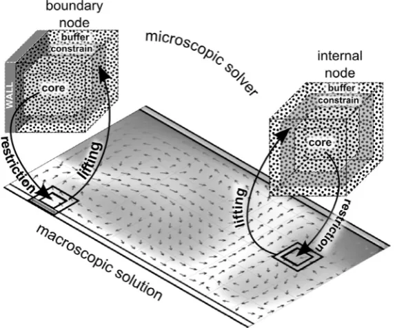
Hybrid models for fluid simulations such as HMM or PWC gen-erally work as illustrated inFig. 1. The cyclic scheme is composed of the following four steps, which are repeated during the calcula-tion until convergence. (Here we assume that the ‘locacalcula-tion’ of every MD simulation corresponds to one node on the continuum grid.)
Step 1. Macroscopic solver: the continuum solution is calculated at the N discretization nodes of the macroscopic domain.
Step 2. Lifting1: knowing the macroscopic solution at the nodes, we can determine N sets of boundary condition to be applied to the microscopic solver.
Step 3. Microscopic solvers: N molecular dynamics simulations are run.
Step 4. Restriction: the molecular results are processed in order to extract the information required to update the macro-scopic solver and start a new cycle.
Steps 1 and 3 are respectively the ‘pure’ continuum and molec-ular models; good general references, in this case, are respectively Landau and Lifshitz[22]and Allen and Tildesley[8]. Steps 2 and 4, however, are specific to hybrid models; in practice, each of these can be seen as an interface which regulates the exchange of infor-mation between the two solvers. The type of inforinfor-mation, and how it is extracted from one model and introduced into the other, is precisely what characterizes a specific hybrid approach. In Sections
3 and 4we discuss Steps 2 and 4 of our approach.
In the following sections we generally use lowercase letters (u,r, z, etc.) for the fluid variables related to the micro subdomain and uppercase letters to indicate the corresponding macroscopic variables (U,R, Z, etc.). The only exception is the temperature T; since the lowercasetis used for time, the temperature for the mi-cro-simulations is indicated with the Greek letter#. For consis-tency with the units used in our MD code, all results are presented in reduced/normalized units as described inAppendix A.
3. The framed computational cell
Consistency between the microscopic and the macroscopic do-mains imposes certain conditions (e.g. streaming velocity, density and temperature) at the boundaries of the MD cell. If we think of the MD cell as a small window embedded into the macroscopic do-main as inFig. 2, we understand that, in the region where the two domains are ‘glued’ together, the outcome of the two models should match. Let us assume, for instance, that, as in the HMM,
the first-principle data the continuum model requires is the momentum flux calculated from the MD simulation and then passed to the macroscopic solver. The value of the momentum flux depends on the velocity gradient; this information is contained in the continuum domain, which, therefore, must be passed to the microscopic solver as a boundary condition. In order to achieve this goal, we use the ‘framed’ cell proposed by Hadjiconstantinou and Patera[16](seeFig. 2). Both the MD cells and the continuum do-main are, of course, three-dimensional, but in order to make the picture simpler a two-dimensional macroscopic flow is illustrated
inFig. 2. The internal region of the cellthe ‘core’is the region
where the MD information is extracted and transmitted to the macroscopic model. The grey area is the ‘frame’ or ‘constrained re-gion’; the region where the two models are coupled together and where the information from the macroscopic model is imposed on the microscopic model. The external region surrounding the frame is the ‘buffer’, which does not play any role in the exchange of information between the solvers but it allows the solution to re-lax between the external boundaries of the box and the frame.
Various ways of constraining the velocity in the MD simulation have been proposed. There is no unanimous opinion on what is the best option (see[27]for a review). Here, we use a simple velocity-shifting/velocity-rescaling technique. The frame is divided into bins and, at each time step, the molecular velocity distribution in the bin is rescaled and shifted so that the streaming velocity and temperature of the molecules contained in the bins match those of the continuum domain. The streaming velocity is defined as
u¼
P imi
v
i Pimi
; ð5Þ
and the temperature
#¼
P
imiðu
v
iÞ2 kBNm; ð6Þ
wherekBis the Boltzmann constant andNmthe number of degrees
of freedom of the system.
In Hadjiconstantinou and Patera [16], the constraint was
[image:3.595.158.445.68.306.2]achieved by using a ‘Maxwell Demon’ approach. In our case, how-ever, we find that the velocity-shifting/velocity-rescaling strategy Fig. 2.Schematic representation of the macro-to-micro (lifting) and micro-to-macro (restriction) exchange of information for a boundary node and an internal node.
1
We borrow the terms ‘lifting’ and ‘restriction’ from the ‘equation free’ literature
provides a smoother transition, especially for temperature profiles, between the frame and the core region. More details on this type of cell can be found in Drikakis and Asproulis[11].
The role of the buffer in the MD sub-domain is also important. There are, in fact, two types of conceptually different boundary conditions in the cell and they should not be confused.2The first conditions are the velocity and temperature profiles coming from the continuum domain. These are fundamental to the physics of the problem and are imposed in the frame. The second conditions are the external boundaries of the computational box. Since any molecular dynamic simulation is carried out in a computational box, a set of rules must be established to determine what happens if a molecule crosses the boundaries of the box. In the present case, these boundary conditions are only needed to contain all the mole-cules within the computational box and the molemole-cules in the buffer are not considered in the calculation of any property transferred to the macroscopic solver.
We can restrain the molecules in the box by using periodic boundary conditions or artificial walls (force fields). Generally, we use periodic boundary conditions because, in this way, the pro-files are smoother and, therefore, the thickness of the buffer region can be smaller. However, this solution is only possible in the inter-nal nodes of the macroscopic domain. In the boundary nodes,3 where at least one of the cell faces is a boundary (e.g. solid wall, interface between two fluids, etc.), periodic boundary conditions cannot be used in the direction normal to the boundary. In this case, we need to use a force field or an artificial wall to confine the mol-ecules. Here we use a reflecting wall, which bounces back the mole-cules in a mirror-like fashion when they cross the boundary.Fig. 3 shows the temperature (#), the streaming velocity (ux) and the
den-sity4(
q
0) profiles in an internal and in a boundary node reported in reduced units.InFig. 3, we show a version of the ‘framed’ cell that is modified
for channel flows. The streaming velocity simplifies touxand the
other components are zero. Since, in this case, the flow in the x andydirection is symmetric, the framed cell can be substituted by the ‘layered’ cell illustrated on the right side ofFig. 3. If the node is on the boundary, on one side we have the wall molecules but no frame and no buffer; on the other side, we have the constrained and the buffer ‘slices’, as before.
InFig. 3(a) (for bulk node), the sudden jumps in the measured
values between the constrained and buffer region bins are due to the fact that the cell is periodic and, consequently, the two buffer ‘slices’ are contiguous.Fig. 3(b) (for a wall boundary node) shows that on the non-periodic boundaries the density oscillates. This is due to molecular stratification and it is the correct behaviour in the proximity of a wall. In our boundary nodes, however, only one side has a real wall; the other side has an artificial wall that is only needed to confine the molecules. On the artificial wall, therefore, the oscillations are not physical and must be excluded from the core region. Sometimes, however, it is not easy to estab-lish beforehand how deep into the cell the effects of these oscilla-tions propagate. For this reason, the buffer of the boundary nodes should normally be larger. The method we propose (see Section4) handles the boundary and the internal nodes differently. At the boundary nodes, all the necessary coupling information is not ex-tracted from the core, but from bins close to the wall.5Therefore,
the only thing we have to pay attention to is that the perturbations generated by the two walls (the real and the artificial) do not over-lap. With this method, there is no need to use larger cells near the wall. On the contrary, in this region, we can even use smaller cells.
4. Coupling with the macroscopic solver
After the MD simulations are completed, we need to extract information from the core of the cell and pass it to the macroscopic model.
In Ren and E[31], the momentum flux was calculated by means of the IK equation and then introduced into Eq.(1). Our method, in-stead, is based on the value of the Laplacian of the streaming veloc-ityUand, since we consider non-isothermal flows, the temperature T. We start from the balances of momentum and internal energy at steady-state[12]
$
q
UUþ$
pþ$
s
q
g¼0; ð7Þ$
q
UbiUþ$
qþpð$
UÞ þs
:$
U¼0; ð8Þwhere
q
is the fluid density,Uthe macroscopic velocity,pthe pres-sure,s
the stress tensor,q
gthe external body forces acting on the fluid,Ubithe internal energy per unit volume andqthe heat flux.We can express the shear stress tensor
s
in Eq.(7)and the heat flux vector in Eq.(8)respectively ass
¼ lr
UþU; ð9Þand
q¼ j
r
TþW
: ð10ÞIn Eq.(9),
l
rUis the ‘ideal’ or Newtonian part of the stress,l
the viscosity, andUthe deviation of the real stress from the ideal stress. In Eq.(10),Tis the temperature,
j
rTis the ‘ideal’ or Fou-rier part of the heat flux,j
the thermal conductivity, andWthe deviation from the ideal flux. By introducing Eqs.(9) and (10)in, respectively, Eqs.(7) and (8), we obtainl
r
2U¼r
q
UUþr
pr
Uq
g; ð11Þand
j
r
2T¼
$
q
UbiU$
Wþpð$
UÞ þs
:$
U¼0: ð12ÞWe collect all the terms on the right hand side of Eqs.(11) and (12) in two new functions
KðRÞ ¼
r
ðqUUÞr
pþr
Uþq
gl
; ð13Þand
NðRÞ ¼
$
q
UbiU$
Wþpð$
UÞ þs
:$
Uj
; ð14ÞwhereRis the macroscopic position vector. We therefore have
r
2U¼KðRÞ; ð15Þr
2T¼NðRÞ: ð16Þ
At this point, we only need a way to estimateK(R) andN(R) from molecular dynamics. The simplest choice is to approximate these functions with the average microscopic Laplacian:
h
r
2uir¼RffiKðRÞ ð17Þ
h
r
2#ir¼RffiNðRÞ; ð18Þand, therefore,
r
2UðRÞ ffi hr
2uir¼R; ð19Þ2
Confusion should be avoided also between the microscopic and macroscopic boundary conditions. The distinction discussed here concerns the microscopic boundary conditions.
3
With boundary nodes, we here refer to the nodes located at the boundaries of the macroscopic domain.
4
The densityq0inFig. 3is the ratioq/q0, whereqis the local density andq0the
average density (hereq0= 0.8). 5
r
2TðRÞ ffi hr
2#ir¼R: ð20ÞAccording to Eqs.(19) and (20), the Laplacians of the macro-scopic velocityUand temperatureTat the node located atRcan be determined from the averaged Laplacians of the microscopic streaming velocityuand temperature#obtained from molecular dynamics.
Eqs.(19) and (20)are valid everywhere except at the boundary
nodes, where the macroscopic boundary conditions at the walls should be introduced. Since the traditional no-slip velocity and no-jump temperature boundary condition does not generally apply to micro and nanoflows[19], we must extract this information from the MD simulations too. In this case, we calculate directly the value of the velocity and temperature, instead of their Lapla-cians, in the bins adjacent to the walls. Thus, at the nodes located at the walls, Eq.(19)is replaced by
Uð@RÞ ffi huir¼@R; ð21Þ
and Eq.(20)by
Tð@RÞ ffi h#ir¼@R; ð22Þ
whereoRindicates the boundary nodes.
5. Validation case: non-isothermal channel flow
It is common practice to validate hybrid methods against benchmark fluid dynamics problems, such as Poiseuille, Couette or lid driven cavity flows (see[27]for a review). The equivalent full-MD solutions of these problems, in fact, can be easily calcu-lated and compared with the hybrid results in order to assess the accuracy of the method proposed.
[image:5.595.88.514.64.484.2]the extension of the HMM to non-isothermal flows. Among them, computer chip cooling deserves special attention. With chip power densities increasing beyond the air cooling limit, liquid cooling methods based on water (e.g.[7]or metals with low melting point (e.g.[23]are currently being investigated. The accurate calculation of liquid refrigerant flows in non-isothermal micro-channels is important for the correct assessment of the shear-stress/tempera-ture and heat-flux/temperashear-stress/tempera-ture relation, and the temperashear-stress/tempera-ture jump across the walls. The validation case presented in this section rep-resents a good model for this type of practical applications.
In the case considered here, the flow is at steady-state. For sim-plicity, we assume periodicity in theydirection and we neglect the boundary effects at the entrance and at the exit of the channel. Un-der these assumptions Eqs.(19) and (20)simplify respectively to
@2UX
@Z2 !
Z
¼ @
2u
x @z2
* +
z¼Z
; ð23Þ
and
@2T
@Z2
!
Z
¼ @
2#
@z2
* +
z¼Z
: ð24Þ
At the boundary nodes, we have
ðUXÞ@Z¼ huxiz¼@Z; ð25Þ
and
ðTÞ@Z¼ h#iz¼@Z: ð26Þ
The macroscopic velocities and temperatures are obtained by solving numerically Eqs.(23)–(26). Here, we use a simple finite dif-ference scheme:
@2Y
@Z2
!
Zi
Yi12YiþYiþ1
h2 ; i¼1;. . .;N2; ð27Þ
whereYcan be eitherUXorTfrom Eqs.(23) and (24),his the
dis-tance between two nodes and the values of the boundary nodesi= 0 andi=N1 come respectively from Eqs.(25) and (26).
Before we discuss numerical results, we useFig. 5to summarize how, in our specific case, the hybrid algorithm works step by step
(inFig. 5, only a single boundary node and a single internal node
are shown).
(a) We start with an estimate of the velocityUX(Z) and the
tem-peratureT(Z), which is calculated at each nodeZiof the
con-tinuum domain (initialization).
(b) A spline interpolation6 is performed and the values of U X
(ZiDzMD),UX(Zi+DzMD), T(ZiDzMD) andT(Zi+DzMD) are
calculated in the neighbourhood of each node Zi
(interpolation).
(c) These values are used to constrain the velocity and the tem-perature in a ‘layered’ MD cell with thickness 2DzMD(lifting).
(d) The MD simulations are carried out in the neighbourhood of every node (MD solver).
(e) For each internal node, the Laplacian (or, in this particular case, the curvature) and, for the boundary nodes, the wall-value in the bin closest to the wall of both velocity and tem-perature are extracted from the molecular results. In order to do this, we approximate (using least squares minimiza-tion) the#ðzÞandux(z) profiles to a parabola7and calculate
the second derivative. These values are then introduced in Eq.(27)(restriction).
[image:6.595.146.433.65.187.2](f) Eq.(27)is solved numerically and new macroscopic values are calculated at each node (macroscopic solver).
Fig. 4.Channel flow with bounding walls at two different velocities and temperatures. Two wall nodes and one internal node (‘layered’ MD cells) are illustrated.
Fig. 5.The Laplacian hybrid cycle illustrated for a boundary node and a bulk node (‘layered’ cell).
6 For the velocity, natural cubic splines are sufficient. For the temperature, we found that Akima splines[9]improve the accuracy of the algorithm, especially when theTprofile is relatively flat in the centre of the channel.
7
[image:6.595.314.524.223.505.2]The procedure from (b) to (f) is then repeated and, at each cou-pling stepk, new updated macroscopic profilesUk
XðZÞandT k(Z) are
determined. Normally, this type of procedure continues until a convergence criterion of the type |Yk1(Z)
Yk(Z)| <
e
is met.Because of the intrinsically noisy nature of the MD simulation, however, the profilesYkX oscillate. It is more effective, therefore,
to run the solution for a certain number of cycles and calculate the average. The noise fluctuations can be reduced by relaxing the solution e.g.
Yk
¼ ð1
aÞ
Ykþ
a
Yk1; ð28Þ
whereY⁄kis the velocity or temperature calculated by Eq.(27)at
stepk,Ykis the final value after relaxation and
a
is the relaxationfactor. In the results discussed in the next section, we used a relax-ation factor of 0.5 for both velocity and temperature.
6. Results
6.1. General case
We consider a channel with a thickness of 80 reduced units and stochastic walls[33,30]. Temperature and velocity of the first wall
are respectivelyU1
W¼0 andT 1
W¼1 in reduced units, while, on the
second wall, they are U2
W¼3 and T
2
W¼1:5. An additional
body-force with acceleration gx= 0.01 is added to the molecules.
Sto-chastic walls are not always the most realistic, but, since we are here equally employing them for both the validating (full-MD) and validated (hybrid) system, the question of their generic reli-ability is irrelevant.
In the hybrid calculation, the continuum solution is calculated at N= 6 nodes. The size of each MD box is 5510 unit cells (5.45.410.8 reduced units) with 250 Lennard–Jones (LJ) atoms (
q
= 0.8). Since reduced units are used, the value of the LJ parame-ters is unitary. Each MD simulation was run for 6000 time steps (Dt= 0.005), where the first 1000 are for equilibration. The #ðzÞ andux(z) curvatures are calculated every 1000 time steps. At theend of the simulation, therefore, we have five values of the curva-tures, which are averaged before being introduced into Eq. (27). The atomistic domain is divided into 10 longitudinal bins in the z-direction. The two lateral bins are the buffer ‘slices’, while the two contiguous to the buffer are the frames where velocity and temperature are constrained.
[image:7.595.152.452.309.729.2]The hybrid results are compared with full MD results calculated for the same channel. The MD domain is a box of 101075 unit
cells (10.810.881 reduced units) with a total of 7500 atoms. The simulation is run for 200,000 simulation steps and average profiles stored every 10,000 steps. Temperature is not controlled in order to allow viscous dissipation to affect the temperature profile.
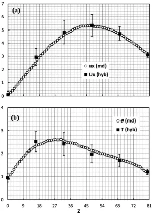
Fig. 6shows the comparisons between MD and hybrid results
for velocity (Fig. 6(a)) and temperature (Fig. 6(b)). The agreement between the hybrid results and the pure MD simulation is very good both for temperature and streaming velocity. In both cases, the error bars of the hybrid data are relatively high, but acceptable. This depends on the fact that the MD part of the algorithm intro-duces fluctuations in the results. Numerical noise exists also in the pure MD simulation, but the total number of atoms is higher and, therefore, fluctuations are smaller. Error bars for the full MD data are not reported, but they are considerably smaller than the hybrid ones. More details on the fluctuations (and how to reduce them) are given below.
Other issues that deserve attention are the velocity and temper-ature discontinuities at the boundaries. Stochastic walls do not generate slip asFig. 6(a) shows. They do, however, produce a tem-perature jump. In this specific case, for instance, we imposed T1w¼1 andT
2
w¼1:5 at the walls but, asFig. 6(b) indicates, the
tem-perature in the bin closest to each wall is slightly lower (respec-tively 0.9 and 1.2). InFig. 6, the effect of the temperature jumps is rapidly dominated by the presence of viscous dissipation but, without this dissipation, they would involve a larger portion of the fluid, as discussed in the next section.
6.2. Wall correction
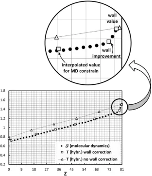
In the previous example, the effect of the temperature jump at the walls is limited to the first bin near the wall. There are situa-tions, however, where more bins are necessary. InFig. 7, for in-stance, the temperature profile between two walls at different temperatures (T1
W¼1 andT 2
W¼2 is reported. All the other
simula-tion condisimula-tions (for both hybrid and full-MD cases) are the same as
inFig. 6, but here there are no body-forces (g= 0) and neither wall
moves (U1 W¼U
2
W¼0); the fluid, therefore, is at rest and heat is
only transferred by conduction. Basically, we have here the classic one–dimensional heat equation at steady state, whose analytical (macroscopic) solution is simply a straight line connecting the wall temperatures. With the exception of the wall regions, the full MD solution confirms this linear behaviour (seeFig. 7). In this case, however, the temperature jumps at the walls are not strictly lim-ited to the solid–fluid interface as inFig. 6, but involve a region of approximately two molecular lengths. The imposed temperature at the walls isT1W¼1 andT
2
W¼2; in the first bin next to the walls,
[image:8.595.135.449.375.739.2]it drops to respectively 0.8 and 1.6. But, unlike the previous case, the temperature keeps falling and in the second closest bin it goes approximately to 0.7 and 1.3 respectively. When we calculate the hybrid solution, if we simply use the method described in Section4 (in which only the first bin closest to the walls is considered), we obtain the first profile (triangular markers) inFig. 7. The calcula-tion of only one value of the temperature in the bin nearest to the wall is therefore not enough and does not guarantee, in this
case, a correct temperature profile. To correct this problem, we also consider a second temperature point at the wall (the second near-est bin referred as ‘wall improvement’ inFig. 7). By using this sim-ple method, the hybrid solution improves considerably, asFig. 7 (square markers) indicates. InFig. 7, we only report the average re-sults. Since the two hybrid profiles are close to each other, the error bars would makeFig. 7difficult to read. The fluctuations, however, are of the same relative magnitude as inFig. 6.
6.3. Viscous dissipation
The velocity profile inFig. 6(a) is not parabolic because part of the energy necessary to maintain the velocity gradient degrades to heat through viscous dissipation. As a consequence, the temper-ature and, therefore, the viscosity are not constant. The same phe-nomenon can be observed, at the nanoscale, also in the case of Couette flow.Fig. 8reports the case where no gravity-like force is considered; the two walls have different velocities (U1
W¼0
and U2W¼4) but the same temperature (T 1 W¼T
2
W¼1). The
remaining simulation conditions (for both hybrid and full-MD cases) are the same as inFig. 6with the difference that, here, the MD simulations of the hybrid model are run for 60,000 time steps instead of 6000. This does not mean that the calculation of the Cou-ette flow requires a higher accuracy than the cases previously
investigated. We simply want to show, as discussed below, that increasing the statistical accuracy of the single MD steps reduces the overall fluctuations of the hybrid method.
The results are illustrated inFig. 8. The analytical (macroscopic) solution of the Couette flow problem would be a straight line con-necting the two wall velocities. Since in the case of stochastic walls the wall-slip is small, we do not have, for the velocity, the issue of the wall correction as for the temperature (see Section 6.2). The full-MD results, however, do not show a perfectly linear behaviour
(Fig. 8(a)). This is due to the viscous dissipation, which heats the
fluid and raises the temperature (Fig. 8(b)). In a macroscopic chan-nel, the amount of heat generated in this way would be negligible, but in a nano-channel the situation is different. Since the fluid is not isothermal, the viscosity in the channel is not constant so the velocity profile is not perfectly linear. This is particularly true near the walls where the temperature gradients are higher. The hybrid results again match very well the full-MD data, confirming the effectiveness of our method.
InFig. 8, we report, as inFig. 6, the temperature and velocity
[image:9.595.160.448.346.739.2]values at the nodes (black markers). In this case, however, we also show the values in the constrained region (grey markers) of the ‘layered’ cell. This gives an idea of the relative size of the MD cells used in the hybrid model. InFig. 8, the wall improvement (see Sec-tion6.2) is used only for the temperature profile (the two darker
grey and slightly smaller markers near the walls inFig. 8(b)). For the velocity (Fig. 8(b)), no wall improvement is necessary because, as already mentioned, stochastic walls do not produce slip for liquid flows.
The error bars inFig. 8are considerably smaller than those in
Fig. 6. This is due to the fact that, in this case, the MD simulations
of the hybrid algorithm are run for 60,000 time steps instead of 6000. This implies higher accuracy of the microscopic solver and, consequently, smaller overall fluctuations in the hybrid solution. The price to pay for this improvement is, of course, a greater
com-putational time: a trade-off between accuracy and comcom-putational time is, as usual, required.
6.4. Isothermal case
Up to now, we have considered non-isothermal cases, but we can also test the accuracy of our method for isothermal flows, which require only the momentum equation to be solved.Fig. 9
shows the MD results for a 5575 unit cells box
[image:10.595.96.489.201.444.2](5.45.481 reduced units), with density
q
= 0.8 and [image:10.595.90.502.481.738.2]Fig. 9.Comparisons between full MD and hybrid velocity profiles for isothermal Poiseuille flow.
gx= 0.0075; the velocity of both (stochastic) walls isU1w;2¼0 and
the temperature isT1;2
w ¼1. The domain in thez-direction is
di-vided into 150 bins. We run two simulations for 250,000 time steps (Dt= 0.005). In the first one, no temperature control is imple-mented and the temperature rises slightly (T1.5 in the centre of the channel). In the second one the dissipation heat is removed with a velocity rescaling (T= 1) every 10,000 time steps so that the average temperature remains approximately constant in the chan-nel. The streaming velocity is not particularly affected by the
tem-perature control. Fig. 9 shows the velocity profile for the
controlled case, but the profile for the temperature-non-controlled case is very similar. Concerning the hybrid results, we run the simulation under the same conditions of Fig. 6, but gx= 0.0075,Uw= 0 on both walls,Lz= 81 andN= 5. The fluid
tem-perature in the constrained regions of every node is fixed to T= 1. Once the temperature is controlled in the ‘frames’, and since the MD boxes used in the hybrid scheme are small, the tempera-ture does not rise particularly and no further temperatempera-ture control is necessary. While forFigs. 6–8a relaxation factor (see Eq.(28))
a
= 0.5 was used, here no relaxation (a
= 0) is employed.Fig. 9shows the comparison between our hybrid results and the
parabolic profile. As already discussed, the hybrid results are rather noisy and this can be seen from the error bars. While forFig. 8we used more MD time steps than forFig. 6to show how this de-creases the fluctuations, here we did not use a relaxation factor
in order to show how this increases the fluctuations. Despite the higher noise, however, the algorithm remains stable and the aver-ages inFig. 9closely follow the MD profile.
6.5. Macroscopic validation
So far, we validate our method by comparing hybrid and full-MD results. This is, as already mentioned, common practice and, up to now, we conformed to it. In general, however, this type of validation is restrictive because, in this way, we only test the mod-el for small systems, despite the fact that the reason why we study hybrid algorithms in the first place is to be able to simulate sys-tems much larger than MD is capable of simulating within reason-able computational times. Moreover, in order to show a visually more effective comparison with the MD results, we used more nodes than necessary in our previous hybrid simulations. Thefore, the computational speed-up of the hybrid algorithm with re-spect to MD cannot be always fully appreciated from these particular examples.
[image:11.595.154.454.354.523.2]Normally, there is not much of a choice since we are restricted by the relatively limited size of the full-MD suitable cases. An iso-thermal Lennard–Jones fluid in a large channel, however, can be considered, with a certain approximation, Newtonian if the strain-rate does not vary excessively in the domain. We can, there-fore, take advantage of this circumstance and compare our results
[image:11.595.125.476.564.739.2]Fig. 11.Fitting improvement by using the continuum estimation.
with the corresponding parabolic profile in order to assess the accuracy of the hybrid model for larger channels. Here, we simu-lated an isothermal channel (T= 1, N= 11, U1;2
w ¼0, gx= 105,
a
= 0.1 and 101010 unit cells per node; other conditions are the same as inFig. 8) of sizeLz= 3000 reduced units. If we considerthat in many practical cases the
r
parameter of the Lennard–Jones potential is between 3 and 6 Å, this means that we are now simu-lating a channel with a width between 1 and 2l
m. The hybrid cal-culation took only a few hours on a simple Desktop computer (Intel i-7-26000 QuadCore 3.4 GHz, 8 GB RAM), but it would be consider-ably harder to run a full MD simulation. We cannot even quantify how large is the speed-up gain in this case because for MD it would be impossible to simulate a channel of this size without the aid of a supercomputer.Fig. 10shows, as expected, the clear parabolic profile of the
hy-brid data. If, from the fitting parabola, we determine the viscosity, we find a value of 1.9 reduced units, which is perfectly consistent with the non-equilibrium equation of state for Lennard–Jones flu-ids[2]. The fluctuations are here kept under control by using longer MD steps, as inFig. 8, and a lower relaxation value of 0.1. InFig. 10 only the values at the constrained regions are reported. In this case, the MD cells have the same length of the previous examples, but, since here the overall size of the channel is much larger, they look considerably smaller. Moreover, we employed in this case a smal-ler number of nodes relative to the size of the macroscopic domain. In general, the larger the system the more efficient is the hybrid computation because the optimal ratio betweenNand the size of the macroscopic domain decreases.
We should not be misled by the apparent simplicity of this example. The parabolic profile is naturally recreated by the hybrid solver without anya prioriassumption on the stress. The fact that from the intrinsic complexity of the intermolecular interactions we arrived, as expected in this particular situation, to the relatively simple Newton law of viscosity is a significant result and a good test for our method.
7. Conclusions
We have proposed a new algorithm within the HMM/PWC framework, which is based on the calculation of the velocity/tem-perature Laplacians at internal nodes and the velocity/temvelocity/tem-perature values at boundaries. The algorithm performed very well in all test cases considered. Since our hybrid method needs the estimation of second derivatives from MD profiles, a certain level of fluctuation in the result is expected. We discussed which factors affect the fluctuations and how they can be dramatically reduced by using higher relaxation factors and longer MD steps. A third way of reducing the fluctuations is discussed inAppendix B.
There are three main advantages in our method. Two have al-ready been mentioned: the algorithm works for non-isothermal flows and it does not need the calculation of the Irving–Kirkwood fluxes. The third advantage is that direct knowledge of the source terms (gin Eq.(7)and
s
:$Uin Eq.(8)is not required since their effect is automatically included in K and N (see Eqs. (13) and (14)). At first sight, the importance of this fact can be underesti-mated. The value of the gravity-like term g, for instance, should be perfectly known so its calculation does not seem to be an issue. In practical microfluidic applications, however, the flow is not usu-ally generated by simple gravity-like forces as in Eq.(7). More of-ten, the driving force comes from electro-osmotic, piezoelectric, or magnetic effects[1,17]. While it is possible to implement these in an MD simulation, their effect on the continuum model cannot be concentrated in a simple constant asgin Eq.(7). This makes our method viable also when these forces are not perfectly known at the macroscopic level, and this is clearly an advantage in some practical situations. For the non-isothermal case, the benefit iseven more obvious since the
s
:$Uterm is more complex thang. The calculation of the relatively complicated viscous dissipative term (enclosed ins
:$U) is, in our model, not required, but emerges automatically from the Laplacian.There are, moreover, some features of the algorithm that make it attractive from a practical point of view. Both the discrete and the continuous parts require minimal changes from, respectively, standard MD codes and partial differential equations (PDE) numer-ical solvers. Concerning the atomistic model, for instance, since ri-gid periodic boxes are employed, the only real modification with respect to a standard MD code is the presence of the constrain re-gion. Concerning the continuum solver, once the molecular source term is introduced into Eqs.(21) and (22), we simply obtain the Poisson equation, which is one of the most studied PDEs, and many numerical solvers are available for its solution.
The main purpose of this article is to introduce, for the first time, the Laplacian method and, for this reason, the issue of the algorithm numerical efficiency is not directly addressed here. There are at least three possible lines of improvement (namely, the assessment of the minimal number of nodes for a given accu-racy, the introduction of a ‘‘seamless’’ strategy as proposed by E et al.[15], and a more robust estimation of the Laplacian), but they are left for future work. Despite this, Section6.5provides an idea of the huge computational savings that are expected in large geome-tries by using the Laplacian method instead of the full MD.
Acknowledgments
This research is financially supported by EPSRC Programme Grant EP/I011927/1.
Appendix A. Reduced units
In our simulations, we use the Lennard–Jones potentials
VLJij ¼4
r
LJ rij 12r
LJ rij 6 " #; ðA:1Þ
where
is the characteristic energy level of the potential,r
LJthemolecular length scale andrijthe distance between atomsiandj.
In this case, the most appropriate system of units adopts
r
LJ,m(the mass of the molecule) and
as units of length, mass and en-ergy, respectively. All other variables are determined in relation to these e.g.r¼ r
r
LJ ðlengthÞ; ðA:2Þ
t¼ ffiffiffiffiffiffiffiffiffiffiffiffiffiffiffiffit
=mr
2LJ
q ðtimeÞ; ðA:3Þ
u¼u
ffiffiffiffiffi m
r
ðvelocityÞ; ðA:4Þ
T ¼TkB
ðtemperatureÞ; ðA:5Þf¼f
r
LJ ðforceÞ; ðA:6ÞP¼P
r
3
LJ
ðpressureÞ; ðA:7Þq
¼q
r
3
LJ
l
¼l
r
3
LJ ffiffiffiffiffiffiffi m
p ðviscosityÞ; ðA:9Þ
g¼gm
r
LJ ðaccelerationÞ; ðA:10Þwhere each dimensional unit has a corresponding (asterisked) re-duced unit, which is dimensionless. In order to simplify the nota-tion, the asterisk is not used in this article; nonetheless all the numerical values are always reported in reduced units.
Appendix B. Continuum estimation for noise reduction
The calculation of the Laplacian is central in our method and, at the same time, the main source of noise. In this article, we used two ways of reducing the fluctuations: longer MD steps and the relaxation factor. We saw that the price to pay for using these methods consists in longer computational times. There is, however, a third idea, which does not have this drawback, but, on the other hand, requires an initial approximation of the solution. In the val-idation cases discussed in this study (Section6), we did not use this third approach because we wanted to test our method in the worst possible scenario, where no approximation is available. In general, however, this can be obtained by calculating the continuum solu-tion. With ‘‘continuum solution’’ in this case, we do not mean the solution calculated during the macroscopic step of the hybrid algo-rithm, but the solution we would obtain by solving only the mac-roscopic equations without any micmac-roscopic refinement. We could, for instance, close Eqs.(7) and (8)with, respectively, Newton’s law of viscosity and Fourier’s law of heat conduction and look for a rea-sonable estimation of the viscosity and the thermal conductivity.
A practical example can help us explaining this method. We take into consideration a framed computational cell composed of 101012 unit cells. The streaming velocity and temperature are constrained in the 2nd and 11th bin in the z direction to, respectively,U1= 0 andT1= 1, andU2= 0.1 andT2= 1. The acceler-ationgxis fixed to 0.01, while the remaining parameters are the
same ofFig. 5. While the simulation progresses, we sample every 50 time steps the molecular velocities. When a certain numbern of samples is accumulated (we choosen= 5, 10, 20, 50, 100, 250, 500, 1000 and 100,000), we calculate the average streaming veloc-ity in each bin. The white circles inFig. 11, for instance, represents the velocity values atn= 50; they are significantly scattered be-cause they are based on a small number of samples. Asnincreases, the velocity profile becomes more accurate. The profile labelled with ‘‘n1’’ (black diamonds) represents the velocity calculated with a very high number of samples (n= 100,000). Since in this case a high number of samples are used, the data follow a well-de-fined curve as indicated inFig. 11. If we increasenbeyond this va-lue, no noticeable effect on the velocities is observed and this is the reason why we named this profilen1.
These velocity values (white circles inFig. 11) are then fitted to a parabola whose curvature, as already discussed in Section5, is sent to Eq.(27). InFig. 11, the parabola in question is the one la-belled with ‘‘no continuum estimation’’. The higher n, the more accurate is the curvature. The white squares inFig. 12show how the curvature varies withn. Low values ofnsignify faster MD steps, but, at the same time, lower accuracy and, therefore, higher noise. We now introduce an estimate of the solution. We may, for in-stance, assume that the fluid is Newtonian with
l
= 2. We may also know that the accuracy of this estimation is ±50% and, therefore, the real solution is bounded by the continuum profiles calculated withl
= 1 andl
= 3 as indicated inFig. 11. Previously, the parabola labelled with ‘‘no continuum estimation’’ was calculated by stan-dard unweighted fitting, now we can use the approximate solution and achieve a weighted fitting. Maximum weight (w= 1) is given tothe data in the grey area ofFig. 11. The weight of the white circles outside this zone is reduced proportionally to the square of their distance from the grey area. Other strategies are possible, but the logic is always the same: the farther the circle is from the maxi-mum confidence zone, the smaller the weight should be. If we re-peat the fitting with these weights, we obtain the parabola labelled ‘‘with continuum estimation’’, which is considerable closer ton1 than the ‘‘no continuum estimation’’ one. The triangles inFig. 12 show that the curvatures calculated with the continuum estima-tion are, at lown, considerably more accurate than the ones calcu-lated without continuum estimation. Higher confidences in the continuum approximation produce higher accuracies in the curva-ture, as the
l
= 2 ± 25% curve inFig. 12(the maximum confidence zone is now delimited by thel
= 1.5 andl
= 2.5 curves) indicates. The method described here can be useful to further reduce the fluctuations. We must keep in mind, however, that it requires, at each macro-step, the calculation of two continuum solutions: one for the upper limit and the other for the lower limit of the maximum confidence zone. This, nevertheless, should not be a problem in practice for two reasons. First, we do not seek the con-tinuum solution in the whole macroscopic domain, but only in the zones covered by the MD solver. Second, it is true that the compu-tation of the continuum solution requires additional computa-tional time, but usually the bottleneck of the hybrid approach lays in the microscopic rather than the macroscopic step. There-fore, if we could reduce the fluctuations by employing the macro-scopic rather than the micromacro-scopic solver, we would, in general, save time.References
[1]P. Abgrall, N.T. Nguyen, Nanofluidics, Artech House Publishers, 2009. [2]A. Ahmed, R. Sadus, Nonequilibrium equation of state for Lennard–Jones fluids
and the calculation of strain-rate dependent shear viscosity, AIChE J. 57 (2011) 250–258.
[3]A. Alexiadis, S. Kassinos, Molecular simulation of water in carbon nanotubes, Chem. Rev. 108 (2008) 5014–5034.
[4]A. Alexiadis, S. Kassinos, Self-diffusivity, hydrogen bonding and density of different water models in carbon nanotubes, Mol. Simul. 34 (2008) 671–678. [5]A. Alexiadis, S. Kassinos, Influence of water model and nanotube rigidity on the
density of water in carbon nanotubes, Chem. Eng. Sci. 63 (2008) 2793–2797. [6]A. Alexiadis, S. Kassinos, The density of water in carbon nanotubes, Chem. Eng.
Sci. 63 (2008) 2047–2056.
[7]F. Alfieri, M.K. Tiwari, I. Zinovik, D. Poulikakos, T. Brunschwiler, B. Michel, 3D integrated water cooling of a composite multilayer stack of chips, J. Heat Transfer 132 (2010) 21402–21409.
[8]M. Allen, D. Tildesley, Computer Simulation of Liquids, Clarendon Press, Oxford, 1987.
[9]H. Akima, A new method of interpolation and smooth curve fitting based on local procedures, J. ACM 17 (1970) 589–602.
[10] N. Asproulis, M. Kalweit, D. Drikakis, A hybrid molecular continuum method using point wise coupling, Adv. Eng. Softw. 46 (2012) 85–92.
[11]D. Drikakis, N. Asproulis, Multi-scale computational modelling of flow and heat transfer, Int. J. Numer. Meth. Heat Fluid Flow 20 (2010) 517–528. [12]R.B. Bird, W.E. Stewart, E.N. Lightfoot, Transport Phenomena, second ed., John
Wiley & Sons, 2007.
[13]M.K. Borg, D.A. Lockerby, J.M. Reese, A multiscale method for micro/nano flows of high aspect ratio, J. Comput. Phys. 233 (2013) 400–413.
[14]J. Cormier, J.M. Rickman, T.J. Delph, Stress calculation in atomistic simulations of perfect and imperfect solids, J. Appl. Phys. 89 (2001) 99–104.
[15]W. E, W.C. Ren, E.C. Vanden-Eijnden, A general strategy for designing seamless multiscale methods, J. Comput. Phys. 228 (2009) 5437–5453.
[16]N.G. Hadjiconstantinou, A.T. Patera, Heterogeneous atomistic-continuum representations for dense fluid systems, Int. J. Mod. Phys. C 8 (1997) 967–976. [17]G. Hu, D. Li, Multiscale phenomena in microfluidics and nanofluidics, Chem.
Eng. Sci. 62 (2007) 3443–3454.
[18]J.H. Irving, J.G. Kirkwood, The statistical mechanical theory of transport processes. IV. The equations of hydrodynamics, J. Chem. Phys. 18 (1950) 817– 829.
[19]M. Gad-El-Hak, MEMS: Introduction and Fundamentals, Taylor & Francis, 2006.
[20] I.G. Kevrekidis, G. Samaey, Equation-free multiscale computation: algorithms and applications, Annu. Rev. Phys. Chem. 60 (2009) 321–344.
[21]J. Koo, C. Kleinstreuer, Viscous dissipation effects in microtubes and microchannels, Int. J. Heat Mass Transfer 47 (2004) 3159–3169.
[23]T. Li, Y.G. Lv, J. Liu, Y.X. Zhou, A powerful way of cooling computer chip using liquid metal with low melting point as the cooling fluid, Forsch. Ingenierwes. 70 (2005) 243–251.
[24]J. Liu, S. Chen, X. Nie, M.O. Robbins, A continuum-atomistic simulation of heat transfer in micro- and nano-flows, J. Comput. Phys. 227 (2007) 279– 291.
[25]T.W. Lion, R.J. Allen, Computing the local pressure in molecular dynamics simulations, J. Phys.: Condens. Matter 24 (2012) 284133.
[26]J.F. Lutsko, Stress and elastic constants in anisotropic solids: molecular dynamics techniques, J. Appl. Phys. 64 (1988) 1152–1154.
[27]K.M. Mohamed, A.A. Mohamad, A review of the development of hybrid atomistic-continuum methods for dense fluids, Microfluid. Nanofluid. 8 (2010) 283–302.
[28]W.D. Nicholls, M.K. Borg, D.A. Lockerby, J.M. Reese, Water transport through (7, 7) carbon nanotubes of different lengths using molecular dynamics, Microfluid. Nanofluid. 12 (2012) 257–264.
[29]W.D. Nicholls, M.K. Borg, D.A. Lockerby, J.M. Reese, Water transport through carbon nanotubes with defects, Mol. Simul. 38 (2012) 781–785.
[30]D.C. Rapaport, The Art of Molecular Dynamics Simulation, second ed., Cambridge University Press, 2004.
[31]W. Ren, W. E, Heterogeneous multiscale method for the modeling of complex fluids and micro-fluidics, J. Comput. Phys. 204 (2005) 1–26.
[32]B.D. Todd, D.J. Evans, P.J. Daivis, Pressure tensor for inhomogeneous fluids, Phys. Rev. E 52 (1995) 1627–1638.