Optimal dynamic operations scheduling for small-scale satellites

IAC-12-B4.3.7

OPTIMAL DYNAMIC OPERATIONS SCHEDULING FOR SMALL-SCALE SATELLITES

Eirini Komninou

University of Strathclyde, Glasgow, United Kingdom

[email protected]

Massimiliano Vasile

University of Strathclyde, Glasgow, United Kingdom

[email protected]

Edmondo Minisci

University of Strathclyde, Glasgow, United Kingdom [email protected]

Abstract A satellite’s operations schedule is crafted based on each subsystem/payload operational needs, while taking into account the available resources on-board. A number of operating modes are carefully de-signed, each one with a different operations plan that can serve emergency cases, reduced functionality cases, the nominal case, the end of mission case and so on. During the mission span, should any operations planning amendments arise, a new schedule needs to be manually developed and uplinked to the satellite during a communications’ window. The current operations planning techniques offer a reduced number of solutions while approaching operations scheduling in a rigid manner. Given the complexity of a satellite as a system as well as the numerous restrictions and uncertainties imposed by both environmental and technical parameters, optimising the operations scheduling in an automated fashion can offer a flexible approach while enhancing the mission robustness. In this paper we present Opt-OS (Optimised Operations Scheduler), a tool loosely based on the Ant Colony System algorithm, which can solve the Dynamic Oper-ations Scheduling Problem (DOSP). The DOSP is treated as a single-objective multiple constraint discrete optimisation problem, where the objective is to maximise the useful operation time per subsystem onboard while respecting a set of constraints such as the feasible operation timeslot per payload or maintaining the power consumption below a specific threshold. Given basic mission inputs such as the Keplerian elements of the satellite’s orbit, its launch date as well as the individual subsystems’ power consumption and use-ful operation periods, Opt-OS outputs the optimal ON/OFF state per subsystem per orbital time step, keeping each subsystem’s useful operation time to a maximum while ensuring that constraints such as the power availability threshold are never violated. Opt-OS can provide the flexibility needed for designing an optimal operations schedule on the spot throughout any mission phase as well as the ability to auto-matically schedule operations in case of emergency. Furthermore, Opt-OS can be used in conjunction with multi-objective optimisation tools for performing full system optimisation. Based on the optimal operations schedule, subsystem design parameters are being optimised in order to achieve the maximal usage of the satellite while keeping its mass minimal.

Keywords – Optimal operations scheduling, Optimal satellite design, Ant Colony Optimisa-tion, Multi-objective optimisaOptimisa-tion, Maximal Satellite Usage.

NOMENCLATURE

ρ/ξ Global/Local Pheromone evaporation constant τ0 Initial pheromone level

τij Pheromone edge between node i and j

C Mean power consumption throughout mission α Pheromone parameter weight

q0 Exploration parameter

q Randomly generated real number

pij Probability of moving from node i to node j

k Ant index with k = 1,2...m m Number of ants per colony

n Number of timesteps of mission timeline r Number of revolutions

S Number of subsystems onboard OPmax Maximum useful operation period

Jik Candidate list of nodei, antk

Q+ _{Best-so-far quality}

Imax Definite optimisation termination criterion

a Semimajor axis e Eccentricity i Inclination

RAAN Right Ascension of the Ascending Node ω Argument of periapsis

1 INTRODUCTION

Designing satellite operation plans is a strenuous task, deriving from the cooperative work of several disciplines. After examining the mission concept and supporting architecture, a preliminary mission plan is developed based on the mission objectives. According to the mission payloads and subsystems on-board, operation requirements are formed based on operation timing per payload or subsystem, link budgets, data budgets and so on.

Depending on the mission phase and information available, the operations plan is initially formed and then being updated whenever new information is arising. Occasionally information is not available since the operations design isn’t very far along or not specified yet, thus leading to assumptions. When more information becomes available, the cost of changes can be determined by modifying the operations concept and re-evaluating the cost and complexity of the mission. Examples of ob-jectives and constraints shaping mission operations planning are: Maximisation of real-time contact and commanding versus on-board autonomy and data-storage, maximisation of the involvement of educational institutions using amateur university-run ground stations for instance, limiting the image budget to a specific number of images, using a specific tracking network, limiting the mission cost etc.

Based on the launch dates/windows, trajectory profile, mission phases and the activities required during each phase, a final set of observation and operation strategies is devised, based on the mis-sion description and constraints. While operation strategies derive from mission objectives, sometimes they highly depend on the designer’s background or experience. Therefore, an identification of whether the strategies used are mandatory, highly desirable or based on personal and organisational preferences, needs to be performed throughout the mission operations planning process.

Apart from nominal operations, designers need to take into account various mission scenarios corresponding to reduced functionality operations (e.g post-launch activation phase), emergency operations (e.g instrumentation malfunction) etc. Such scenarios can be tackled by designing a specific set of operational modes, developed to minimise the probability of mission failure by performing a set of predefined actions aiming at isolating and solving possible errors that can occur. Each mode contains a different set of actions based on its functionality, for example a safe mode is designed in order to tackle

a potential malfunction. For instance if the power availability is greatly decreased due to an electrical malfunction, all non-vital subsystems including payloads are turned off in order to save energy and avoid a power surge while the telecommunications are reduced to an absolute minimum.

Based on the aforementioned facts, it is clear that mission operations planning is not only a challenging and time consuming task, but can also be rigid and prone to errors. More than 43% of failures may be attributed to human error [1, 2, 3, 4], therefore enhancing the robustness of mission design is of uttermost importance. The proposed work aims at tackling these issues by offering tools and methodologies for dynamically performing optimal operations scheduling on the spot while maximising the satellite usage.

Furthermore, an integrated system-operation ap-proach is presented, aiming at designing a full optimal satellite system. Using a multi-objective agent based optimiser [5], a Pareto set of points is formed corresponding to optimal satellite designs, with each Pareto point representing a low lying optimiser. Every point included in the Pareto set represents a vector of values corresponding to optimal design parameters per subsystem on-board the satellite leading to an optimal system design. The aforementioned integrated approach can lead to robust system designs developed in a timely manner and at a lower cost, thus making space accessible to a wider spectrum of institutions with lower budgets.

2 DYNAMIC OPERATIONS

SCHEDULING

Operations scheduling can be a highly dynamic pro-cess. Depending on the mission phase and complex-ity, the satellite’s health and other factors that can affect the progress of the mission, new operations schedules need to be designed on a tight time-frame in order to ensure the mission success.

elements comprising the mission, based on the mis-sion requirements and constraints. Once all elements have been established, they are passed to an Ant Colony System based optimiser in search of the op-timal operations schedule based on the requirements and constraints set. The final result is an optimal operations schedule developed in an automated man-ner, on the spot.

The following sections aim at giving a background of the Ant Colony System structure and operation, fol-lowed by a more detailed view of the proposed tools and methodologiesl for performing optimal dynamic operations scheduling.

2.1 Ant Colony System

The Ant Colony System (ACS) [6, 7, 8, 9, 10] was developed by Dorigo and Gambardella as an evolu-tion of the first agent based algorithm based on ants’ behaviour, namely the Ant System (AS), able to solve complicated combinatorial optimisation prob-lems more efficiently. It was first used for solving NP-hard problems, like the Traveling Salesman Problem (TSP) [11] where the shortest Eucledian distance path needs to be found among a set of cities to be visited.

All ant-based algorithms utilise a common basic idea. Ant colonies explore the search space in a pseudo-random manner, searching for possible routes from the ant nest (starting point) to the food source (end-ing point) with the aid of a ’compass’ (heuristic infor-mation), aiming at finding the shortest path possible between the start and end. Ants exchange informa-tion with each other via the means of pheromone deposition, a chemical used in real life ant colonies for leading ants towards good solutions [12]. The process is iterative, aiming at finding the best solu-tion possible throughout each iterasolu-tion and sharing that experience throughout the next iterations. At the end of each iteration, ants deposit pheromone throughout the best-so-far path as a means of syn-ergy thus communicating their experience to the rest of the agents. This enhances the pheromone level at this path, thus making it more attractive for the ants to follow. Since pheromone is time dependent, it evaporates with time, therefore paths which do not receive pheromone enhancement become less attrac-tive for the agents to follow. The ACS incrementally forms paths while searching for the optimal solution, using the steps described in Algorithm1.

First, the basic algorithm parameters are ini-tialised. A uniform layer of pheromone is laid on the search space in order to keep the probability dis-tribution deriving from Eq. (3) positive. Lack of initial pheromone would lead to a probability

dis-Algorithm 1ACS algorithm Definem, Ilast, τ0, q0, α, β

Form candidate listJi ∀i∈[search space] whileImaxnot met do

Place all agents on start fork = 1:mdo

whilenot terminatedo Calculateηij

Decide nextjk _{using Eq. (2)}

Perform local pheromone update on edgeij using Eq. (4)

end while end for

Calculate the quality of all toursTk FindT+

Perform global pheromone update onT+ using Eq. (5)

end while

tribution of zeros, thus halting the ants and pre-venting them from exploring the search space. The ants (also known as agents) start exploring the search space in a pseudo-random fashion (their exploration is biased by the existence of pheromone in combina-tion with one or multiple heuristics i.e values acting as a compass), incrementally constructing possible optimal routes. Once all agents of a single colony complete a full tour from the starting to the end-ing point, routes’ lengths are measured, the short-est route, T+_{, is enhanced with pheromone and all}

agents are placed back to the starting point in order to proceed to the next round of exploration. This it-erative process continues until the optimisation ter-mination criterion,Imax, is met. A step by step

ex-planation of Algorithm1 can be found below. - Define the number of agents ,m, per colony,

optimisation termination criterion ,Ilast,

explo-ration vs exploitation parameter ,q0, pheromone

parameter weight ,α, heuristic parameter weight ,β. The initial pheromone level of the search space ,τ0, is calculated as follows

τ0(t) = (n·Lnn)−1 (1)

with Lnn being the length of the nearest

neighbour tour, performed using the nearest-neighbour classification algorithm [13] ,n the total number of nodes included in the search space.

- Construct the candidate list of every node in the search space ,Ji, withi∈[search space]. In

on nodes included in a candidate list i.e a set of nodes Jk

i in the vicinity of nodei where ant k

is situated at. Unvisited nodes contained in the candidate list are examined first, having priority over the rest of the nodes contained in the search space.

- While the optimisation termination criterion ,Imax, is not met

- Place all ants on the starting node. - For all the ants ,m, comprising a colony - While the ants have not yet reached the ending

node

- Calculate the length heuristic for edge ij ,ηij =

L−_ij1, withLij being the euclidean length of edge

ij.

- Choose the next ant step ,j, on the basis of the

pseudo-random proportional rule. The transi-tion of ant k, situated on node i, to node j, is decided according to Eq. (2)

j=

(

arg max_u∈Jk i {[τiu(t)]

α_[ηiu]β_{} ifq≤q}

0

J ifq > q0

(2)

where q is a randomly generated real number uniformly distributed over [0,1],q0is a tunable

parameter in the interval (0,1),J ∈Jk

i selected

according to the transition probability distribu-tion below

pkij(t) =

[τij]α·[ηij]β

P

l∈Jk i[τil]

α_·[η il]β

(3)

where τij is the pheromone level of edge ij, α

andβare weight parameters. Likewise,τilis the

pheromone level of edgeilandηilis the heuristic

value of edgeilwith l being every node compris-ingJ_ik. Tuningq0 enhances the exploitation vs

exploration option, where q ≤ q0 aims in

ex-ploiting the available knowledge whereasq > q0

aims at exploring the available search space. - Perform local pheromone update on edge ij.

While exploring the search space, ants perform a local pheromone update after each step. Once antktakes a step from nodeito nodej, it up-dates the pheromone level of edge ij according to Eq. (4).

τij(t)←(1−ξ)·τij(t) +ξ·τ0(t) (4)

whereτij is the pheromone level of edgeij,ξ is

the local pheromone evaporation rate parame-ter,τ0 is the initial pheromone trail value.

The local pheromone update aims at subtract-ing a small fraction of the pheromone on the edge that ant k just visited. That way, edge ij becomes less attractive to the ants to follow, thus enhancing exploration. By shuffling ants’ paths with the use of the local pheromone up-date, the probability of finding better solutions and avoiding stagnation is increased.

- End the while condition - End the for loop.

- Calculate the quality of each ant’s tour ,Tk_{, on}

the basis of euclidean distance.

- Find the best-so-far tour ,T+_{, corresponding to}

the shortest length tour.

- Perform a global pheromone update on the edges comprising the best-so-far tour ,T+, ac-cording to theglobal pheromone update rule

τij(t)←(1−ρ)·τij(t) +ρ·∆τij(t) (5)

where ij are the edges comprising T+_{, ρis the}

pheromone evaporation rate parameter and ∆τ ij(t) = (L+₎−1

with L+ _{being the length of T}+ _{The global} pheromone update allows colony members to spread all acquired experience among them, pro-moting synergy between ants thus leading to a faster convergence towards the optimal solution. - End the while condition.

The following section describes how the ACS phi-losophy is utilised in order to achieve optimal mis-sion operations scheduling, showing that Ant Colony Optimisation algorithms can be applied to solving all types of problems, physical or conceptual ones. 2.2 Optimal Operations scheduler (Opt-OS)

Opt-OS is a tool designed for deriving the optimal mission operations schedule automatically, based on the mission requirements and available resources. The objective is to maximise the satellite usage by maximising the useful operation period per subsys-tem while respecting a set of constraints such as the feasible operation timeslot per payload or maintain-ing the maximum power consumption below a spe-cific threshold.

First, the orbit is being designed based on its classi-cal orbital elements [14]. Based on the orbit, an ini-tial operations plan,OPmax, is derived,

correspond-ing to the maximum useful operation time period allocation per subsystem on-board.

The satellite is modeled using a set of analytical models able to estimate the physical and electrical characteristics per subsystem, based on a specific set of design and environmental inputs. Utilising the physical and electrical characteristics per subsys-tem as well as theOPmax, a search space is created

corresponding to all the possible states that could be applied in order to derive an operations sched-ule. A nature-inspired metaheuristic, namely an Ant Colony System inspired algorithm, is then used for exploring the search space in search of the optimal operations schedule. The aforementioned process of-fers design flexibility and enhanced robustness as it allows the designer to derive an optimal operations schedule on the spot, respecting the constraints set such as the power availability, target visibility and so on. Furthermore, Opt-OS can be used in case of emergency or partial failure (e.g partial instrument or subsystem failure imposing unscheduled changes in the operations plan).

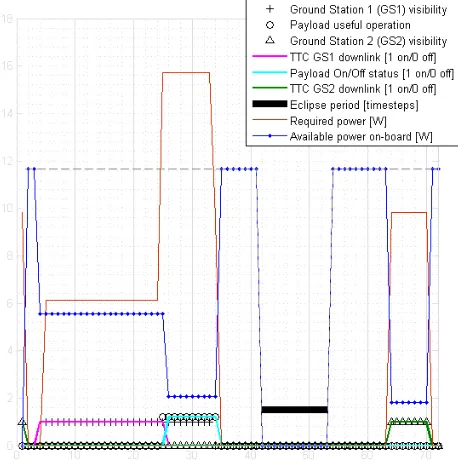
Figure 1: Optimal operations plan. Note that there is no available power during eclipse time (battery malfunction). Also, the generated power during daylight is limited.

Figure 1 shows an example of how Opt-OS can schedule operations on the spot based on the

avail-able resources on-board. In this instance the satel-lite’s batteries cannot be charged due to a malfunc-tion. Furthermore, the solar arrays are not gener-ating enough power to support multiple subsystems operating simultaneously. Based on the power avail-ability, Opt-OS schedules each subsystem’s opera-tion time automatically. The subsystem operaopera-tion priority can be defined based on the importance of each subsystem for the success of the mission. 2.3 Modules

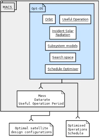
Opt-OS has a modular structure as seen in Figure2. Each element contained in Ops-OS contributes to the final result by providing a set of useful information to the optimiser, which can be used for calculating aspects of the satellite’s design.

Figure 2: Opt-OS modular structure.

A description of the modules comprising Opt-OS follows.

2.3.1 Orbit and useful operation

faster computation yet lower schedule flexibility. Whereas finer grained orbits lead to increased computational effort yet finer schedule control. A trade-off has to be made depending on the mission objectives and computational resources available. The useful operation module calculates the useful operation timeslot per subsystem throughout the mission timeline, based on the available subsystems onboard as well as the mission requirements. That way, an initial operations plan OPmax is formed

corresponding to the maximum useful operation time for every subsystem on-board.

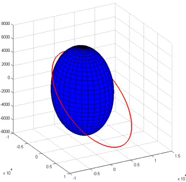
Figure 3: An example of a single orbital revolution for the chosen orbit with: a- 9105.6 km,e- 0.2444, i- 34.9398 ◦, RAAN - 110.4872 ◦,ω - 90◦, Mo

-130.42◦. Based on the aforementioned orbital ele-ments and the mission requireele-ments, the maximum useful operation time of each subsystem per revolu-tion is calculated.

2.3.2 Incident Solar Radiation

The incident solar radiation module performs ana-lytical calculation of the intensity of direct solar ra-diation at any point of the satellite’s surface. The solar radiation characteristics including the irradi-ance vector are calculated, contributing to the final calculation of the satellite solar array power output at any given time instance throughout the satellite orbit. This module can also be used for perform-ing satellite thermal analysis, which can be used for validating the mission requirements and design or imposing design constraints.

2.3.3 Subsystem models

The subsystem models module comprises analytical models of all vital subsystems on-board the satellite, namely Attitude Control Subystem (ACS), Power subsystem, Harness, Command & Data Handling (C& DH), Thermal, Propulsion (PROP). Based on a specific set of inputs, each model can output the basic physical and electrical characteristics of each subsystem as well as design characteristics such as the solar array area, the antenna type, the downlink datarate and so on.

Model inputs are divided into two categories: Design parameters andEnvironmental parameters. The de-sign parameterscan be decided by the designer with confidence or with uncertainty, depending on the ex-perience and previous knowledge on the respective design field. For instance the battery and solar cell type onboard the satellite can be considered part of the design parameters, as these choices depend on the designer’s discretion. Environmental param-eters cannot be decided, they are considered fixed due to environmental constraints. For example the solar flux is considered an environmental parameter since it does not depend on the designer

2.3.4 Search space

Based on the available subsystems on-board, a 2-dimensional search space is formed representing all the possible satellite operating states (Y-axis) during each timestep throughout the satellite mission time (X-axis) as seen in Figure5.

Figure 5: Opt-OS search space. X-axis represents the mission timeline in discrete timesteps, Y-axis represents all possible subsystem operation combi-nations in Boolean truth values.

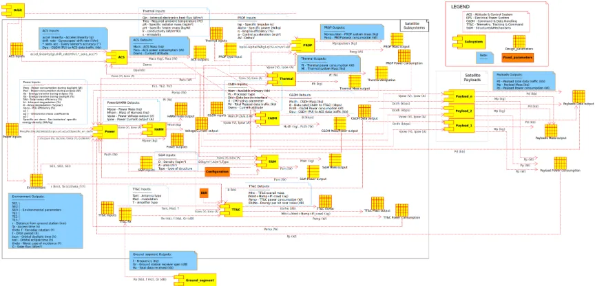
Figure 4: Full satellite blueprint based on analytical subsystem modelling. Each subsystem required a specific set of inputs, producing the basic electrical and physical subsystem characteristics amongst their outputs.

’subsystemOFF’ state whereas 1 corresponds to the ’subsystem ON’ state. The mission timeline is rep-resented as a set of discrete timestepsnof equal du-ration. The search space is of size (2S_{·n), with S}

being the number of available subsystems on-board the satellite.

2.3.5 Schedule Optimiser

The schedule optimiser is based on an Ant Colony System [6, 7, 8, 9, 10] inspired algorithm, designed to perform automated optimal operations scheduling according to the available resources on-board as well as the constraints imposed by environmental or tech-nical parameters. A colony of digital agents performs stochastic exploration of the search space, aiming at finding the optimal route corresponding to the opti-mal operations schedule, setting the maximum pos-sible operation time per subsystem as objective. The main satellite constraints are the power availability on-board as well as target visibility (e.g ground sta-tion visibility). The power availability constraint dictates the maximum amount of subsystems that can be kept ON at any time instant whereas the tar-get visibility constraint dictates individual subsys-tem characteristics such as the minimum datarate al-lowing the satellite to downlink each full data packet during a single transmission session.

Initially the algorithm’s parameters are set. The ants start exploring the search space, forming pos-sible optimal pathways. Once all ants comprising a colony reach the end, each pathway’s corresponding

Algorithm 2Schedule optimiser algorithm Set values form, α, ρ, ξ, Imax

Calculateτ0 using Eq. (6)

Define candidate listJi ∀i∈[search space] whileImaxnot met do

Place ants on source fork = 1:mdo

Retrieveτlj with l∈Jik

Decide nextjk _{using Eq. (7)}

Perform a local pheromone update on edgeij using Eq. (8)

if all ants have reached sinkthen break

end if end for

Calculate the quality of all tours Qk _using

Eq. (9)

FindQ+ _{using Eq. (10)}

Perform a global pheromone update onQ+

us-ing Eq. (11)

quality is measured, the best quality pathway, Q+_,

is enhanced with pheromone and all ants are placed back to the starting point where they initiate a new search. This iterative process continues until the op-timisation termination criterion, Imax, is met,

forc-ing the optimisation cycle to end. A more detailed description of the steps included in Algorithm 2 is found below.

- Set values for the number of antsmcomprising a colony, the pheromone influence parameterα, the global pheromone evaporation parameterρ, the local pheromone evaporation parameter ξ and the maximum number of iterations allowed Imax.

- Distribute a uniform layer of initial pheromone, τ0, on all edges comprising the search space. It

has been found [15] that a good convention for setting the initial pheromone levelτ0 is

τ0=C−1 (6)

whereChere is the mean of the total power con-sumption of all subsystems on-board the satel-lite throughout the mission timeline we exam-ine.

The initial pheromone level should allow enough iterations to take place, giving the ants enough time to converge towards an optimal solution. Care should be taken not to set the τ0 level

very high or very low though. A very high τ0

will cancel the effect of pheromone deposition during global pheromone update at the end of each iteration, leading to an increased number of iterations before converging to a good quality solution. On the other hand, a very lowτ0 will

lead the exploration process to a halt as soon as the search space pheromone level reaches zero. Since the next ant move depends on the proba-bility distribution deriving from Eq. (7), allow-ingτil(withl ∈Jik) to reach zero will result in

pk

ilequal to zero hence antkwill stop exploring.

- Define the candidate list ,Ji, of every node in

the search space withi∈[search space]. - While the optimisation termination criterion

,Imax, is not met

- Place all ants on source

- For all the ants ,m, of the colony

- Decide on the next ant step ,jk_{, using a variant}

of the probabilistic part of the pseudo-random

proportional rule

pk_ij = [τij]

α

P

l∈Jk i[τil]

α (7)

whereτij is the pheromone level of edgeij,αis

a positive weight parameter.

The next node is selected usingstochastic sam-pling also known as roulette wheel selection method. Utilising a weighted sample selection process, each ant chooses its next step accord-ingly. Higher probabilities within the proba-bility distribution pk

il acquire a bigger weight,

corresponding to a larger area on the roulette wheel. This leads to a biased selection favour-ing the choice of nodes correspondfavour-ing to higher probabilities within the distributionpk

il.

- Perform a local pheromone update on edge ij after each ant move.

τij(t)←(1−ξ)·τij(t) +ξ·τ0(t) (8)

where i, j are the nodes comprising edge ij that was just visited by ant k, ξ is the local pheromone evaporation rate parameter, τ0 is

the initial pheromone trail value occurring from Eq. (6)

- If all ants reached the end, break the loop in order to proceed to measuring the tours’ quality. - Calculate the qualityQk _{of every path formed.}

Qk=Tk∩OPmax (9)

whereTkis the path that antkformed through-out this iteration and OPmax is the maximum

useful operation period for all subsystems on-board

- Find the best-so-far solution qualityQ+_.

Q+=max(Q) (10)

- A global pheromone update is performed onQ+

τij(t)←(1−ρ)·τij(t) +ρ·∆τij(t) (11)

where ij are all the edges comprising Q+, ρ is the global pheromone evaporation parameter and the solution quality is calculated based on

∆τ ij(t) =ρ· Q

+

10|M agnt0|+|M agnρ|_·P

where Q+ _{is the best-so-far solution quality,}

|M agnτ0|is the absolute value of the magnitude

of the initial pheromone level τ0, |M agnρ| is

the order of magnitude of the global pheromone evaporation parameter ρandPpeak is the peak

power consumption found inOPmax.

- Once the optimisation criterion ,Imax, is met,

end the optimisation cycle.

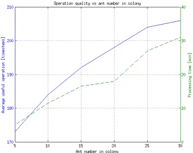
Two important factors have significant influence over the quality of the optimiser’s solution as well as the computational effort, namely the number of ants ,m, per colony and the global pheromone evapora-tion parameter ,ρ. As seen in Figure 6, a higherm can improve the solution quality for the same num-ber of iterations. As expected in serial agent-based processes, the computational time increases with the number of ants.

Figure 6: Opt-OS solution quality versus processing time as a function of ants per colony. TheImaxwas

set to 1000 iterations. Maximum feasible solution quality is 206.

The global pheromone evaporation parameterρ in-fluence as seen in Figure 7 is noteworthy. A lower ρ allows the ants to explore the search space more freely avoiding being trapped in local optima too eas-ily. The enhanced exploration leads to a higher com-putational time as more options need to be explored, yet a significantly improved solution quality.

3 TEST CASE

In this section, we demonstrate the flexibility of Opt-OS by utilising it in the following proposed satellite design integrated approach described in Figure8. A simple generic satellite is considered, containing an

Figure 7: Opt-OS solution quality versus processing time as a function of global pheromone evaporation. TheImaxwas set to 1000 iterations. Themwas set

to 10 ants.

Electrical Power Subsystem (EPS) and a Telecom-munications subsystem as described in [16].

The design process is performed by two enclosed loops, namely the Inner loop (Opt-OS) and the Outer loop (MACS). The Inner loop models the satellite and derives its optimal operations sched-ule as described above. The Inner loop’s output comprises three main quantities, the total satellite mass ,Mtot, the satellite downlink datarate ,Drate

and the optimal mission operations schedule qual-ity ,Q+, i.e the cardinality of the intersection be-tween the maximum useful operation period ,OPmax,

and the current optimised operations schedule based on the quality criterion of Eq. 9. Depending on the mission requirements, the Inner loop can output more results like for example the onboard databus datarate and so on.

The Outer loop comprises MACS, a stochastic multi-objective optimization algorithm combining together a number of heuristics as described in [5]. Using a combination of heuristics, a population of agents explores the search space both in a global fash-ion and around the neighbourhood of each agent. The heuristic driven optimisation process is comple-mented with a local and global archive. The algo-rithm comprises eight basic steps namely Initializa-tion, CollaboraInitializa-tion, SelecInitializa-tion, Filtering, Repulsion, Local actions, Hyperrectangle update, Archive up-date and the Stopping rule.

Figure 8: Integrated system-operations design ap-proach.

place where the satellite design parameters are opti-mised depending on the objectives set. In this test case the objectives set are the following: min(Mtot)

whilemax(Drate) andmax(Q+).

The Outer loop finally outputs a Pareto set of points as seen in Figure 9, representing optimisers. Each point represents a vector of optimal subsystem de-sign parameters leading to a full optimal satellite design.

Figure 9: Pareto set of optimisers. Each point cor-responds to a full optimal satellite design. Thicker points correspond to higher satellite masses.

The table below contains an example of 5 opti-mal satellite design parameter sets corresponding to

Pareto points lying in the lower mass spectrum. Table 1: An example of five optimal design param-eter sets lying in the lower mass spectrum of the Pareto set.

1 2 3 4 5

TTC design parameters

f [GHz] 4 3.87 4.21 4 5.15

Ant 2 2 2 2 2

M od 0.02 0.46 0.3 0.02 0.28 T 0.44 0.53 0.56 0.44 0.69 T e[K] 91.49 91 86.91 91.49 93.77 F [dB] 12.37 11.6 13.6 12.37 10.24 T et[K] 49.62 53.57 49.62 66.45 77.58 F t[dB] 12.79 13.15 12.21 12.79 13.78 T ant[K] 50.98 66.1 62.66 62.45 69.13 nt 0.62 0.77 0.63 0.75 0.55

Lc[m] 0.3 0.3 0.3 0.3 0.3

EPS design parameters SAt 0.27 0.29 0.25 0.27 0.32

Xe 0.63 0.64 0.62 0.63 0.6

Xd 0.8 0.85 0.82 0.8 0.81

Id 0.85 0.86 0.7 0.85 0.83 SM

[kg/m2_{] 2.64 1.36 2.13 2.64 2.72} npcu 0.89 0.9 0.86 0.89 0.9

SED

[W h/kg] 123.3 77.15 63.81 123.3 183.5 V drop 0.04 0.03 0.04 0.04 0.04

The TTC design parameters correspond to: f - Transmission Frequency [GHz], Ant - Antenna Type [1 - Horn, 2 - Parabolic reflector],Mod- Mod-ulation (Treating the modMod-ulations range as continu-ous gives the designer the ability to choose any type of existing or possible future modulations in the form of real numbers interpolated over the modulation range [14]), T - Amplifier Type (Treating the am-plifier types range as continuous gives the designer the ability to choose any type of existing or possible future amplifier types in the form of real numbers in-terpolated over the amplifier types range [14]),Te -Amplifier noise [K],F- Receiver Noise Figure [dB], Tet - Amplifier noise [K], Ft - Transmitter Noise Figure [dB],Tant- Antenna Noise Temperature [K], nt- Antenna efficiency [%],Lc- Antenna character-istic length [m].

The EPS design parameters correspond to: SAt -solar cell efficiency [%],Xe- Energy transfer during eclipse [%],Xd- Energy transfer during daylight [%], Id - Inherent degradation [%], SM - array specific mass [kg/m2_{], npcu - PCU efficiency [%], SED}

Vdrop- Maximum permissible bus voltage drop [%].

4 CONCLUSION

In this paper, a flexible optimal operations schedul-ing approach is proposed. A modular tool is presented, offering automation of the operations scheduling process while enhancing the robustness of the operations schedule. The tool, namely Opt-OS, comprises a set of modules modelling the satellite and its environment as well as a nature-inspired op-timiser outputting the optimal operations schedule on the spot. Opt-OS can be used in order to alle-viate the workload of mission operations teams, en-hance the robustness of the operations schedule, de-vise emergency operations plans. All in all, Opt-OS aims at maximising the use of the satellite through-out each mission timeline instant.

Furthermore, Opt-OS can be used as the basis of an integrated automated optimal satellite design ap-proach, where initially an optimal operations sched-ule is designed followed by a set of optimal satellite designs utilising this operations schedule. This auto-mated approach can offer enhanced robustness over the classical design approach while outputting a cost effective design produced in a timely fashion, thus making space accessible to a wider spectrum of in-stitutions with lower budgets.

5 ACKNOWLEDGEMENTS

The author would like to thank Mr. Alasdhair Beaton and Mr. Massimo Vetrisano for their valu-able contribution to this work. This research has been partially conducted using the University of Strathclyde High Performance Computer (HPC).

REFERENCES

[1] Harland, D. M. and Lorenz, R. D.,Space Systems Failures, Disasters and Rescues of Satellites, Rock-ets and Space Probes, Springer and Praxis, 2005.

[2] “Mars Climate Orbiter Mishap Investigation Board Phase I Report,” Tech. rep., 1999.

[3] “Lewis Spacecraft Mission Failure Investigation Board: Final Report,” Tech. rep., 1998.

[4] Sims, M. R.,Beagle-2, Lessons Learned and Man-agement and Programmatics, University of Leices-ter, 2004.

[5] Vasile, M. and Locatelli, M., “A hybrid multiagent approach for global trajectory optimization,” Jour-nal of Global Optimization, Vol. 44, No. 4, 2009, pp. 461–479.

[6] Dorigo, M. and Stuetzle, T.,Ant Colony Optimiza-tion, MIT Press, 2004.

[7] Dorigo, M. and Gambardella, L., “Ant Colony Sys-tem: A Cooperative Learning Approach to the Traveling Salesman Problem,” IEEE Transaction on Evolutionary Computation, Vol. 1, No. 1, 1997, pp. 53–66.

[8] Dorigo, M. and Gambardella, L., “Ant Algorithms for Discrete Optimisation,” Artificial Life, MIT Press, Vol. 5, No. 2, 1999.

[9] Bonabeau, E., Dorigo, M., and Theraulaz, G.,

Swarm Intelligence From Natural to Artificial Sys-tems, Santa Fe Institute: Studies in the Sciences of Complexity, Oxford University Press, 1999.

[10] Ostfeld, A., editor, Ant Colony Optimization -Methods and Applications, InTech, 2011.

[11] Papadimitriou, C. H., “The Euclidean travelling salesman problem is NP-complete,” Theoretical Computer Science, Vol. 4, No. 3, 1977, pp. 237 – 244.

[12] Karlson, P. and Luscher, M., “Pheromones: a New Term for a Class of Biologically Active Substances,”

Nature, , No. 183, 1959, pp. 55–56.

[13] Cover, T. M. and Hart, P. E., “Nearest Neighbor pattern classification,”IEEE Transactions on Infor-mation theory, Vol. IT-I3, No. 1, 1967, pp. 21–27.

[14] Larson, W. J. and Wertz, J. R.,Space Mission Anal-ysis and Design, Microcosm Press and Kluwer Aca-demic Publishers, 2005.

[15] Komninou, E., Vasile, M., and Minisci, E., “Opti-mal power harness routing for s“Opti-mall-scale satellites,” October 2011.