Computing the set of Epsilon-efficient solutions in multiobjective space mission design

Computing the Set of epsilon-efficient Solutions in

Multi-Objective Space Mission Design

Oliver Sch¨

utze

_{Massimiliano Vasile}

Carlos A. Coello Coello

∗‡_{CINVESTAV-IPN, Av. IPN No. 2508, San Pedro Zacatenco, 07360, Mexico}

†_{University of Strathclyde, 75 Montrose Street G1 1XJ, Glasgow, United Kingdom}

In this work, we consider multi-objective space mission design problems. We will start from the need, from a practical point of view, to consider in addition to the (Pareto) opti-mal solutions also nearly optiopti-mal ones. In fact, extending the set of solutions, for a given mission, to those nearly optimal significantly increases the number of options for the deci-sion maker and gives a measure of the size of the launch windows corresponding to each optimal solution, i.e. a measure of its robustness. Whereas the possible loss of such approx-imate solutions compared to optimal—and possibly even ‘better’—ones is dispensable. For this, we will examine several typical problems in space trajectory design—a bi-impulsive transfer from the Earth to the asteroid Apophis and two low-thrust multi-gravity assist transfers—and demonstrate the possible benefit of the novel approach. Further, we will present a multi-objective evolutionary algorithm which is designed for this purpose.

I.

Introduction

In a variety of applications in industry and finance a problem arises that several objective functions have to be optimized concurrently leading tomulti-objective optimization problems (MOPs). For instance, in space mission design, which we address here, about fifty percent of the cost of a mission is due to the space segment, including launch, and fifty percent due to the ground segment, i.e. the cost of operations. The cost of the space segment, in particular of the launch, can be related to the mass of the spacecraft and to the total ∆v(total variation of the linear velocity of the spacecraft) required to reach a given target. The total ∆v has a direct impact on the mass of propellant onboard the spacecraft and on the required launch capabilities. In other words, the higher the ∆v and the mass of the spacecraft, the higher the cost of the launch. Of course, the launch capabilities are limited, therefore for every spacecraft mass there is an upper limit on the possible ∆v, in this paper, however, we are not considering that limit. The cost of operations is directly related to the total mission time, and in the case of an interplanetary transfer to the total time of flight. Therefore, for the optimal design of a generic interplanetary trajectory we can identify two objective functions: time of flight and total ∆v (or total propellant consumption).3, 19, 21, 24

The quality of a solution in a MOP is generally defined by its Pareto optimality, i.e. a solution is Pareto optimal if no other solution is better over all the objective values. The set of Pareto optimal solutions form a Pareto set in the parameter space and a Pareto front in the objective space. As shown later in this paper and also by Vasile,22 _{the Pareto set can cover only a small portion of the parameter space, corresponding to}

a limited number of launch dates. During the design of a space mission, in particular in the early phase, it would be desirable, instead, to have also the solutions in the neighborhood of the optimal ones. A knowledge of the neighboring solutions will help in the identification of the extension of the launch window associated to each optimal solution, i.e. the range of possible launch dates for which both the total ∆v and the time of flight are below a given threshold. In other words, a knowledge of the neighboring solutions gives a measure of the robustness of an optimal solution. Note that designing for the suboptimal points increases

∗_{Associate Professor, Department of Computer Science}

the reliability of the mission since it gives the freedom to deviate from the chosen design point with little or no penalty. This holds true also for Pareto optimal solutions. It is therefore desirable to have a whole range of nearly Pareto optimal solutions for each Pareto point. Furthermore, it would be desirable to extend as much as possible the number of launch opportunities.

As a motivating example we consider the MOP in Section IV.C, which corresponds to the design of a low-thrust multigravity assist trajectory from the Earth to Mercury following the sequence Earth – Venus – Mercury. Let us consider the two pointsxi with imagesF(xi), i= 1,2:

x1 = (782, 1288, 1788) , F(x1) = (0.462, 1001.7)

x2 = (1222, 1642, 2224), F(x2) = (0.463, 1005,3)

The two objectives are the propellant mass fraction—i.e., the portion of the vehicle’s mass which does not reach the destination—and the time of flight (in days). In the domain, the first parameter is of particular interest: it determines the departure time from the Earth (in days after 01.01.2000), i.e., the launch time of the mission. F(x1) is less thanF(x2) in both components, and thus,x1 can be considered to be ‘better’

thanx2(x1is said todominatex2). However, the difference in image space is small: the mass fraction of the

two solutions differs by 0.001 which makes 0.1% of the total mass, and the flight time differs by four days for a transfer which takes almost three years. In case the DM is willing to accept this deterioration, it will offer him/her a second choice in addition to x1 for the realization of the transfer: while the two solutions offer

‘similar’ characteristics in image space this is not the case in the design space since the starting times for the two transfers differ by 440 days. The two solution, therefore, represent two distinct launch opportunities.

In this case, the identification of two solutions increases the reliability of the design, because one solution can become the baseline and the other can serve as back-up, with almost identical cost. This paper will show the benefits of considering, in addition to the Pareto optimal trajectories, also the set of approximate (or nearly optimal) solutions. Furthermore, it will present one way to compute this enlarged set of interest with a reasonable computational effort through a novel evolutionary algorithm based on a particular archiving technique.

The field of evolutionary multi-objective optimization is well-studied and multi-objective evolutionary algorithms (MOEAs) have been successfully applied in a number of domains, most notably engineering applications.2 _{Approximate solutions in multi-objective optimization have been studied by many researchers}

so far,12, 13, 26_{however, the only studies which deal (albeit theoretically) with the computation of the entire}

set of approximate solutions have been undertaken by Sch¨utze et al.18, 19 _{A first attempt to investigate the}

benefit of considering approximate solutions in space mission design has been done by Vasile and Locatelli,23

albeit for the single-objective case.

The additional consideration of approximate solutions in multi-objective space mission design problems is new and will be addressed in this paper (a preliminary study of this paper can be found in Sch¨utze et al.20_).

Crucial for this approach is the efficient computation of the enlarged set of ‘optimal’ points (the second scope of this paper) since in many cases the ‘classical’ multi-objective approach is a challenge itself. For this, we will propose an algorithm which is modeled on the basis of theǫ-MOEA6 _{and which is adapted to}

the current context. Note that ‘classical’ archiving/selection strategies—e.g., the ones reported by Hanne,9

Rudolph & Agapie,16 _{Laumanns et al.}12 _{and Knowles & Corne,}11_{or the ones most state-of-the-art MOEAs}

such as NSGA-II4 _{use—store sets of mutually non-dominating points (which means that e.g. the pointsx} 1

andx2in the above example will never be storedjointly). That is, these selection mechanisms—though they

accomplish an excellent job in approximating the efficient set—can not be adopted for our purposes. The remainder of this paper is organized as follows: in Section II, we give the required background which includes the statement of the space mission design problem under consideration. In Section III, we propose a new genetic algorithm for the computation of the set of approximate solutions and present further on in Section IV some numerical results. Finally, we conclude in Section V.

II.

Background

II.A. Multi-Objective Optimization

In the following we consider continuous multi-objective optimization problems

min

x∈Q{F(x)}, (MOP)

where the domainQ⊂R

n _{is compact andF :Q→}

R

k _{is defined as the vector of the objective functions}

F(x) = (f1(x), . . . , fk(x)), (1)

and where each objective fi : Q → R is continuous. The concept of optimality we use here was first

introduced by Pareto:14

Definition 1 Letv, w∈Q. Then the vectorvisless thanw(v <pw), ifvi< wi for alli∈ {1, . . . , k}. The

relation ≤p is defined analogously. y∈Qis dominatedby a point x∈Q (x≺y) with respect to (MOP) if F(x)≤pF(y)andF(x)6=F(y). x∈Qis called aPareto optimal pointorPareto pointif there is noy∈Q

which dominatesx.

The set of all Pareto optimal solutions is called thePareto set(denoted byPQ). The image of the Pareto set F(PQ) is called the Pareto front. We now define another notion of dominance which we use to define approximate solutions.

Definition 2 Let ǫ= (ǫ1, . . . , ǫk)∈R

k

+ andx, y∈Q.

(a) xis said to ǫ-dominatey (x≺ǫy) with respect to (MOP) ifF(x)−ǫ≤pF(y)andF(x)−ǫ6=F(y).

(b) xis said to−ǫ-dominatey (x≺−ǫy) with respect to (MOP) ifF(x) +ǫ≤pF(y)andF(x) +ǫ6=F(y).

The notion of−ǫ-dominance18_{is, of course, analogous to the ‘classical’ǫ-dominance relation}13_{but with}

a value ˜ǫ∈R

k

−. However, we highlight it here since we use it to define our set of interest:

Definition 3 Denote by PQ,ǫ the set of points in Q⊂R

n _{which are not −ǫ-dominated by any other point}

inQ, i.e.,

PQ,ǫ:={x∈Q| 6 ∃y∈Q:y≺−ǫx}. (2)

The setPQ,ǫ contains allǫ-efficient solutions, i.e., solutions which are optimal up to a given (small) value of ǫ. Fig. 1 gives two examples.

Figure 1. Two different examples for setsPQ,ǫ. At the left, we show the case fork= 1and in parameter space with PQ,ǫ= [a, b]∪[c, d]. Note that the image solutionsf([a, b])are nearly optimal (measured in objective space), but that the

entire interval[a, b]is not ‘near’ to the optimal solution which is located within[c, d]. At the right, we show an example fork= 2in image space,F(PQ,ǫ)is the approximate Pareto front.

Algorithm 1 gives a framework of a generic stochastic multi-objective optimization algorithm, as the one we consider in this work. Here, Q ⊂ R

n _{denotes the domain of the MOP, P}

j the candidate set (or population) of the generation process at iteration stepj, and Aj the corresponding archive.

Algorithm 1Generic Stochastic Search Algorithm

1: P0⊂Qdrawn at random 2: A0=ArchiveU pdate(P0,∅) 3: forj= 0,1,2, . . .do

4: Pj+1=Generate(Pj)

5: Aj+1 =ArchiveU pdate(Pj+1, Aj)

6: end for

Definition 4 Let u, v∈R

n _{and A, B ⊂}

R

n_{. The maximum norm distance d}

∞, dist(·,·), anddH(·,·) are

defined as follows:

(a) d∞(u, v) := max

i=1,...,n|ui−vi|

(b) dist(u, A) := inf

v∈Ad∞(u, v)

(c) dist(B, A) := sup u∈B

dist(u, A)

(d) dH(A, B) := max{dist(A, B),dist(B, A)}

Note that dist is not symmetric. For instance, for A= [0,1] and B = [0,2] it is dist(A, B) = 0 (since A⊂B) anddist(B, A) = 1.

Sch¨utze et al.19 _{showed that, under certain (mild) conditions on the setP}

Q,ǫ of the MOP and under the assumption

∀x∈Qand∀δ >0 : P(∃l∈N : Pl∩Bδ(x)∩Q6=∅) = 1, (3)

onGenerate() the Algorithm 1 equippped with Algorithm 2 as archiver generates a sequence of archives Aiwhich converges with probability one toward an approximation of the set of interest (hereby,P(A) denotes the probability for eventA). More precisely, there exists with probability one anl0 ∈ Nsuch that for all

l≥l0:

dH(F(PQ,ǫ), F(Al))≤max(∆, dist(F(PQ,ǫ+2∆), F(PQ,ǫ)), (4)

where ∆<mini=1,...,kǫiand ∆∗are parameters used to determine the granularity of the approximation: the archive ensures (line 3 of Algoritm 2) that the minimal difference between two archive images is bounded, i.e.,

kF(a1)−F(a2)k∞≥∆∗, ∀a1, a2∈Al:a16=a2, ∀l∈N, (5)

resulting in a natural ‘spread’ of the archive entries by which it follows that no additional spreading mechanisms such as niching techniques7, 8 are required in a MOEA which is equipped with this archiver. ∆∗_{<∆ is required for theoretical purposes, in practise ∆}∗_{= ∆ can be chosen, for a thorough discussion we}

refer to Sch¨utze et al.19

II.B. The Design Problems

In the following we will analyze a few examples taken from two classes of typical problems in space trajectory design: a bi-impulsive transfer from the Earth to the asteroid Apophis, and two low-thrust multi-gravity assist transfers from the Earth to a planet.

Bi-impulse Problem _{For the bi-impulsive case, the propellant consumption is a function of the velocity}

change, or ∆v,1 _{required to depart from the Earth and to rendezvous with a given celestial body. Both}

Algorithm 2A:=ArchiveU pdatePQ,ǫ(P, A0,∆)

Require: population P, archiveA0, ∆∈R+, ∆

∗_∈(0,∆)

Ensure: updated archiveA

1: A:=A0

2: for allp∈P do

3: if 6 ∃a1∈A: a2≺−ǫpand6 ∃a2∈A: d∞(F(a2), F(p))≤∆∗ then 4: A:=A∪ {p}

5: for alla∈Ado

6: if p≺−(ǫ+1∆)athen 7: A:=A\{a}

8: end if

9: end for

10: end if

11: end for

to the target. The second change in velocity, or ∆v2, is then used to inject the spacecraft into the target’s

orbit.

The two ∆v’s are a function of the positions of the Earth and the target celestial body at the time of departure t0 and at the time of arrivaltf =t0+T, where T is the time of flight. Thus, the MOP under

consideration reads as follows:

minimize:   

∆v1+ ∆v2

T

(6)

MLTGA Problem _{It is here proposed to use a particular model for multiple gravity assist low-thrust}

trajectories (MLTGA). Low-thrust arcs are modeled through a shaping approach based on the exponential sinusoid proposed by Petropoulos et al.15 _{The spacecraft is assumed to be moving in a plane subject to the}

gravity attraction of the Sun and to the control accelerationF= [F cosα, F sinα]T _{of a low-thrust propulsion} engine. The dynamic equations governing the motion of the spacecraft can be written in polar coordinates as follows:

¨

r−rθ˙2+ µ

r2 =F sinα

1 r

d dt(r

2_{θ) =˙ F cosα}

whereαis the thrust steering angle measured clockwise from the axis perpendicular torin the direction of motion. For this particular dynamics Petropoulos proposed to use the following shaping function for the radius as a function of the polar angleθ.

r=k0ek1sin(k2θ+φ)

Then, if the thrust vector is aligned with the velocity vector, the flight path angle γ and the thrust steering angleαare equal. Ifγ=α, the thrust history and the polar angle history are uniquely determined and the control acceleration is given by:

F= µ r2

tanγ 2cosγ

1 tan2_γ+k

1k22s+ 1

− k

2

2(1−2k1s)

(tan2_γ+k

1k22s+ 1)2

(7)

with the time variation of the true anomaly given by:

˙ θ2₌µ

r3

₁

tan2_γ+k

1k22s+ 1

(8)

tanγ =k1k2cos(k2θ+φ) (9)

with s= sin(k2θ+φ). Now, by solving the following integral:

∆t=

Z _dθ

q µ r3

1

tan2_γ+k1k2 2s+1

(10)

one can compute the actual time of flight.

The exponential sinusoid expresses the variation of the radius as a function of the polar angle θ and depends on three shaping parameters k0, k1, k2 plus a phase parameter φ. By fixing the initial and final

radius forθ= 0 and theta= ¯θrespectively:

r1=k0ek1sin(φ)

r2=k0ek1sin(k2 ¯

θ+φ) (11)

two of the three parameters can be computed as a function of the others.

The two position radii and the angular difference ¯θbetween the departure and the arrival points can be computed from the ephemerides of the departure and arrival planets or other celestial bodies (in this work we used analytical ephemerides). In this case it is normally required that the transfer trajectory going from one planet to the other is flown in a given timeT. This implies that the actual time of flight must be equal to the required time of flight in order to have a physical solution:

∆t−T = 0 (12)

If now this time constraint is solved a third parameter can be determined and the exponential sinusoid becomes a single valued function (for more details on the solution of (12) please refer to Izzo10_).

In this form, given the transfer time and the two position vectors at the beginning and at the end of the transfer we can compute the velocities at the two extremal points and the thrust profile. Since only one shaping parameter is free it is not possible to optimize the value of the velocities at the boundaries plus the thrust profile but the problem is equivalent to the Lambert’s problem for conic arcs.

Furthermore, some analysis15 _{reveals that the exponential sinusoid gives physical solutions whenever}

k1k22<1. This limit will be used in the remainder of this paper to limit the values of the shaping parameter

k2.

Gravity assist manoeuvres are modeled with a linked-conic approximation: the manoeuvre is instanta-neous (i.e. no variation in the position of the spacecraft) and produces a deflection of the planetocentric velocity vector, the planet is reduced to a point mass with no gravity, the deflection angleβswingis a function of the mass of the planet and of the incoming velocity, such that:

e

vT_inevout=−evi2cosβswing (13)

and

βswing= 2 arccos

µp e v2

inrp+µp

(14)

where µp is the gravity constant of the swing-by planet, evin and veout are the planetocentric incoming and outgoing velocity vectors andrp is the radius of the pericentre of the swing-by hyperbola.

Since the value of the velocities at the boundaries is not completely free, to give an incoming velocity vector is not possible, in general, to match every possible outgoing velocity vector.

A match can be obtained by inserting a ∆V correction at the pericentre of the hyperbola of the swing-by. This model will be called powered swing-by model or powered swing-by in the following.

Here we describe the bi-objective optimization problem we consider in the sequel. The two objectives are the propellant mass fraction and the flight time which result by a given trajectory.

minimize: J(y) subject to: rp≥rmin

(15)

the complete solution vector is then defined as follows:

y= [t0, T1, k2,1, n1, ..., Ti, k2,i, ni, ..., TN, k2,N, nN]T (16)

Wherek2,i is the i-th shaping parameter for the exponential sinusoid and ni the number of revolutions around the Sun. The objective functionJ is then defined as follows:

J= 1−e−(

∆VGA+∆V₀ g0Isp1 +

∆VLT

g0Isp2) (17)

where ∆VGA is the sum of all the ∆V s (variation in velocity) required to correct every gravity assist manoeuvre, ∆V0is the departure manoeuvre, while ∆VLT is the sum of the total ∆V of each low-thrust leg. The two specific impulses Isp1 and Isp2 are respectively for a chemical engine and for a low-thrust engine

andg0 is the gravity acceleration on the surface of the Earth.

For the tests in this paper, we used Isp1 = 315s and Isp2 = 2500s. Note that, the computation of a

transfer arc with the exponential sinusoid does not require the time history of the mass of the spacecraft. The time history of the mass would be required to compute the actual thrust profile along the transfer arc. The integration of (7), instead, gives directly the ∆v due to the low-thrust propulsion.

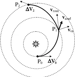
The objective function (17) is particularly appealing because it has values ranging from 0, best transfer, to 1, worst transfer. In addition, the impulsive ∆v and the low-thrust ∆v are weighted in such a way that the use of low-thrust is favored with respect to the use of the impulsive corrections. Note that the scope of this paper is not to demonstrate the suitability of the exponential sinusoid model for the design of MLTGA trajectories but rather to demonstrate the benefit of the additional use of approximate solutions. The overall process for the composition of a MLTGA trajectory with the exponential sinusoid model can be summarized with the following steps (see Fig. 2):

• For each departure datet0andN legs with transfer timesT= [T1, ..., Ti, ..., TN]T

• Compute a low-thrust arc through the exponential sinusoid model from planet ito planet i+ 1 (see the transfer from A to B as an example in Fig. 2)

• Compute the incoming heliocentric velocity vector vin and the corresponding planetocentric velocity vectorvein

• Compute a low-thrust arc through the exponential sinusoid model from planet i+ 1 to planet i+ 2 (see the transfer from B to C as an example in Fig. 2)

• Compute the required heliocentric outgoing velocity vectorvrout and the corresponding required plan-etocentric velocity vectorverout

• Compute the achievable planetocentric outgoing velocity vector_evaoutwith pericenter radiusrp≥rmin

• Ifv_eaout6=evrout compute the matching ∆Vi at the pericentre of the hyperbola

• Compute the launch impulsive manoeuvre ∆V0

• Compute the arrival impulsive manoeuvre ∆VN

• Compute the the low-thrust ∆VLT

• Compute the sum of all ∆V’s

The arrival at planeticorresponds to a timeti=ti−1+Ti, therefore the final time at the end of the transfer istN, while the corrective ∆V’s are computed for all the indexes from 2 toN−1.

Figure 2. Composition of a whole MLTGA trajectory for the exponential sinusoid model

change is obtained through an impulsive manoeuvre at the boundaries of the low-thrust arc and included in ∆V0, ∆VN, or in the ∆VGA.

The second objective of the MOP which we address in this work is simply given by theflight timetN−t0

used for the selected trajectory. This objective is of great importance for the design process since the transfer can take several years.

Thus, the MOP under consideration reads as follows:

minimize:   

J(y)

tN −t0

subject to: rp≥rmin

(18)

III.

A MOEA for the Computation of

_P

Here, we present a novel evolutionary algorithm,PQ,ǫ-MOEA, for the computation of the set of approxi-mate solutions, and present further on some performance indicators which aim to measure the approximation quality of a given outcome set.

III.A. The Algorithm

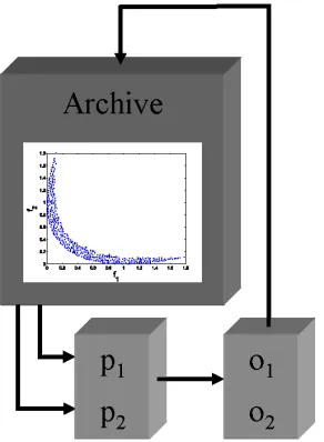
The evolutionary strategy, PQ,ǫ-MOEA, we propose here is a steady-state archive-based MOEA. In the beginning, the archiver is fed with randomly chosen elements from Q, where ArchiveUpdatePQ,ǫ is taken as archiver. In the i-th step of the algorithm two parent solutions p1 and p2 are chosen at random from

the current archiveAi from which the two offspring o1 and o2 are generated as follows: either crossover is

performed (with a given probabilitypc) or mutation is performed on both archive entries. The offspring is finally used to updateAileading to the new archiveAi+1 (see Algorithm 3 and Figure 3). For the numerical

results that we will present in the sequel we have used the Simulated Binary Crossover (SBX) and the Polynomial Mutation, respectively.5

Since the probability for mutation is positive in each step and the support of the density function of the Polynomial Mutation is positive on Q for each point x ∈ Q the general assumption on the generator (3) is fulfilled. Hence, PQ,ǫ-MOEA generates with probability one a sequence of archives Ai which converges toward an approximation of the set of interest (compare to the Section II or to Sch¨utze et al.19_).

The PQ,ǫ-MOEA has been modelled on the basis of ǫ-MOEA which has been proposed by Deb et al.6 Deb et al.6 _{note that}

‘..., it is observed that the steady-state MOEA is a good compromise in terms of convergence near to the Pareto-optimal front, diversity of solutions, and computational time.’

Algorithm 3PQ,ǫ-MOEA

1: P0⊂Qdrawn at random 2: A0:=ArchiveU pdatePQ,ǫ(P0,∅) 3: forl= 0,1,2, . . .do

4: choosep1, p2∈Alat random

5: perform generational operators onp1, p2 leading too1, o2 6: Al+1:=ArchiveU pdatePQ,ǫ({o1, o2}, Al)

7: end for

with a different archiver), and (ii) PQ,ǫ-MOEA does not use a population in addition to the archive. The latter is included inǫ-MOEA to prevent that the candidate set ‘collapses’ when inserting strongly dominating solutions (i.e., when an entire range of archive entries is dominated by an offspring o these are discarded from the archive—when using an elitism strategy and when heading for the Pareto front—which could result in a bad performance of the population-based approach due to the lack of candidate solutions in a certain region). We have observed that such a mechanism (and the related additional computational complexity) is not required when heading forPQ,ǫ. In fact, since in ArchiveUpdatePQ,ǫelements are discarded if they are

−(ǫ+ ∆)-dominated by an offspringo, the archiver is much more robust to such collapses.

So far, the only existing algorithm for the computation ofPQ,ǫ isPQ,ǫ-NSGA-II proposed by Sch¨utze et al.,20_{which is based on the well-known NSGA-II.}4 _P

Q,ǫ-NSGA-II uses the same ranking strategy as its base MOEA, and thus, the highest pressure of the population is taken toward the Pareto set. We have observed, however, that this could lead to problems whenPQ,ǫ contains connected components where the intersection with the Pareto set is empty (i.e., for each pointxin such a componentCthere exists an elementy6∈Csuch thaty≺x) since in that case such components can be overseen by the search strategy (see, for instance, the example in Section IV.A). Instead, the search should be performed bias-free on the entire set of approximate solutions, which was the motivation for developing the newPQ,ǫ-MOEA.

III.B. Performance Metrics

In order to assess the performance of an (evolutionary) algorithm, it is desirable to have a performance metric that measures the approximation quality of the outcome set. Since so far no such metric exists, we adapt here some established indicators for the classical multi-objective case to the current context. Whereas all (established) performance indicators for the treatment of classical MOPs are defined in objective space, we have to consider here in addition the approximation quality in parameter space since this is one important aspect when considering approximate solutions (see for instance the left example in Fig. 1).

Assume we are given the set PQ,ǫ analytically (or we are given a good approximation of it), then the approximation quality of a given (finite) archive A = {a1, . . . , al} can, for example, be measured by the Hausdorff distance:

dH(A, PQ,ǫ) =max(dist(A, PQ,ǫ), dist(PQ,ǫ, A)), (19)

where

dist(A, PQ,ǫ) = maxi=1,...,lminp∈PQ,ǫkai−pk, (20)

dist(PQ,ǫ, A) = maxp∈PQmini=1,...,lkai−pk (21)

If the value in (19) is 0, it means thatAis dense inPQ,ǫ(i.e., the closure ofAis equal toPQ,ǫ), and thus, A can be regarded as a perfect approximation. By this, it follows that small values ofdH in (19) indicate good approximations A. In case the value of dH is not small, however, a more detailed consideration is required. One can for instance consider instead of (19) the two values of (20) and (21) separately: (20) measures the convergence ofA toward PQ,ǫ while (21) gives an idea about the spread of the entries of A along the set of interest. One potential drawback of the indicators (20) and (21)—and hence also of (19)—is that single outliers can give a false impression on the approximation quality, a problem which is hard to overcome when using stochastic search algorithms. Instead, the distances can be averaged leading to the following alternatives to (20) and (21), respectively.

GDx(A) := 1 l

v u u tXl

i=1

(dist(ai, PQ,ǫ)2, (22)

IGDx(A) := 1 m

v u u t

m X

i=1

(dist(pi, A)2, (23)

where we assume that we are given an approximation of PQ,ǫ consisting ofm elements. These indica-tors are modifications of the Generational Distance25 _{and the Inverted Generational Distance}2 _{which are}

The above discussion is analog for a performance measure in objective space. The Hausdorff distance of the image ofAtoward the approximate Pareto frontF(PQ,ǫ) is given by

dH(F(A), F(PQ,ǫ)) =max(dist(F(A), F(PQ,ǫ)), dist(F(PQ,ǫ), F(A))), (24)

where

dist(F(A), F(PQ,ǫ)) = maxi=1,...,lminp∈PQ,ǫkF(ai)−F(p)k, (25)

dist(F(PQ,ǫ), F(A)) = maxp∈PQmini=1,...,lkF(ai)−F(p)k (26)

The averaged distances are as follows:

GDy(F(A)) := 1

l v u u tXl

i=1

(dist(F(ai), F(PQ,ǫ))2, (27)

IGDy(F(A)) := 1 m v u u t m X i=1

(dist(F(pi), F(A))2, (28)

Things change when no approximation of PQ,ǫ of the MOP is at hand since in that case no statements on the approximation quality in parameter space can be made (note that PQ,ǫ is based on the concept of

−ǫ-dominance which is defined in objective space), and we have to leave this issue for future research. For a comparison of two given outcome setsAandB in image space we found the following indicator useful

C−ǫ(A, B) :=

|{b∈B : ∃a∈A:a≺−ǫb}|

|B| , (29)

which is a straightforward extension of theset coverage metricsuggested by Zitzler & Thiele.27 _{Analogue to}

the original metric,C−ǫ(A, B) is an unsymmetric operator which aims to get an idea of the relative spread of the two solution sets.

IV.

Numerical Results

Here we present some numerical results coming from one academic problem and three different space mission design scenarios.

IV.A. An Academic Example

First, we consider an academic MOP in order to demonstrate the strength of the novel approach. The model is a modification of the one proposed by Rudolph et al.:17

F :R

2_→

R

2

F(x1, x2) = (x1−t1(c+ 2a) +a) 2_{+ (x}

2−t2b)2+δt (x1−t1(c+ 2a)−a)2+ (x2−t2b)2+δt

!

, (30)

where

t1= sgn(x1) min

|x1| −a−c/2

2a+c

,1

, t2= sgn(x2) min

|x2| −b/2

b ,1 , and

δt= (

0 fort1= 0 andt2= 0

0.1 else .

Usinga= 0.5,b= 5,c= 5 MOP (30) contains one global Pareto set

P0,0= [−0.5,0.5]× {0} (31)

P−1,−1= [−6.5,−5.5]× {−5}

P0,−1= [−0.5,0.5]× {−5},

P1,−1= [5.5,6.5]× {−5},

P−1,0= [−6.5,−5.5]× {0},

P1,0= [5.5,6.5]× {0},

P−1,1= [−6.5,−5.5]× {5},

P0,1= [−0.5,0.5]× {5},

P1,1= [5.5,6.5]× {5}.

(32)

Note that ifδtwould be constantly 0, the Pareto set would contain nine connected components with equal images. By the choice ofδt, the eight images of (32) are ‘lifted’, and thus, when choosing e.g. ǫ= (0.15,0.15) only nearly optimal. In that casePQ,ǫ consists of nine connected components given by neigborhoods of (31) and (32).

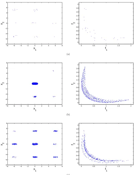
Fig. 4 shows some numerical results of MOP (30) where we have chosenǫ= (0.15,0.15), ∆ = 0.01, and Q= [−20,20]2, i.e., PQ,ǫ consists of a superset of these nine local sets. The figure shows a comparison of a random search algorithm (i.e., a random search generator has been chosen forGenerate() in Algorithm 1), PQ,ǫ-NSGA-II and PQ,ǫ-MOEA (using an initial population of 200 elements and pc = 0.6). For all algorithms, a budget of 5000 function evaluations has been given. It can be observed that the random search generator detects all nine sets, but the approximation of these sets is not sufficient (due to the lack of a local search procedure). PQ,ǫ−N SGA−IIperforms ‘greedy’, i.e., concentrates the search aroundP0,0and nearly

neglects the other sets. The best approximation for this example is given by the result ofPQ,ǫ-MOEA, which yields an approximation of all the nine sets.

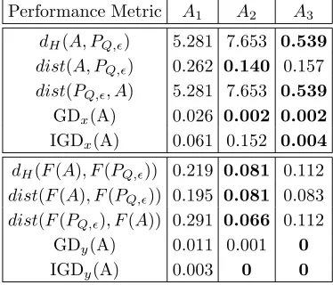
Tables 1 and 2 show the values of the performance metrics proposed in Section 3.2. Table 1 contains the performance metrics which use an expression of PQ,ǫ (we have used a fine discretization in this case) and underline the impression obtained by Fig. 4. PQ,ǫ-NSGA-II yields (as its base algorithm NSGA-II) excellent values for the convergence toward the set of interest (i.e.,dist(A2, PQ,ǫ) and GDx(A2)), and since the image

of the neigborhood ofP0,0 already formsF(PQ,ǫ), also excellent values for the convergence in image space. On the other side, sincePQ,ǫ-NSGA-II does, due to its selection mechanism, not have an evolution pressure toward the regions around the locally optimal sets (32), the values which measure the spread along PQ,ǫ (i.e.,dist(PQ,ǫ, A2) and IGDx(A2)) can not compete with the ones ofPQ,ǫ-MOEA.

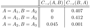
The results obtained by the set coverage metric in Table 2, however, are not that conclusive since only the performance in image space is considered which is not sufficient in this case. The only conclusion which can be drawn from these values is that the random search procedure is outperformed by both evolutionary strategies.

Table 1. Different performance metrics applied on the numerical results of the random search (A1), PQ,ǫ-NSGA-II

(A2), andPQ,ǫ-MOEA (A3) of MOP (30). The results are averaged over 30 test runs.

Performance Metric A1 A2 A3

dH(A, PQ,ǫ) 5.281 7.653 0.539 dist(A, PQ,ǫ) 0.262 0.140 0.157 dist(PQ,ǫ, A) 5.281 7.653 0.539

GDx(A) 0.026 0.002 0.002

IGDx(A) 0.061 0.152 0.004

dH(F(A), F(PQ,ǫ)) 0.219 0.081 0.112 dist(F(A), F(PQ,ǫ)) 0.195 0.081 0.083 dist(F(PQ,ǫ), F(A)) 0.291 0.066 0.112

GDy(A) 0.011 0.001 0

−8 −6 −4 −2 0 2 4 6 8 −8 −6 −4 −2 0 2 4 6 8 x 1 x 2

0 0.5 1 1.5 2

0 0.2 0.4 0.6 0.8 1 1.2 1.4 1.6 1.8 2 f 1 f 2 (a)

−8 −6 −4 −2 0 2 4 6 8

−8 −6 −4 −2 0 2 4 6 8 x 1 x 2

0 0.5 1 1.5 2

0 0.2 0.4 0.6 0.8 1 1.2 1.4 1.6 1.8 2 f 1 f 2 (b)

−8 −6 −4 −2 0 2 4 6 8

−8 −6 −4 −2 0 2 4 6 8 x 1 x 2

0 0.5 1 1.5 2

0 0.2 0.4 0.6 0.8 1 1.2 1.4 1.6 1.8 2 f 1 f 2 (c)

Figure 4. Numerical results for MOP (30) for (a) Random Search, (b)PQ,ǫ-NSGA-II, and (c)PQ,ǫ-MOEA, in parameter

Table 2. Set coverage metric for the numerical results of the three algorithms (Aias in Table 1), averaged over 30 test

runs.

C−ǫ(A, B) C−ǫ(B, A)

A=A1, B=A2 0 0.407

A=A1, B=A3 0 0.412

A=A2, B=A3 0.045 0.001

IV.B. Two Impulse Transfer to Asteroid Apophis

For the bi-impulse problem we analyze an apparently simple case: the direct transfer from the Earth to the asteroid Apophis. The contour lines of the sum of the two ∆v’s is represented in Fig.5a) for t0 ∈

[3675,10500]T _{MJD2000 andT ∈[50,900]days. The intervals for t}

0andT were chosen in such a way that a

wide range of launch opportunities are included.

As can be seen in the specified solution space there is a large number of local minima. Each minimum has a different value but some of them are nested, very close to each other with similar values. For each local minimum, there can be a different front of locally Pareto optimal solutions. The global Pareto front should contain the best transfer with minimum total ∆v and the fastest transfer with minimumT.

The best known approximation of the global Pareto front is represented in Fig. 5b) and was obtained with an extension to MOO problems of the algorithm described by Vasile & Locatelli.22, 23 _{It is a disjoint}

front corresponding to two basins of attraction of two minima as can be seen in Fig. 5a). The lower front is made of solutions with a very low transfer time. The upper front, instead, is made of solutions with a much longer transfer time but a total ∆v similar to the one of the solutions belonging to the lower front.

Besides containing local minima with similar ∆v, the two basins of attraction present similar values of the first objective function. Converging to the upper front is therefore quite a challenge since the lower front has a significantly lower value of the second objective function. It is only when the optimizer converges to a vicinity of the local minimum of the upper front that the latter becomes not dominated by the lower front. The upper front contains the global minimum with a total ∆v = 4.3786 k/s while the lower front contains only a local minimum. It should be noted that, though the front in Fig. 5b) is the global one, it represents only two launch opportunities. Furthermore, for each launch opportunity we would need to characterize the space around each Pareto optimal point.

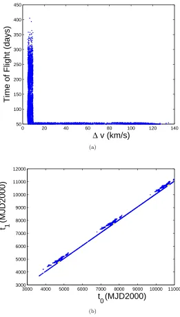
Fig. 6 shows a result for PQ,ǫ-MOEA and using ǫ= (5,5). Since apparently the transfer of 50 days can be reached from any starting date, the bi-objective problem shrinks in practice down to a mono-objective problem with optimal image value aroundy0= (5,50). A search withinN(y0, ǫ, A) revealed different possible

starting times which fall into three clusters: the preimages ofN(y0, ǫ, A) are all located around the points

c1 = (4700,50),c2= (7700,50), andc3= (10700,50). That is, the starting time t0 differs by 3000 days for

neighboring solutions, and by 6000 days in total.

Note that, compared to the accurate solution of the global Pareto front, the extendedǫ−pareto set offers, as required, not only more launch opportunities but also the whole neighboring solutions for each one of them.

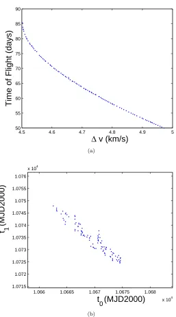
As a comparison we have used the classical NSGA-II to attack the problem (see Fig. 7, note the different scale of these figures to Fig. 6). As anticipated, NSGA-II computes a good approximation of the (very narrow) Pareto set, but in fact generates points only around c3, the maximal difference according to t0 is

given by 35 days.

IV.C. Sequence EVMe

For the MLTGA problem we first consider a relatively simple but significant case: the sequence Earth – Venus – Mercury (EVMe).

For such a mission we have chosen to allow a deterioration of 5% of the mass fraction and of 20 days of the transfer time, compared to an optimal trajectory, which leads to ǫ = (0.05,20). A solution vector for EVMe is given by

y= [t0, t1−t0, k2,1, n1, t2−t1, k2,2, n2]T (33)

where

Departure Time t

0 [MJD2000]

TOF [day]

4000 5000 6000 7000 8000 9000 10000 100

200 300 400 500 600 700 800 900

5 10 15 20

Upper Front

Lower Front

4.2 4.3 4.4 4.5 4.6 4.7 4.8 4.9 5

50 100 150 200 250 300 350

Total ∆ v [km/s]

TOF [day]

Upper Front

Lower Front

Figure 5. a) Earth-Apophis search space, b) Pareto front

and where the numbers of revolutions are fixed ton1= 1 and n2= 7, and choosing rmin,1= 6350, and

rmin,2= 1700.

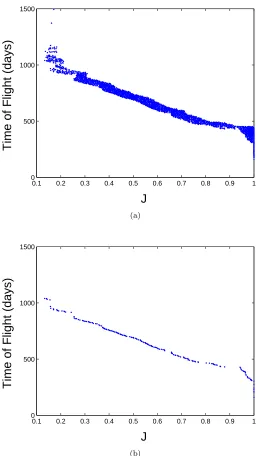
Fig. 8 shows a numerical result ofPQ,ǫ-MOEA, where we have taken an initial population consisting of 200 randomly chosen elements from the domainQ=T ×K2⊂R

5_,p

c= 0.6, ∆ = ∆∗ =ǫ/3, and a budget of 50,000 function calls which took several minutes on an Intel Xeon 3.2 Ghz processor.

Interesting for every non-dominated pointx0 withF(x0) =y0of an archiveAis the set

N(y0, ǫ, A) :={a∈A : F(a)∈B(y0, ǫ)}, (35)

whereB(y, ǫ) :={x∈R

k _{: |x}

i−yi| ≤ǫi, i= 1, .., k}, i.e., the set of solutions inAthose images are close to y0. Since in this design problem the starting datet0 of the transfer is of particular interest one can e.g.

distinguish the entries inN(y0, ǫ, A) by the value oft0. For instance, the final archive displayed in Fig. 8

(a) consists of 2305 solutions whereof 344 are non-dominated. The maximal difference of the value oft0 for

a pointy0 insideN(y0, ǫ, A) is 461 days, and for 43 solutions this maximal difference is larger than one year

(including also values ∆t0 of several days or months which can be also highly interesting for the decision

0 20 40 60 80 100 120 140 50

100 150 200 250 300 350 400 450

∆

v (km/s)

Time of Flight (days)

(a)

3000 4000 5000 6000 7000 8000 9000 10000 11000 3000

4000 5000 6000 7000 8000 9000 10000 11000 12000

t (MJD2000)

t (MJD2000)

(b)

4.5 4.6 4.7 4.8 4.9 5 50

55 60 65 70 75 80 85 90

∆

v (km/s)

Time of Flight (days)

(a)

1.066 1.0665 1.067 1.0675 1.068

x 104 1.0715

1.072 1.0725 1.073 1.0735 1.074 1.0745 1.075 1.0755 1.076

x 104

t (MJD2000)

t (MJD2000)

(b)

sufficient to present the non-dominated front as in the classical multi-objective case. When the DM selects one solutiony0 the setN(y0, ǫ, A) can be displayed, ordered by the value oft0(see Fig. 8 (b)).

0.1 0.2 0.3 0.4 0.5 0.6 0.7 0.8 0.9 1 0

500 1000 1500

J

Time of Flight (days)

(a)

0.1 0.2 0.3 0.4 0.5 0.6 0.7 0.8 0.9 1 0

500 1000 1500

J

Time of Flight (days)

(b)

Figure 8. Numerical result for sequence EVMe. At the top (a), we show the final archive (i.e., theǫ-efficient front) and at the bottom (b) we show the set of non-dominated solutions which is, in this case, sufficient to display for the decision making process.

IV.D. Sequence EVEJ

Finally, we consider the more complex sequence Earth – Venus – Earth – Jupiter (EVEJ) which involves seven free parameters (analog to (33)).

This design problem—as well as other problems of this kind—is characterized by a disconnected feasible domain, and the fraction of this set compared to the entire search space is tiny. In order to increase the performance of the search procedure, we followed24_{and have applied a space pruning algorithm on the search}

(population size 200, budget of 2000 function calls) and have merged the results afterwards. We have chosen again ǫ = (0.05,20), but ∆ = (0,0) since the feasible solutions are not too easy to find, and thus, every promising solution should be captured. Fig. 9 shows one numerical result, which has been obtained within one hour of computational time.

As an example of the use of the result, we assume that the pointy0 has been selected by the DM (see

Fig. 9). The set N(y0, ǫ, Af inal) consists in this case of three solutions with starting times t0,1 = 5085,

t0,2 = 5562, and t0,3 = 6792. Assuming that the values of y0 have been chosen for the transfer and the

archiveA is the basis for the DM, then there are three possibilities: to launch the spacecraft in December 2013 (i.e., 5085 days after 01.01.2000), to launch it 16 months later, or to wait another 3.5 years aftert0,2.

Similar statements hold in this example for all 15 non-dominated solutions xwith J =f1(x)≥0.45, and

thus, also in this case the DM’s decision space has been augmented by allowing approximate solutions.

0.4 0.5 0.6 0.7 0.8 0.9 1

1400 1600 1800 2000 2200 2400 2600

J

Time of Flight (days)

y

Figure 9. Numerical result for sequence EVEJ usingPQ,ǫ-NSGA-II.

V.

Conclusion and Future Work

In this paper, we have considered multi-objective space mission design problems with a novel prospective. For this kind of problems, it is desirable to identify not only the global Pareto set, but also a number of neighboring solutions as well as approximate solutions (which do not have to be in the neighborhood of an optimal solution). In particular, it was shown that each part of the Pareto set can belong to a different launch opportunity. In order to increase the reliability of the mission design, it is required to have a wide launch window for each launch opportunity (i.e. a large number of neighboring solutions with similar cost) and one or more back-up launch opportunities (i.e. one or more nearly optimal sets).

In order to address this problem, we have proposed a new evolutionary strategy which aims for an approximation ofPQ,ǫ, i.e. the solutions which are optimal up to a given (small) value ofǫ. As an example of its effectiveness, we have considered three design problems. The results indicate that the novel approach accomplishes its task within reasonable time and that the idea to include approximate solutions is indeed beneficial since in all cases the decision maker was offered with an enlarged set of useful solutions.

Acknowledgements

The first author acknowledges support from CONACyT project no. 128554. The third author acknowl-edges support from CONACyT project no. 103507.

References

1

R. H. Battin.An Introduction to the Mathematics and Methods of Astrodynamics. AIAA Press, 1999.

2

C. A. Coello Coello, G. B. Lamont, and D. A. Van Veldhuizen. Evolutionary Algorithms for Solving Multi-Objective Problems. Springer, New York, second edition, September 2007. ISBN 978-0-387-33254-3.

3

V. Coverstone-Caroll, J.W. Hartmann, and W.M. Mason. Optimal multi-objective low-thrust spacecraft trajectories.

Computer Methods in Applied Mechanics and Engineering, 186:387–402, 2000.

4

K. Deb, A. Pratap S. Agarwal, and T. Meyarivan. A Fast and Elitist Multiobjective Genetic Algorithm: NSGA–II.IEEE Transactions on Evolutionary Computation, 6(2):182–197, 2002.

5

K. Deb and R. B. Agrawal. Simulated Binary Crossover for Continuous Search Space. Complex Systems, 9:115–148, 1995.

6

K. Deb, M. Mohan, and S. Mishra. Evaluating theǫ-dominated based multi-objective evolutionary algorithm for a quick computation of Pareto-optimal solutions. Evolutionary Computation, 13(4):501–525, 2005.

7

Kalyanmoy Deb and David E. Goldberg. An Investigation of Niche and Species Formation in Genetic Function Opti-mization. In J. David Schaffer, editor,Proceedings of the Third International Conference on Genetic Algorithms, pages 42–50, San Mateo, California, June 1989. George Mason University, Morgan Kaufmann Publishers.

8

David E. Goldberg and Jon Richardson. Genetic algorithm with sharing for multimodal function optimization. In John J. Grefenstette, editor,Genetic Algorithms and Their Applications: Proceedings of the Second International Conference on Genetic Algorithms, pages 41–49, Hillsdale, New Jersey, 1987. Lawrence Erlbaum.

9

T. Hanne. On the convergence of multiobjective evolutionary algorithms. European Journal Of Operational Research, 117(3):553–564, 1999.

10

D. Izzo. Lambert’s problem for exponential sinusoids. Technical report, ACT/ESTEC internal report, April 2005.

11

Joshua Knowles and David Corne. Bounded Pareto Archiving: Theory and Practice. In Xavier Gandibleux, Marc Sevaux, Kenneth S¨orensen, and Vincent T’kindt, editors, Metaheuristics for Multiobjective Optimisation, pages 39–64, Berlin, 2004. Springer. Lecture Notes in Economics and Mathematical Systems Vol. 535.

12

M. Laumanns, L. Thiele, K. Deb, and E. Zitzler. Combining convergence and diversity in evolutionary multiobjective optimization. Evolutionary Computation, 10(3):263–282, 2002.

13

P. Loridan. ǫ-solutions in vector minimization problems. Journal of Optimization, Theory and Application, 42:265–276, 1984.

14

Vilfredo Pareto. Manual of Political Economy. The MacMillan Press, 1971 (original edition in French in 1927).

15

A.E. Petropoulos, J.M. Longuski, and N.X. Vinh. Shape-based analytical representations of low-thrust trajectories for gravity-assist applications. InAAS/AIAA Astrodynamics Specialists Conference, AAS Paper 99-337, Girdwood, Alaska, 1999.

16

G. Rudolph and A. Agapie. Convergence properties of some multi-objective evolutionary algorithms. InProceedings of the 2000 Conference on Evolutionary Computation, volume 2, pages 1010–1016, 2000.

17

G¨unter Rudolph, Boris Naujoks, and Mike Preuss. Capabilities of EMOA to Detect and Preserve Equivalent Pareto Subsets. In Shigeru Obayashi, Kalyanmoy Deb, Carlo Poloni, Tomoyuki Hiroyasu, and Tadahiko Murata, editors,Evolutionary Multi-Criterion Optimization, 4th International Conference, EMO 2007, pages 36–50, Matshushima, Japan, March 2007. Springer. Lecture Notes in Computer Science Vol. 4403.

18

Oliver Sch¨utze, Carlos A. Coello Coello, and El-Ghazali Talbi. Approximating theǫ-efficient set of an MOP with stochastic search algorithms. In A. Gelbukh and A. F. Kuri Morales, editors,Mexican International Conference on Artificial Intelligence (MICAI-2007), pages 128–138. Springer-Verlag Berlin Heidelberg, 2007.

19

Oliver Sch¨utze, Carlos A. Coello Coello, Emilia Tantar, and El-Ghazali Talbi. Computing finite size representations of the set of approximate solutions of an mop with stochastic search algorithms. InGECCO ’08: Proceedings of the 10th annual conference on Genetic and evolutionary computation, pages 713–720, New York, NY, USA, 2008. ACM.

20

Oliver Sch¨utze, Massimiliano Vasile, and Carlos A. Coello Coello. Approximate solutions in space mission design. In

PPSN ’08: Proceedings of the 10th International Conference on Parallel Problem Solving From Nature, pages 805–814, 2008.

21

Oliver Sch¨utze, Massimiliano Vasile, Oliver Junge, Michael Dellnitz, and Dario Izzo. Designing optimal low-thrust gravity-assist trajectories using space pruning and a multi-objective approach.Engineering Optimization, 41(2):155–181, February 2009.

22

M. Vasile. Hybrid behavioural-based multiobjective space trajectory optimization. In Chi-Keong Goh, Yew-Soon Ong, and Kay Chen Tan, editors,Multi-Objective Memetic Algorithms, volume 171 ofStudies in Computational Intelligence, pages 231–253. Springer, 2009.

23

M. Vasile and M. Locatelli. A hybrid multiagent approach for global trajectory optimization. Journal of Global Opti-mization, 44(4):461–479, August 2009.

24

M. Vasile, O. Sch¨utze, O. Junge, G. Radice, and M. Dellnitz. Spiral trajectories in global optimisation of interplanetary and orbital transfers. Ariadna study report ao4919 05/4106, contract number 19699/nl/he, European Space Agency, 2006.

25

D. A. Van Veldhuizen. Multiobjective Evolutionary Algorithms: Classifications, Analyses, and New Innovations. PhD thesis, Department of Electrical and Computer Engineering. Graduate School of Engineering. Air Force Institute of Technology, Wright-Patterson AFB, Ohio, May 1999.

26

27