A course space construction based on local Dirichlet-to-Neumann maps

A COARSE SPACE CONSTRUCTION BASED ON LOCAL DIRICHLET-TO-NEUMANN MAPS∗

FR ´ED ´ERIC NATAF†, HUA XIANG‡, VICTORITA DOLEAN§,AND NICOLE SPILLANE†

Abstract. Coarse-grid correction is a key ingredient of scalable domain decomposition methods. In this work we construct coarse-grid space using the low-frequency modes of the subdomain Dirichlet-to-Neumann maps and apply the obtained two-level preconditioners to the extended or the original linear system arising from an overlapping domain decomposition. Our method is suitable for parallel implementation, and its efficiency is demonstrated by numerical examples on problems with large heterogeneities for both manual and automatic partitionings.

Key words. domain decomposition, coarse grid, deflation, heterogeneous coefficients

AMS subject classifications.65N55, 65F10, 65N30

DOI.10.1137/100796376

Notation.

A coefficient matrix of the linear system_Ax=_b

M preconditioner for_A

Z, Y full rank matrices which span the coarse-grid subspaces

E E=_YT_{AZ, Galerkin matrix or coarse-grid matrix}

Ξ Ξ =_ZE−1_YT_{, coarse-grid correction matrix in multigrid and}

do-main decomposition methods

PD PD=I−AΞ =I−AZ(YTAZ)−1YT

QD QD=I−ΞA=I−Z(YTAZ)−1YTA

PBN N PBN N =QDM−1PD+ZE−1YT

PADEF2 PADEF2=QDM−1+ZE−1ZT

1. Introduction. We consider the solution of the linear system _Ax= _b ∈ Rp

arising from the discretization of an elliptic boundary value problem (BVP) of the type

(1.1) ηu−div(κ∇u) =f in Ω,

B(_u) = 0 on_∂Ω_,

where Ω is a bounded domain ofRd(_d= 2 or 3),_Bis a suitable boundary condition,_κ is a positive diffusion function which can be discontinuous, and_η≥0. When using an iterative method in a one-level domain decomposition framework, one may encounter a long stagnation or a slow convergence, especially when the number of subdomains is

∗_{Submitted to the journal’s Methods and Algorithms for Scientific Computing section May 25,}

2010; accepted for publication (in revised form) April 26, 2011; published electronically July 21, 2011. The first and second authors acknowledge the support of the French National Research Agency (ANR PETAL) and CNRS via the GDR MOMAS.

http://www.siam.org/journals/sisc/33-4/79637.html

†_{Laboratoire J.L. Lions, CNRS UMR 7598, Universit´e Pierre et Marie Curie, Paris 75005, France}

([email protected], [email protected]).

‡_{School of Mathematics and Statistics, Wuhan University, Wuhan 430072, P. R. China (xiang@}

ann.jussieu.fr).

§_{Laboratoire J.-A. Dieudonn´e, CNRS UMR 6621, Universit´e de Nice-Sophia Antipolis, Parc}

Val-rose, 06108 Nice Cedex 02, France ([email protected]).

1623

large. Even when_κ≡1, the convergence of a one-level domain decomposition method (DDM) presents a long plateau of stagnation. Its length is related to the number of subdomains of the decomposition in one direction. For example, we know that for the problem divided into_N subdomains in a one-way partitioning, convergence can never be achieved in less than_N −1 iterations since the exchange of information between the subdomains is reduced to their common interfaces. Thus, the global information transfers from one subdomain only to its neighbors [13, 16]. One needs a two-level method to have a scalable algorithm, i.e., an algorithm whose convergence rate is weakly dependent on the number of subdomains; see [26] and references therein.

Two-level domain decomposition methods are closely related to multigrid (MG) methods and deflation corrections; see [24] and references therein. These methods are defined by two ingredients: a full rank matrix_Z∈Rp×m_{withmpand an algebraic}

formulation of the correction. These techniques imply solving a reduced-size problem of order_m×_m, called a coarse-grid problem. The space spanned by the columns of

Z should ideally contain the vectors responsible for the stagnation of the one-level method. We will come back later to the choice of_Z in the framework of DDMs and focus for now on the various algebraic ways to improve convergence by using a coarse grid.

According to [24], for a DDM, a well-known coarse-grid correction preconditioner is of the form_I+_ZE−1_ZT_{, whereE=Z}T_{AZ is the coarse-grid matrix used to speed}

up convergence. The abstract additive coarse-grid correction proposed in [18] is_M−1+

ZE−1ZT, where_M−1 is the additive Schwarz preconditioner, a sum of local solvers in each subdomain, which can be implemented in parallel. The first term is a fine grid solver, and the second term represents a coarse solver. Hence it is called the two-level additive Schwarz preconditioner. The BPS preconditioner introduced by Bramble, Pasciak, and Schatz [1] is of this type. In the context of DDMs, we mention the balancing Neumann–Neumann preconditioner and the FETI (finite element tearing interconnection) algorithm, which have been extensively investigated; see [26] and references therein. For symmetric systems the balancing preconditioner was proposed by Mandel [14]. The abstract balancing preconditioner [14] for nonsymmetric systems reads [8]

(1.2) _{PBN N}=_QDM−1_PD+_ZE−1_YT_.

For the preconditioner _{PBN N}, if we choose the initial approximation_x0 = Ξ_b, then the action of_PD is not required in practice; see [26, p. 48]. Note that the MG V(1,1)-cycle preconditioner_PMG is closely related to_{PBN N}. Choosing the proper smoother

M in _{PBN N}, we can ensure that _PMG and _{PBN N} are symmetric positive definite (SPD), and_PMGAand_{PBN NA}have the same spectrum [25].

For an SPD system, by choosing_Y =_Z, the authors in [24] define

(1.3) _PADEF2=_QDM−1+_ZE−1_ZT_,

which is as robust as _{PBN N} but usually less expensive [24]. The two-level hybrid Schwarz preconditioner in [23, p. 48] has the same form as_PADEF2. It is shown in [24] that with a proper choice of the starting vector the preconditioners_PADEF2and

PBN N are equivalent.

Given the coarse-grid subspace, we can construct the two-level preconditoners above. An effective two-level preconditioner is highly dependent on the choice of the coarse-grid subspace. We will now focus on the choice of the coarse space _Z in the context of DDMs for problems of type (1.1) with heterogeneous coefficients. In this case, the coarse space is made of vectors with support in one subdomain

or one subdomain and its neighbors. When the jumps in the coefficients are inside the subdomains (and not on the interface) or across the interface separating the subregions, the use of a fixed number of vectors per subdomain in _Z gives good results; see [6, 15, 19, 20, 4, 5]. When the discontinuities are along the interfaces between the subdomains, results are not so good.

Here, we propose constructing a coarse subspace such that the two-level method is robust with respect to heterogeneous coefficients for an arbitrary domain decom-position. Even if the discontinuities are along the interface, as in the case with lay-ered coefficients and a one-way decomposition in the orthogonal direction (see section 4.1), the iteration counts are very stable with respect to jumps of the coefficients. Our method is based on the low-frequency modes associated with the Dirichlet-to-Neumann (DtN) map on each subdomain. After obtaining the eigenvectors associated with the small eigenvalues of DtN, we use the harmonic extension to the whole sub-domain. It is efficient even for problems with large discontinuities in the coefficients. Moreover, it is suitable for parallel implementation. We apply such a two-level pre-conditioner to the original linear system (2.1) and to the extended one (2.2) arising from the DDM.

The paper is organized as follows. In section 2, we introduce the two-level precon-ditioners: the additive Schwarz (AS), the restricted additive Schwarz (RAS), and the Jacobi–Schwarz (JS) with the coarse-grid correction. The construction of coarse-grid spaces is presented in section 3. In section 4, numerical tests on the model prob-lem demonstrate the efficiency of our method. Some concluding remarks are given in section 5.

2. Algebraic DDMs. Without loss of generality, we consider here a decompo-sition of a domain Ω into two overlapping subdomains Ω₁ and Ω₂. The overlap is denoted by_O:= Ω₁∩Ω₂. This yields a partition of the domain: ¯Ω = ¯Ω(1)_I ∪_O¯∪Ω¯(2)_I , where Ω(_Ii):= Ω_i\_O¯,_i= 1_,2. At the algebraic level this corresponds to a partition of

the set of indicesN into three sets: N_I(1),N_O, andN_I(2); see Figure 2.1.

After the discretization of the BVP (1.1) defined in domain Ω, we obtain a linear system of the following form:

A u:= ⎡ ⎢ ⎢ ⎣

A(1)_II A(1)_IO A(1)_OI AOO A(2)OI

A(2)_IO A(2)_II

⎤ ⎥ ⎥ ⎦ ⎡ ⎢ ⎣u

(1)

I

uO

u(2)I

⎤ ⎥ ⎦=

⎡ ⎢ ⎣f

(1)

I

fO

fI(2)

⎤ ⎥ ⎦.

(2.1)

u

O

u

O (1)

u

O (2)

u

I

(1)

_u

I (2)

Ω₁

Ω₂

Fig. 2.1_{.Decomposition into two overlapping subdomains.}

We can also define the extended linear system by considering twice the variables located in the overlapping region,

˜

A _u˜:= ⎡ ⎢ ⎢ ⎢ ⎢ ⎣

A(1)II A

(1)

IO

A(1)OI AOO A(2)OI

A(1)_OI AOO A(2)_OI

A(2)_IO A(2)_II

⎤ ⎥ ⎥ ⎥ ⎥ ⎦ ⎡ ⎢ ⎢ ⎢ ⎣

u(1)I

u(1)O

u(2)O

u(2)I

⎤ ⎥ ⎥ ⎥ ⎦= ⎡ ⎢ ⎢ ⎣

f_I(1) fO

fO

fI(2)

⎤ ⎥ ⎥ ⎦,

(2.2)

where the subscript “_O” stands for “overlap,”_u(_Oi)are the duplicated variables in the

overlapping domain_O, and_u(_Ii)are variables in the subdomain Ωi_I. It is easy to check that if_AOO is invertible, there is an equivalence between problems (2.1) and (2.2).

Classical preconditioners for problem (2.1) are the AS and the RAS methods; see [2] or [26] and references therein. Let _Rj be the rectangular restriction matrix to subdomain Ω_j, _j = 1_,2. Let _Dj,_j = 1_,2, be diagonal matrices which correspond to a partition of unity in the sense that

RT1D1R1+_RT_2D2R2=_{I .}

By defining ˜_Rj :=_DjRj, we have

˜

RT1R1+ ˜RT2R2=I .

Then the AS preconditioner reads

(2.3) _MAS−1:=_RT_1A−₁1_R1+_RT_2A−₂1_R2,

and the RAS method reads

(2.4) _un+1=_un+ ( ˜_RT_1A−₁1_R1+ ˜_RT_2A−₂1_R2)(_f−_Aun)_,

where _Ai := _RiART

i , i = 1,2. From the iterative scheme (2.4), we can define the

preconditioner

M_RAS−1 := ˜_R1T_A−₁1_R1+ ˜_RT_2A−₂1_R2.

Note that the RAS preconditioner is nonsymmetric. It leads to an iterative method that is identical to the discretization of the continuous JS method; see [7].

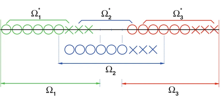
An illustration of the RAS method is given in Figure 2.2 for a three-subdomain decomposition, where Ω_iare overlapping subdomains and Ω∗_i are nonoverlapping sub-domains. If we take_Dito have zero entries for nodes in the region Ω_i\Ω∗_i, we define

˜

RT1 = ⎡ ⎣IΩ∗1

0 0

⎤

⎦_{, R}˜T

2 =

⎡ ⎣_IΩ0∗

2 0

⎤

⎦_{, R}˜T

3 =

⎡ ⎣ 00

IΩ∗ 3 ⎤ ⎦_,

R1=IΩ1 0 0 _{, R2}=0 _IΩ2 0 _{, R3}=0 0 _{IΩ3 ,}

where_IΩi is the identity matrix whose dimension equals the number of unknowns in Ω_i.

Ω

Ω

*

Ω

*

Ω

Ω

Ω

Fig. 2.2_{.RAS (ndomain= 3,noverlap= 4}−_{1,nxpt= 6; see section4.1for these parameters).}

The circles and crosses stand for the unknowns in each subdomain.

For our extended linear system (2.2), a natural preconditioner can be built by using its diagonal blocks. For the two-subdomain case (2.2), the block diagonal pre-conditioner_MJS is

MJS:=

⎡ ⎢ ⎢ ⎢ ⎢ ⎣

A(1)II A

(1)

IO

A(1)OI AOO

AOO A(2)OI

A(2)_IO A(2)_II

⎤ ⎥ ⎥ ⎥ ⎥ ⎦, (2.5)

and one can easily notice that_MJS−1can be computed in parallel. The resulting method will be referred to as the JS method. When used in a Richardson algorithm such as in (2.4), it was proved in [3] that_MJS applied to (2.2) and_MRAS applied to (2.1) lead to equivalent algorithms. But, as we shall see from numerical experiments, two-level methods applied to (2.2) or to (2.1) are not necessarily equivalent.

Note that even though the original matrix_A is symmetric, the extended one ˜_A is not. As for the preconditioners,_MAS and _MJS are symmetric but_MRAS is not. As a result, the only case where we have both a symmetric matrix and a symmetric preconditioner is when_MAS applies to the original matrix_A. In this case, the Krylov method that we use is the CG algorithm. In the other two cases (namely,_MJSapplied to the extended matrix and _MRAS applied to the original system), we use GMRES [22].

Using preconditioners_MAS,_MJS, or_MRAS, we can remove the influence of very large eigenvalues of the coefficient matrix, which correspond to high-frequency modes. But the small eigenvalues still exist and hamper the convergence. These small eigen-values correspond to low-frequency modes and represent certain global information. We need a suitable coarse-grid space to efficiently deal with them.

3. The coarse-grid space construction. A key problem is the choice of the coarse subspace. Ideally, we can choose the deflation subspace _Z which consists of the eigenvectors associated with the small eigenvalues of the preconditioned operator. But the lower part of the spectrum of a matrix is costly to obtain. The cost is in any case larger than the cost of solving a linear system. Thus, there is a need to

choose the coarse space a priori. For instance, in [17], Nicolaides defines the deflation subspace_Z as

(_zj)_i=

1 if_i∈Ω∗_j, 0 otherwise_,

whose matrix form is

(3.1) _Z =

⎡

⎣1Ω∗1 0 0 0 1_Ω∗

2 0

0 0 1_Ω∗ 3 ⎤ ⎦_,

where 1_Ω∗

i is a vector of all ones, and its length equals the number of unknowns in

Ω∗_i. Recall that the subdomains Ω∗_i are nonoverlapping as shown in Figure 2.2. In [27, 28], the projection vectors_zi are chosen in a similar but more complicated way. Definition (3.1) is also used as the aggregation-based coarse level operator in [9]. Originally (3.1) was used for disjoint sets but not for the overlapping case. In the following, we use it in the overlapping case as well. This coarse space performs well in the constant coefficient case. But when there are jumps in the coefficients, it cannot prevent stagnation in the convergence.

We now propose a construction of the coarse space that will be suitable for parallel implementation and efficient for accelerating the convergence for problems with highly heterogeneous coefficients and arbitrary domain decompositions. For both the original system (2.1) and the extended one (2.2), we still choose_Z such that it has the form

(3.2) _Z=

⎡ ⎢ ⎢ ⎢ ⎢ ⎣

W1 0 · · · 0

..

. _W2 · · · 0 ..

. ... · · · ...

0 0 · · · _WN

⎤ ⎥ ⎥ ⎥ ⎥ ⎦,

where_N is the number of overlapping subdomains. However,_Wi _{is now a}

rectangu-lar matrix whose columns are based on the harmonic extensions of the eigenvectors corresponding to small eigenvalues of the DtN map in each subdomain Ω_i. Note that the sparsity of the coarse operator_E =_ZT_{AZ is a result of the sparsity of Z. The}

nonzero components of_E correspond to adjacent subdomains.

More precisely, let us consider first at the continuous level the DtN map DtN_Ωi. Let_u: Γ_i →R,

DtN_Ωi(_u) =_κ∂v

∂ni

Γi

,

where_v satisfies

(3.3)

L(_v) := (_η−div(_κ∇))_v= 0 in Ω_i,

v=_u on Γ_i,

and Γ_i is the interface boundary. If the subdomain is not a floating one (i.e., _∂Ω_i∩

∂Ω = ∅), we use on the part of the global boundary the boundary condition from the original problem _B(_u) = 0. To construct the coarse-grid subspace, we use the low-frequency modes associated with the DtN operator:

(3.4) DtN_Ωi(_u) =_{λκ u}

Ωi Ωi+1

Ωi−1 _en

i

en+1

i−1 en+1i+1

Ωi Ωi+1

Ωi−1 _en

i

en+1

i−1 _en+1_i+1

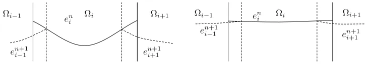
Fig. 3.1_{.Fast (left) or slow (right) convergence of the Schwarz algorithm.}

with

(3.5) _{λ <}1_/diam(Ω_i)_,

where_diam(Ω_i) is the diameter of subdomain Ω_i.

We first motivate our choice of a coarse space based on the DtN map. We write the original Schwarz method at the continuous level, where the domain Ω is decomposed in a one-way partitioning. The error_en

i between the current iterate at stepnof the

algorithm and the solution _u|Ωi (_en

i :=uni −u|Ωi) in subdomain Ωi at step nof the

algorithm satisfies

L(_en_i+1) = 0 in Ω_i,

eni+1=

j=iξijejn on ¯Ωi∩∂Ωj,

where_ξj_i is such that

j=i

ξij= 1∂Ωi.

In the 1D (one-dimensional) example sketched in Figure 3.1, we see that the rate of convergence of the algorithm is related to the decay of the harmonic functions_en_i in the vicinity of_∂Ω_ivia the subdomain boundary condition (BC). Indeed, a small value for this BC leads to a smaller error in the entire subdomain thanks to the maximum principle.

Moreover, a fast decay for this value corresponds to a large eigenvalue of the DtN map, whereas a slow decay corresponds to small eigenvalues of this map because the DtN operator is related to the normal derivative at the interface and the overlap is thin. Thus the small eigenvalues of the DtN map are responsible for the slow convergence of the algorithm, and it is natural to incorporate them in the coarse-grid space.

We now explain why we keep only eigenvectors with eigenvalues smaller than 1_/diam(Ω_i) in the coarse space. We start with the constant coefficient case_κ = 1. In this case, the smallest eigenvalue of the DtN map is zero and corresponds to the constant function 1. For a shape regular subdomain, the first positive eigenvalue is of order 1_/diam(Ω_i); see [10]. Keeping only the constant function 1 in the coarse space leads to good numerical convergence; see Figure 4.2 below. In the case of high contrasts in the coefficient_κ, the smallest eigenvalue of the DtN map is still zero. But due to the variation of the coefficients we may have positive eigenvalues smaller than 1_/diam(Ω_i). In order to have convergence behavior similar to that of the constant coefficient case, it is natural to keep all eigenvectors with eigenvalues smaller than 1_/diam(Ω_i).

To obtain the discrete form of the DtN map, we consider the variational form of

(3.3). Let’s define the bilinear form_ai :_H1(Ω_i)×_H1(Ω_i)→R,

ai(w, v) :=

Ωi

ηwv+_κ∇_w· ∇_v.

With a finite element basis {_φk}, the coefficient matrix of a Neumann BVP in domain Ω_i is

A(_kli)=

Ωi

ηφkφl+κ∇φk· ∇φl.

Let_I (resp., Γ_i) be the set of indices corresponding to the interior (resp., boundary) degrees of freedom, and _nΓi := #(Γ_i) the number of interface degrees of freedom. Note that for the whole domain Ω the coefficient matrix is given by

Akl=

Ωηφkφl

+_κ∇_φk· ∇_φl.

With block notation, we have

A(_IIi)=_{AII, A}(_Γi)

iI =AΓiI, and A_I(i_Γ)_i =AIΓi.

But the matrix _A(_Γi)

iΓi refers to the matrix prior to assembly with the neighboring

subdomains and thus cannot be simply extracted from the coefficient matrix_A. In problem (3.3), we use Dirichlet BCs. Let _U ∈ RnΓ_{i and u :=}

k∈ΓiUkφk. Let

v := _k∈IVkφk+_l∈Γ

iVlφl be the finite element approximation of the solution

of (3.3). Letting_VI = (_Vk)_k∈I, we have with obvious notation

(3.6) _AIIVI+_AIΓiU = 0_.

A variational definition of the flux reads

Γi

κ∂v ∂nφk=

Ωi

ηvφk+κ∇v· ∇φk

for all_φk,_k∈Γ_i. So the variational formulation of the eigenvalue problem (3.4) reads

(3.7)

Ωi

ηvφk+κ∇v· ∇φk =λ

Γi

κv φk

for all_φk,_k∈Γ_i. Let_Mκ,Γi be the weighted mass matrix

(_Mκ,Γi)_kl:=

Γi

κφkφl ∀k, l∈Γi.

The compact form of (3.7) is

A(_Γi_i)_ΓiU +_AΓiIVI =_{λMκ,ΓiU .}

With (3.6), the discrete form of (3.4) is a generalized eigenvalue problem

(3.8) (_A(_Γi)

iΓi−AΓiIA

−1

IIAIΓi)U =λ Mκ,ΓiU .

The step-by-step procedure for constructing the rectangular matrices_Wi_{in the coarse}

space matrix_Z (see (3.2)) is as follows.

Algorithm 1. In parallel for all subdomains1≤i≤N, the following hold:

1. Compute eigenpairs of(3.8),(_Ui

1, λi1),(U2i, λi2), . . . ,(Umii, λimi), such that

λi1≤ · · · ≤λimi <1/diam(Ωi)≤λimi+1≤ · · ·.

2. Compute their harmonic extensions,

Vki:= (−A−II1AIΓiUki, Uki)T, 1≤k≤mi.

3. The final formula for the rectangular matrix_Wi with_mi columns depends on

the system to be solved:

If the extended system is solved (see(2.2)), then

Wi= [_V1i|_{. . .}|_Vmi_i]_.

If the original system is solved (see (2.1)), then

Wi= [_DiV1i|_{. . .}|_DiVmi_i]_.

We call this procedure the_ZD2N method. We also use_ZD2N to denote the coarse-grid space constructed by this method. Its construction is fully parallel. Similarly, we call _{ZN ico} the method of Nicolaides or the corresponding coarse-grid space. Let us remark that when _η = 0 and the subdomain does not touch the boundary of Ω, the lowest eigenvalue of the DtN map is zero, and the corresponding eigenvector is a constant vector. Thus,_{ZN ico} and_ZD2N coincide. As we shall see in the next section, when a subdomain has several jumps of the coefficient, taking_{ZN ico} is not efficient, and it is necessary to take_ZD2N with more than one vector per subdomain.

Note that when we work on the original system, the definition of the coarse space involves a partition of unity via the matrices_Di. Thus the vectors of the coarse space are able to span the zero energy modes of the original problem if there are no Dirichlet BCs. In the following numerical tests, we construct the diagonal matrices_Di in the spirit of the RAS method. Let _fi : Ω_i →Rbe the characteristic function of ¯Ω∗_i. We define _χi(_x) as the P1 finite element interpolation of _fi(_x)_/jfj(_x). Then, we set (withMatlabnotation)D_i:= diag(χ_i).

4. Numerical results. From a practical point of view, it is more difficult to work on the extended system (2.2) than on the original one (2.1). Indeed, when working on (2.2), we have to create extra data structures. For this reason, we first consider in section 4.1 a one-way decomposition of the domain. This enables us to work both on the original system (2.1) and on the extended one (2.2). In section 4.2 an arbitrary decomposition is considered; we will work only on the original system (2.1). In all numerical results, the residual reduction factor to convergence is 10−6.

4.1. One-way domain decomposition. In order to illustrate numerically the behavior of the coarse space, we first consider the following model problem:

Lu:=

− ∂ ∂xc(y)

∂ ∂x−

∂ ∂yd(y)

∂

∂y +η(y)

u(_{x, y}) =_f(_{x, y}) in (0_{, L})×(0_,1)_,

where the length_Lof the domain is proportional to the number of subdomains. We use Neumann BCs on the top and the bottom, a Dirichlet BC on the left, and (_∂/∂n+_α)_u= 0_{, α}1, on the right boundary; see Figure 4.1.

All the test cases are described in Table 4.1. We first consider the constant coefficient case with _c(_y) = _d(_y) = 1_.0 (CONST in Table 4.1). Afterward we will

Ωi

u=

0

∂u/∂n =0

(

∂

/

∂

n+

α

)u

=

0

ΓR ΓL

∂u/∂n =0

δ δ

Fig. 4.1_{.Subdomains and boundary conditions.}

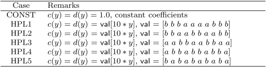
Table 4.1

Test cases: b= 1,a= 100000.

Case Remarks

CONST c(y) =d(y) = 1.0, constant coefficients

HPL1 c(y) =d(y) =val[10∗y],val= [b b b a a a a b b b] HPL2 c(y) =d(y) =val[10∗y],val= [b b a a b b a a b b] HPL3 c(y) =d(y) =val[10∗y],val= [a a b b a a b b a a] HPL4 c(y) =d(y) =val[10∗y],val= [a b b a b b a b b a] HPL5 c(y) =d(y) =val[10∗y],val= [b a b a b a b a b a]

test more difficult cases, with discontinuities in the coefficients, such as_c(_y) =_d(_y) = val[10∗_y], where valis an array that defines the heterogeneity pattern and that depends on two parameters _aand_b (e.g., in the case HPL3, val= [_{a a b b a a b b a}

a] means that there are three high-permeability layers). In our tests we take_a= 105,

b= 1, and_η= 10−7.

In addition, we use the following parameters in our tests:

• ndomainrepresents the number of subdomains.

• noverlap stands for the overlap in thex-direction; correspondingly the width

of the overlap is_δ= (_noverlap+ 1)_h, where_his the mesh size.

• (_nxpt+_noverlap) is the number of grid points in the _x-direction in one

sub-domain.

• nypt is the number of grid points in they-direction.

These numerical tests are performed in Matlab. We compare the two coarse grids,

namely the Nicolaides one (3.1) and the one defined in Algorithm 1 (D2N), only for the RAS and JS preconditioners. See section 4.2 for the RAS and AS methods. We use full GMRES as the linear solver, together with the left preconditioner_PADEF2, which is constructed by taking_Z equal to _{ZN ico} or to _ZD2N, where _ZD2N is of the form (3.2). Please note that when using the left-preconditioned GMRES on_Ax=_b, the residual||_b−_Ax¯||is returned for the approximate solution ¯_x(see Figures 4.2–4.6).

4.1.1. The original vs. extended system. We first compare the effect of the coarse-grid correction when applied to the original system (2.1) (RAS method) or to the extended system (2.2) (JS method). We begin with the Nicolaides coarse-grid space. As expected when there is no coarse-grid correction, RAS and JS perform similarly and have a plateau in the convergence curve.

For the constant case in Figure 4.2, the piecewise coarse-grid space of Nicolaides is quite good for both the extended system and the original system. It works better

0 20 40 60 80 100 120 10−6

10−4 10−2 100 102 104

M_JS P_ADEF2: JS + Z_Nico P_ADEF2: JS + Z_D2N RAS P

ADEF2: RAS + ZNico

P_ADEF2: RAS + Z_D2N

Fig. 4.2. Case CONST for JS and RAS using coarse grids. n_domain = 32, n_overlap = 1,

nxpt= 8,nypt= 16. BothZN ico andZD2N work well for the constant case.

0 50 100 150 200 250 300

10−6 10−4 10−2 100 102 104

M_JS P_ADEF2: JS + Z_Nico P_ADEF2: JS + Z_D2N RAS P

ADEF2: RAS + ZNico

P_ADEF2: RAS + Z_D2N

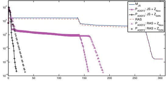
Fig. 4.3.Case HPL2for JS and RAS with coarse-grid correction.n_domain= 64,n_overlap= 1,

nxpt= 8,nypt= 16. ZN ico does not work well, whileZD2N gives fast convergence.

on the extended system (2.2) (JS method) than on the original system (2.1) using RAS (22 versus 36 iterations).

For the case with discontinuities, _{ZN ico} is not good. For this kind of problem,

ZD2N gives a much faster convergence; see Figure 4.3. Note that for the case HPL2,

the number of small eigenvalues determined by (3.5) is 2, which is equal to the number of high-permeability layers; see [27].

We can see that our_ZD2N method works well on both the extended system and the original system, but it gives better convergence on the extended system. It seems to us that this is due to the fact that for JS we do not need a partition of unity. For RAS this partition of unity is necessary for the method to be able to span the zero energy modes of the original problem. But then, the local harmonicity of the coarse space components is lost. This is the reason why we will further investigate our_ZD2N method on the extended system.

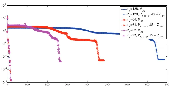
4.1.2. The robustness of the Z_D2N method. In the following we test the robustness of the approach with respect to the various parameters of the problem: jumps of the coefficients, number of subdomains, mesh size, and size of the overlap.

0 100 200 300 400 500 600 700 800 10−6

10−4 10−2 100 102 104 106

n_d=128, M_JS n

d=128, PADEF2: JS + ZD2N

n_d=64, M_JS n_d=64, P_ADEF2: JS + Z_D2N n_d=32, M_JS n

d=32, PADEF2: JS + ZD2N

Fig. 4.4. Case HPL3 with various number of subdomains. n_domain= 128(crosses), 64

(cir-cles),32(triangles),noverlap= 1,nypt= 16. ZD2N: dotted lines,JS: solid lines.

Table 4.2

Case HPL2 with the ZD2N coarse space for jumps in the coefficients ranging from1to 106.

ndomain= 32,noverlap= 3,nxpt= 8,nypt= 16.

Jumps in coefficient 1 10 102 ₁₀3 ₁₀4 ₁₀5 ₁₀6

Iteration counts 15 24 10 10 10 11 11

0 20 40 60 80 100 120 140 160 180 200 220

10−8 10−6 10−4 10−2 100 102 104 106

h=1/64, M_JS h=1/64, P_ADEF2: JS + Z_D2N h=1/32, M

JS

h=1/32, P

ADEF2: JS + ZD2N

h=1/16, M_JS h=1/16, P_ADEF2: JS + Z_D2N

Fig. 4.5_{.Case HPL3with various mesh sizes:1/64(crosses),1/32(circles), and1/16}

(trian-gles);noverlap= 1,ndomain= 16. ZD2N: dotted lines,JS: solid lines.

Figure 4.4 shows that, when we use a coarse space, the iteration numbers are almost constant as the number of subdomains increases. The three convergence curves with_ZD2N are difficult to distinguish.

We also consider the robustness with respect to the size of the jumps. We take as an example in Table 4.2 the case HPL2 with_a ranging from 1 to 106. Using the criterion (3.5), in each subdomain two small eigenvectors are chosen to construct the

ZD2N coarse space. We see that the iteration counts are almost constant as the size

of the jump in the coefficients increases by six orders of magnitude.

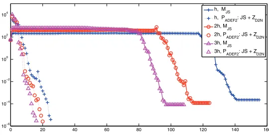
In Figure 4.5, we plot the convergence curves for three successive refinements of the mesh. We see an increase in the number of iterations, which can be related to the

0 20 40 60 80 100 120 140 160 10−6

10−4 10−2 100 102 104

h, M_JS h, P

ADEF2: JS + ZD2N

2h, M_JS 2h, P_ADEF2: JS + Z_D2N 3h, M_JS 3h, P

ADEF2: JS + ZD2N

Fig. 4.6.HPL1with various overlaps: h(crosses),2h(circles), and3h(triangles);n_domain= 32,nxpt=nypt= 16. ZD2N: dotted lines,JS: solid lines.

0 1 2 3 4 5 6 7 8

−4 −2 0 2 4x 10

−14 eig(A)

0 0.2 0.4 0.6 0.8 1 1.2 1.4 1.6 1.8 2

−2 −1 0 1 2x 10

−14 eig(MJS

−1_A)

0 0.2 0.4 0.6 0.8 1 1.2 1.4 1.6 1.8 2

−1 −0.5 0 0.5 1x 10

−11 eig(PADEF2A )

Fig. 4.7_{. Spectra of CONST case. ndomain = 16, noverlap= 1, nxpt = 8,nypt = 16. The}

third row is the result of theZD2N method with one small eigenvector of the DtN map taken into

account in each subdomain.

fact that the convergence rate of the Schwarz method depends on the physical size of the overlap. Here, we have a two element overlap, and thus the physical size of the overlap decreases as the mesh is refined.

In Figure 4.6, we consider the test HPL1 with various sizes of overlap,_h, 2_h, and 3_h, solved with the _ZD2N coarse space or without any coarse space (JS). For both methods, the iteration counts are improved as the overlap is increased. This is in agreement with the theory of the Schwarz method.

From the residual curves, we see that our method is very efficient and robust.

4.1.3. Spectral analysis of the preconditioned system. In Figures 4.7 and 4.8, we display the spectra of the CONST and HPL5 cases, respectively, for the original system, the one-level method, and the two-level method with the D2N coarse grid using _PADEF2. The spectrum of the preconditioned matrices has three characteristics:

• the eigenvalues are between 0 and 2;

• the spectrum is more clustered;

0 1 2 3 4 5 6

x 105

−1 −0.5 0 0.5 1x 10

−9 eig(A)

0 0.2 0.4 0.6 0.8 1 1.2 1.4 1.6 1.8 2

−1 −0.5 0 0.5 1x 10

−15 eig(MJS

−1A)

0 0.2 0.4 0.6 0.8 1 1.2 1.4 1.6 1.8 2

−0.5 0 0.5 1x 10

−10 eig(PADEF2A )

Fig. 4.8. Spectra of the HPL5 case. n_domain= 16,n_overlap= 1,n_xpt = 8,n_ypt= 16. The

third row is the result of theZD2N method with five small eigenvectors of the DtN map taken into

account in each subdomain. The number of small eigenvalues is determined by (3.5).

Table 4.3

The minimum real part of the eigenvalues. A˜is the coefficient matrix of the extended system

(2.2), and MJ S is the JS preconditioner. ndomain= 16, noverlap= 1,nxpt = 8,nypt= 16. The

test cases are defined in Table4.1.

Case CONST HPL1 HPL2 HPL3 HPL4 HPL5

Nsmeig 1 1 2 3 4 5

MJ S−1A˜ 2.67e-6 2.67e-6 2.67e-6 2.67e-6 2.67e-6 2.67e-6

PADEF2A˜ 0.23 0.40 0.40 0.40 0.40 0.40

• for_ZD2N the smallest eigenvalue is well separated from the origin.

Since the small eigenvalues near the origin have a negative influence on the fast con-vergence, we check the minimum real part of eigenvalues of six cases (see Table 4.3).

4.2. General decompositions. We now solve the model problem (1.1) on the domain Ω = (0_,1)2 discretized by a _P1 finite element method. The diffusion _κ is a function of _x and _y. The BCs are zero-Dirichlet on the entire boundary. The corresponding discretizations and data structures were obtained by using the software FreeFem++ [21] in connection with a Metis partitioner [11]. In the following we will compare the AS and RAS preconditioners with and without Nicolaides coarse space to the new preconditioner based on the harmonic extension of the eigenvectors of the local DtN operators.

We test the method on overlapping decompositions into rectangular_N×_N do-mains and on decompositions into_N×_Nirregular domains obtained via Metis. These overlapping decompositions are built by adding layers to nonoverlapping ones. The general nonoverlapping decompositions can be generated, for example, by using the Metis partitioner.

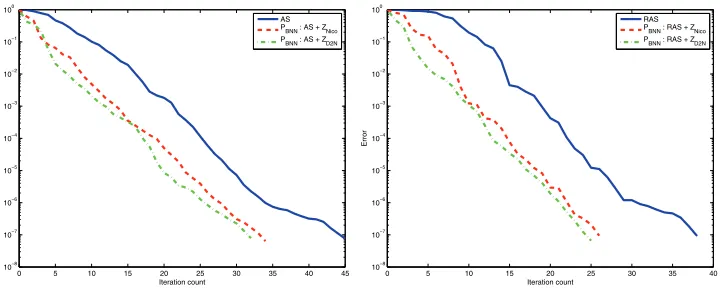
4.2.1. Homogeneous viscosity. In this case we have _κ= 1 in the whole do-main. As in the case of a one-way decomposition, the two preconditioning methods based on Nicolaides coarse grid and DtN eigenvectors behave in quite a similar way whether AS or RAS are used when the viscosity is constant in the whole domain. Here we have chosen a 4×4 regular subdomain decomposition. Each subdomain has 40 nodes on each side, and the overlap equals 2 elements. As expected, using the new algorithm, the number of eigenvectors contributed by each subdomain (which is

0 5 10 15 20 25 30 35 40 45 10−8 10−7 10−6 10−5 10−4 10−3 10−2 10−1 100 Iteration count Error AS P

BNN : AS + ZNico

P

BNN : AS + ZD2N

0 5 10 15 20 25 30 35 40

10−8 10−7 10−6 10−5 10−4 10−3 10−2 10−1 100 Iteration count Error RAS P

BNN : RAS + ZNico

P

BNN : RAS + ZD2N

Fig. 4.9_{. 4}×_{4subdomains, uniformκdistribution, for AS (left) and RAS (right).}

IsoValue -52630.5 26316.8 78948.3 131580 184211 236843 289474 342106 394737 447369 500001 552632 605264 657895 710527 763158 815790 868421 921053 1.05263e+06 IsoValue -47367.4 23685.2 71053.6 118422 165790 213159 260527 307895 355264 402632 450001 497369 544737 592106 639474 686842 734211 781579 828947 947368

Fig. 4.10_{.Heterogeneous viscosity: alternating (left) and skyscraper (right) cases.}

calculated automatically) is always 1. Figure 4.9 shows all three convergence curves for both AS and RAS. This numerically asserts that in the constant coefficient case

the_{ZN ico} and _ZD2N are almost identical. The small differences lie in the fact that

for_{ZN ico}the coarse space is defined analytically, whereas for_ZD2N it is obtained via

a numerical procedure.

4.2.2. Highly heterogeneous viscosity. We will perform the same tests as before on two different configurations of highly heterogeneous viscosity. We consider the following situations:

• alternating viscosity: for_ysuch that for [9_y]≡0(mod 2),_κ= 106; and_κ= 1 elsewhere. (See Figure 4.10(left).)

• skyscraper viscosity: for _x and_y such that for [9_x] ≡0(mod 2) and [9_y] ≡ 0(mod 2),_κ= 105·([9_y] + 1); and_κ= 1 elsewhere. (See Figure 4.10(right).) Here the number of eigenvectors considered in the construction of the coarse space is more important than in the homogeneous case (otherwise the global information cannot be correctly captured), and it may vary as a function of the number of subdo-mains. In the alternating case we used two or three modes per subdomain, whereas for the skyscraper case we used between two and four eigenvectors per subdomain. Note that for each subdomain the total number of eigenvalues is equal to the number of nodes on the interface. In these cases, typical values are 2, 3, or 4. Table 4.4 shows that using the new method highly improves convergence whether a uniform or

Table 4.4

Convergence results for the skyscraper and alternating test cases.

AS AS+Nico AS+D2N RAS RAS+Nico RAS+D2N

Alternating 65 76 29 51 57 16

Metis alt. 101 90 37 83 67 23

Skyscraper 344 360 18 185 183 10

Metis sky. 375 968 28 164 158 19

Fig. 4.11_{. 4}×_{4subdomains uniform (left) and Metis (right). This shows both the subdomain}

boundaries and the jumps inκfor the “hard” test case.

0 20 40 60 80 100 120 140 160 180 10−9

10−8

10−7

10−6 10−5

10−4

10−3

10−2

10−1

100

101

Iteration count

Error

RAS P

BNN : RAS + ZNico

P

BNN : RAS + ZD2N

0 50 100 150

10−8

10−7

10−6

10−5

10−4

10−3 10−2

10−1

100

101

Iteration count

Error

RAS P

BNN : RAS + ZNico

P

BNN : RAS + ZD2N

Fig. 4.12. 4×4subdomains, uniform (left) and Metis (right)—RAS convergence for the “hard”

test case.

Metis partition is used in this highly heterogeneous coefficient case. The Nicolaides preconditioner gives results comparable to those of the one-level method.

4.2.3. A hard test case with inclusions and channels. In order to compare our method to existing codes we solve a test case with known difficulties: the diffusion coefficient_κtakes values between 1 and approximately 1_.5×106, and the distribution contains both inclusions and channels. The total number of nodes will always be 256 on each side of Ω. The decomposition will change, however: we will successively consider a 2×2 decomposition, a 4×4 decomposition, and an 8×8 decomposition.

noverlapswill always be equal to 2. As an illustration, we have chosen to present the 4×4 case extensively both with and without using the Metis partitioner.

Figure 4.11 shows together the decomposition into subdomains and the jumps in

κ; Figure 4.12 shows the convergence curves for the three methods using RAS. We

Table 4.5

Convergence results for the hard test case.

AS AS+Nico AS+D2N RAS RAS+Nico RAS+D2N

2×2 103 110 22 70 70 14

2×2 with Metis 76 76 22 57 57 18

4×4 603 722 26 169 165 15

4×4 with Metis 483 425 36 148 142 23

8×8 461 141 34 205 95 21

8×8 with Metis 600 542 31 240 196 19

IsoValue -31754.4

20877.2 55964.9 91052.6

126140

161228

196316 231404

266491 301579

336667 371754 406842 441930 477018

512105

547193

582281 617368

705088

0 10 20 30 40 50 60

10−8

10−7

10−6

10−5

10−4 10−3

10−2

10−1

100

Iteration count

Error

RAS PBNN : RAS + ZNico

P

BNN : RAS + ZD2N

Fig. 4.13. Metis4×4 subdomains—κ for the “continuous” test case (left) and convergence

history (right).

Table 4.6

Condition numbers for the continuous test case,8×8decomposition with Metis.

Condition number Smallest eigenvalue Largest eigenvalue

AS 4.566043e+03 8.760321e-04 4.000000e+00

AS + Nicolaides 1.127232e+02 3.547273e-02 3.998598e+00

AS + D2N 1.469540e+01 2.717523e-01 3.993508e+00

used between one and four eigenvectors per subdomain because the heterogeneities in _κimpose that more global information on the solution be exchanged to avoid the plateau phenomenon. The convergence curves show that this strategy is a success; results are summarized in Table 4.5.

4.2.4. Continuous variations of the coefficient. This time we take an ana-lytical function for_κwhich is chosen as

κ(_{x, y}) =_κM/3 sin(_{ω π}(_x+_y) + 0_.1)_.

In our case_κM= 106and_ω= 4. We chose a two node overlap and a total of 160 nodes per side of the global domain. We study the 4×4 and 8×8 decompositions both with and without Metis. As an example, Figure 4.13 shows information for the 4×4 decomposition using Metis. Table 4.6 shows information on the approximate condition numbers of the preconditioned operators in the Metis 8×8 case. This was achieved using the Ritz values during the CG iteration procedure when AS is used. As expected for D2N, the smallest eigenvalue is larger than in the other cases, which leads to a better condition number for the operator. Finally, Table 4.7 shows the number of iterations needed to reach convergence for all three methods in all four

Table 4.7

Convergence for the continuous test case.

AS AS+Nico AS+D2N RAS RAS+Nico RAS+D2N

4×4 57 46 32 48 35 23

4×4 with Metis 64 48 30 53 41 24

8×8 461 141 34 205 95 21

8×8 with Metis 600 542 31 240 196 19

IsoValue -4.86701

-3.74453 -2.9962 -2.24787

-1.49955

-0.751221

-0.00289558 0.74543

1.49376 2.24208

2.99041 3.73873 4.48706 5.23539 5.98371

6.73204

7.48036

8.22869 8.97702

10.8478

0 10 20 30 40 50 60

10−8

10−7

10−6

10−5

10−4 10−3

10−2

10−1

100

Iteration count

Error

AS PBNN : AS + ZNico

P

BNN : AS + ZD2N

Fig. 4.14.log(κ)for the random test case (left) and convergence history (right) for AS with an

overlap of2.

Table 4.8

Condition numbers for the random test case and overlap= 2.

Condition number Smallest eigenvalue Largest eigenvalue

AS 5.765809e+02 6.937447e-03 4.000000e+00

AS + Nicolaides 1.665329e+02 2.401928e-02 4.000000e+00

AS + D2N 1.635163e+01 2.445822e-01 3.999317e+00

cases. Again D2N performs significantly better.

In this section we propose a test with random coefficient. We use a log-normal distribution for the parameter _κ. This distribution is calculated using the Gaussian random field generator available at [12]. We choose the exponential covariance family with parameters _θ2 = 1 and _θ1 = _e−1λ with _λ = 4Δ_x in order for the correlation

r(_l) between the values at two points separated by a distance _l to be _r(_l) = _e−λl. This gives us a normal distribution with mean value 0 of the random variable_X at each grid point. We then define_X =_σX +_μin order to have a _μmean value and a _σ standard deviation. In our example, _μ = 3 and _σ = 2 (see Figure 4.14(left)). Finally, we calculate_κ= 10X, giving us a log-normal random field with mean value

μκ=μln(10) and standard deviationσκ=σln(10).

4.2.5. Random κ distribution. The parameters of the test case are the fol-lowing: 4×4 subdomains, 20 nodes per subdomain edge, using a Metis partition. For these values_λ= 4∗ _4×1₂₀ = 0_.05. The size of the overlap will be successively 1, 2, and 3, and we will compare the RAS and AS methods. The size of the overlap does not have a significant influence on the comparison between methods, as shown in Table 4.9. In order to improve the condition number (Table 4.8) as many as 9 out of 99 eigenvectors are used to build the coarse space, with success.

Table 4.9

Convergence for the random test case (4×4decomposition with Metis).

AS AS+Nico AS+D2N RAS RAS+Nico RAS+D2N

Overlap = 1 89 82 30 79 78 22

Overlap = 2 59 57 27 50 52 33

Overlap = 3 45 46 22 36 40 24

5. Conclusions. We have considered the extended (2.2) and the original (2.1) linear systems arising from the domain decomposition method with overlap. We applied the two-level preconditioner using the Schwarz algorithm and the coarse-grid correction. The coarse-grid space is based on the low-frequency modes of the local DtN map. Its size automatically adapts to the difficulty of the problem. With this coarse space, we can obtain fast convergence for problems with large discontinuities (even along the interface) and arbitrary domain decompositions. The method has the potential to be extended to other systems of equations like elasticity, but it requires further investigation.

REFERENCES

[1] J. H. Bramble, J. E. Pasciak, and A. H. Schatz_{,The construction of preconditioners for}

elliptic problems by substructuring, I, Math. Comput., 47 (1986), pp. 103–134.

[2] X.-C. Cai and M. Sarkis,A restricted additive Schwarz preconditioner for general sparse

linear systems, SIAM J. Sci. Comput., 21 (1999), pp. 792–797.

[3] A. St-Cyr, M. J. Gander, and S. J. Thomas_{,Optimized multiplicative, additive, and}

re-stricted additive Schwarz preconditioning, SIAM J. Sci. Comput., 29 (2007), pp. 2402– 2425.

[4] C. R. Dohrmann and O. B. Widlund,An overlapping Schwarz algorithm for almost

incom-pressible elasticity, SIAM J. Numer. Anal., 47 (2009), pp. 2897–2923.

[5] C. R. Dohrmann and O. B. Widlund_{,Hybrid domain decomposition algorithms for}

compress-ible and almost incompresscompress-ible elasticity, Internat. J. Numer. Methods Engrg., 82 (2010), pp. 157–183.

[6] M. Dryja, M. V. Sarkis, and O. B. Widlund_{,Multilevel Schwarz methods for elliptic}

prob-lems with discontinuous coefficients in three dimensions, Numer. Math., 72 (1996), pp. 313– 348.

[7] E. Efstathiou and M. Gander_{,Why restricted additive Schwarz converges faster than}

addi-tive Schwarz, BIT, 43 (2003), pp 945–959.

[8] Y. A. Erlangga and R. Nabben,Deflation and balancing preconditioners for Krylov

sub-space methods applied to nonsymmetric matrices, SIAM J. Matrix Anal. Appl., 30 (2008), pp. 684–699.

[9] Y. A. Erlangga and R. Nabben_{,Algebraic multilevel Krylov methods, SIAM J. Sci. Comput.,} 31 (2009), pp. 3417–3437.

[10] J. F. Escobar_{,The geometry of the first non-zero Stekloff eigenvalue, J. Funct. Anal., 150} (1997), pp. 544–556.

[11] G. Karypis and V. Kumar_{,METIS—Unstructured Graph Partitioning and Sparse Matrix}

Ordering System; see http://glaros.dtc.umn.edu/gkhome/views/metis.

[12] B. Kozintsev and B. Kedem_{,Clipped Gaussian random fields, field generating software, 1999,}

available online at http://www-users.math.umd.edu/∼bnk/bak/generate.cgi.

[13] F. Magoul`es, F.-X. Roux, and L. Series,Algebraic approximation of Dirichlet-to-Neumann

maps for the equations of linear elasticity, Comput. Methods Appl. Mech. Engrg., 195 (2006), pp. 3742–3759.

[14] J. Mandel_{, Balancing domain decomposition, Comm. Numer. Methods Engrg., 9 (1993),} pp. 233–241.

[15] J. Mandel and M. Brezina_{,Balancing domain decomposition for problems with large jumps}

in coefficients, Math. Comp., 65 (1996), pp. 1387–1401.

[16] F. Nataf, F. Rogier, and E. de Sturler_{,Optimal Interface Conditions for Domain}

Decom-position Methods, Internal Report 301, CMAP (Ecole Polytechnique), Palaiseau, France,

1994; available online at http://www.ann.jussieu.fr/∼nataf/cvfiniMod.pdf.

[17] R. A. Nicolaides_{,Deflation of conjugate gradients with applications to boundary value}

prob-lems, SIAM J. Numer. Anal., 24 (1987), pp. 355–365.

[18] A. Padiy, O. Axelsson, and B. Polman_{,Generalized augmented matrix preconditioning}

ap-proach and its application to iterative solution of ill-conditioned algebraic systems, SIAM J. Matrix Anal. Appl., 22 (2000), pp. 793–818.

[19] C. Pechstein and R. Scheichl_{,Scaling up through domain decomposition, Appl. Anal., 88} (2009), pp. 1589–1608.

[20] C. Pechstein and R. Scheichl_{, Analysis of FETI methods for multiscale PDEs, Numer.} Math., 111 (2008), pp. 293–333.

[21] O. Pironneau, F. Hecht, A. Le Hyaric, and J. Morice_{,FreeFem++, Laboratoire J.-L.} Li-ons; available online at http://www.freefem.org/ff++/.

[22] Y. Saad and M. H. Schultz,GMRES: A generalized minimal residual algorithm for solving

nonsymmetric linear systems, SIAM J. Sci. Stat. Comput., 7 (1986), pp. 856–869. [23] B. E. Smith and P. E. Bjøstad_{, Domain Decomposition: Parallel Multilevel Methods for}

Elliptic Partial Differential Equations, Cambridge University Press, Cambridge, UK, 1996. [24] J. M. Tang, R. Nabben, C. Vuik, and Y. A. Erlangga_{,Comparison of two-level}

precon-ditioners derived from deflation, domain decomposition and multigrid methods, J. Sci. Comput., 39 (2009), pp. 340–370.

[25] J. M. Tang, S. P. MacLachlan, R. Nabben, and C. Vuik_{,A comparison of two-level}

pre-conditioners based on multigrid and deflation, SIAM. J. Matrix Anal. Appl., 31 (2010), pp. 1715–1739.

[26] A. Toselli and O. Widlund_{, Domain Decomposition Methods: Algorithms and Theory,}

Springer, New York, 2005.

[27] C. Vuik, A. Segal, and J. A. Meijerink_{, An efficient preconditioned CG method for the}

solution of a class of layered problems with extreme contrasts in the coefficients, J. Comput. Phys., 152 (1999), pp. 385–403.

[28] C. Vuik, A. Segal, J. A. Meijerink, and G. T. Wijma,The construction of projection vectors

for a deflated ICCG method applied to problems with extreme contrasts in the coefficients, J. Comput. Phys., 172 (2001), pp. 426–450.