Detection of cracks in simply-supported beams by continuous wavelet transform of reconstructed modal data

Detection of cracks in simply-supported beams by

continuous wavelet transform of reconstructed modal data

Shuncong Zhong 1,2 _{and S Olutunde Oyadiji} 3*

1. School of Mechanical Engineering and Automation, Fuzhou University, 350108. P. R. China

2. Department of Electrical Engineering and Electronics, The University of Liverpool, Liverpool L69 3GJ, UK

3. Dynamics and Aeroelasticity Group, School of Mechanical, Aerospace and Civil Engineering, The University of Manchester, M13 9PL, UK

Abstract

This paper proposes a new approach for damage detection in beam-like structures with

small cracks, whose crack ratio (r Hc/H) is less than 5%, without baseline modal

parameters. The approach is based on the difference of the Continuous Wavelet

Transforms (CWTs) of two sets of mode shape data which correspond to the left half

and the right half of the modal data of a cracked simply supported beam. The mode

shape data of a cracked beam, are apparently smooth curves, but actually exhibit local

peaks or discontinuities in the region of damage because they include additional

response due to the cracks. The modal responses of the damaged simply-supported

beams used are computed using the finite element method. The results demonstrate the

efficiency of the proposed method for crack detection, and they provide a better crack

crack location and sampling interval are examined. The simulated and experimental

results show that the proposed method has great potential in crack detection of

beam-like structures as it does not require the modal parameter of an uncracked beam as

a baseline for crack detection. It can be recommended for real applications.

Keywords

Beams, Crack Detection, Damage detection, Continuous Wavelet Transform, Modal

data

1. Introduction

The interest in the ability to monitor a structure and detect damage at the earliest

possible stage is pervasive throughout the civil, mechanical and aerospace engineering

communities. During the past two decades, a variety of analytical, numerical and

experimental investigations have been carried out on cracked structures with a view to

developing robust crack detection methods. Any crack or localized damage in a

structure reduces the stiffness and increases the damping in the structure. Reduction in

stiffness is associated with decreases in the natural frequencies and modification of the

mode shape of the structure. Several researchers have used mode shape measurements

to detect damage. Pandey et al. [1] showed that absolute changes in the curvature mode

shapes are localized in the region of damage and hence can be used to detect damage in

a structure. The change in the curvature mode shapes increase with increasing size of

damage. This information can be used to obtain the amount of damage in the structure.

Ratcliffe [2] found that the mode shapes associated with higher natural frequencies can

be used to verify the location of damage, but they are not as sensitive as the lower

displacements. In fact, the authors of this paper have shown that higher derivatives give

a more sensitive detection [3]. Abdel Wahab and De Roeck [4] investigated the application of the change in modal curvatures to detect damage in a pre-stressed

concrete bridge. They introduced a damage indicator called ’curvature damage factor’.

A crack in a structure introduces a local flexibility that can change the dynamic

behaviour of the structure. Some damage index methods require the baseline data set of

the intact structure for comparison to inspect the change in modal parameters due to

damage. Typically, the baseline is obtained from measurements of the undamaged

structure, As an example, Pandey et al. [1] compared the curvatures of the modes shapes

between the undamaged and damaged structures. Sampaio et al. [5] directly subtracted

the values of the mode shape curvature of the damaged structure from that of the

undamaged structure.

In recent years, the use of wavelet analysis in damage detection has become an area of

research activity in structural and machine health monitoring. The main advantage

gained by using wavelets is the ability to perform local analysis of a signal which is

capable of revealing some hidden aspects of the data that other signal analysis

techniques fail to detect. This property is particularly important for damage detection

applications. A review is provided by Peng and Chu [6] of available wavelet

transformation methods and their application to machine condition monitoring. Deng

and Wang [7] applied directly discrete wavelet transform to structural response signals

to locate a crack along the length of a beam. Tian et al. [8] provided a method of crack

detection in beams by wavelet analysis of transient flexural wave. Wang and Deng [9]

distributed response measurements. The premise of the technique is that damage in a

structure will cause structural response perturbations at damage sites. Such local

perturbations, although they may not be apparent from the measured total response data,

are often discernible from component wavelets. Liew and Wang [10] found that the

presence of cracks can be detected by the change of some wavelet coefficients along the

length of a structural component.

Gentile and Messina [11] were focused on the detection of open cracks in beam

structures that undergo transverse vibrations. They used continuous wavelet transform

to detect the location of open cracks in damaged beams by minimizing measurement

data and baseline information of the structure. Quek et al. [12] examined the sensitivity

of the wavelet technique in the detection of cracks in beam structure. Specially, the

effects of different crack characteristics, boundary conditions, and wavelet functions

used were investigated. Hong et al. [13] presented the effectiveness of the wavelet

transform by means of its capability to estimate the Lipschitz exponent, whose

magnitude can be used as a useful indicator of the damage extent. Damaged beams were

investigated both numerically and experimentally. Yan et al. [14] evaluated the ability

of detecting crack damage in a honeycomb sandwich plate by using natural frequency

and dynamic response. They found energy spectrum of wavelet transform signals of

structural dynamic response has higher sensitivity to crack damage. Douka et al. [15]

used wavelet analysis for crack identification in beam structures. The fundamental

vibration mode of a cracked cantilevered beam was analyzed using wavelet analysis and

both the location and size of the crack are estimated.

energy rate index, for the damage detection of beam structures. The simulated and

experimental studies demonstrated that the wavelet packet transform based energy rate

index is a good candidate index that is sensitive to structural local damage. Chang and

Chen [17] presented a technique for structure damage detection based on spatial wavelet

analysis. Using the technique, the positions and depths of the cracks can be predicted

with acceptable precision even though there are many cracks in the beam. Zumpano and

Meo [18] presented a novel damage detection technique, tailored at the identification of

structural surface damage on rail structures. The damage detection methodology

developed was divided into three steps. The presence of the damage on the structure

was assessed. In the second step, the arrival time of the reflected wave (or echo) was

estimated using Continuous Wavelet Transform (CWT). Then, the detection algorithm

was able, through a ray-tracing algorithm, to estimate the location of damage. Kim et al.

[19] proposed a vibration-based damage evaluation method that can detect, locate, and

size damage using multi-resolution wavelet analysis. Zhu and Law [20] presented a new

method for crack identification of bridge beam structures under a moving load based on

wavelet analysis. The proposed method is validated by both simulation and experiment.

Locations of multiple damages can be located accurately, and the results are not

sensitive to measurement noise, speed and magnitude of moving load, measuring

location, etc.

This paper is aimed at detecting and locating cracks in damaged beams with small

cracks, whose crack ratio is less than 5%. As stated in the previous paragraph, the

minimum value of crack ratios using existing methods of crack detection is 5%. Even

then, the existing methods only provide clear crack detection at crack ratio of 20% or

clear crack identification at crack ratios as small as 5% and even smaller. This new

approach is based on finding the difference of the CWTs of the two sets of mode shape

data. Those two modal data sets, which constitute two new signal series, are obtained

and reconstructed from the modal displacement data of a cracked simply-supported

beam. They represent the left half and the modified right half of the modal data of the

simply supported beam. The left half of the modal data is the left half segment of the

original mode shape data. For a symmetric mode shape, the modified right half modal

data is obtained from rotating the right half segment of the mode shape about the

vertical axis which passes through the centre of the mode shape, that is the vertical

centre of the beam. For an antisymmetric mode shape, the modified right half segment

is produced by rotating the right half of the mode shape twice: firstly about the vertical

axis and secondly about the horizontal axis which pass through the centre of the mode

shape.

CWT algorithm is firstly introduced in this paper. Then, a numerical example is

provided to illustrate the operation of the method. This partly involves the computations

of the first few natural frequencies and mode shapes of cracked simply supported beams

using the ABAQUS finite element code. For brevity, only CWT of the first four mode

shapes is investigated. The original mode shape data or ‘signal’ is divided and

reconstructed into two signal series; one is the first half of the original mode shape

‘signal’, the other is a modified signal obtained from the second half of the original

mode shape ‘signal’. To further verify the efficiency and practicability of the proposed

method, the effects of crack location, mode shape data sampling interval are

investigated. The simulated and experimental results show that the proposed method has

recommended for real applications.

2. Continuous wavelet transform

This section presents a brief background on continuous wavelet transform utilized in

this paper. More facts on continuous wavelet transform can be found in the study of

Daubechies [21].

A mother wavelet (x) can be defined as a function with zero average value,



) (x

 is normalized:

1 )

( 2 



From mother wavelet (x), the analyzing wavelets can be obtained by dilation

parameter s and translation parameter b:

) ( 1 ) ( , s b x s x s b   

 (3)

where both s and b are real numbers, and s must be positive.

The continuous wavelet transform of a signalf(x)L2(R)depending on time or space,

is defined by



Wf)( , ) ( ) 1 ( )

where (*) denotes the complex conjugate, the mother wavelet should satisfy an

admissibility condition to ensure existence of the inverse wavelet transform, such as

  

_

where F_() denotes the Fourier transform of (x)defined as



 _

 x e dx x R

F_() ( ) ix , (6)

The signal f(x) may be recovered or reconstructed by an inverse wavelet transform

of )Wf(s,b defined as

 

 



 1 ( )( , ) ( ) ₂

) ( s dsdb s b x b s Wf C x f   (7)

Also, the CWT may as well be performed in Fourier space [22]



   

 F e F s d

b s

Wf f ( ) ib ( )

2 1 ) , )(

( * (8)

where F_f() is the Fourier transform of f(x)defined as



 _

 f x e dx x R

F_f() ( ) ix , (9)

The local resolution of the CWT in time or space and in frequency depends on the

dilation parameter s and is determined, respectively, by the duration x_ and

s x

s

x  _   

 , (10)

Here, x_ and _ are defined as

dx x x

x x

x



   

 ₂ 2

2 ) ( ) ( ) ( 1 _  

 (11)

      _{ } 

 F d

F



   



 ₂ 2

2 ) ( ) ( ) ( 1 (12)

where x_ and _ are the centre of (x) and F_(), respectively,

dx x x x x



   ₂ 2 2 ) ( ) (  

 (13)

        d F F



 denotes the classical norm in the space of square integrable functions.

It is well known that the number of vanishing moments is one of the most important

factors for the success of wavelets in various applications [24]. In the present work, a

symlet wavelet ‘symmetrical 4’ having four vanishing moments has been selected and

used as the analyzing wavelet. The scaling function and wavelet function of

‘symmetrical 4’ wavelet are shown in Fig.1 (a) and (b).

detectable when the cracks are in the early state. This method uses the difference of the

CWTs of two reconstructed sets of data or signal series obtained from the original mode

shape of a cracked beam. Firstly, the original mode shape signal is divided and

reconstructed into two signal series as follows. If the original mode shape ‘signal’ is

made up ofd1,d2,...,dN data points, where N is the total number of sampling points,

the first segment (s₁') of the signal is the first half of the original mode shape ‘signal’,

that is, d1,d2,...dN/21. The second segment ( ' 2

s ) of the signal is the second half of the

original mode shape ‘signal’, that is, d_N/21,d_N/22,...,d_N. This process of dividing and

reconstituting the signals is illustrated in Fig.2 (a-1) and (a-2) for modes 1 and 2,

respectively, of the beam. There are two cases, namely symmetric and antisymmetric

cases. For symmetric cases, the mode shape is symmetrical about the centre of the beam,

as illustrated in Fig.2 (a-1) for the first mode. In this case, the modal data is cut into left

and right segments s₁' and s₂', respectively. The right modal data segment is rotated

about a vertical axis to produce a modified data set s₂ which is similar to the left

modal data segment s1. The two new signal series s1 and s2 are obtained as

1 2 / 2

1,d ,...,dN 

d (the signal seriess1) and dN,dN1,...,dN/21(the signal seriess2), as

shown in Fig.2 (b-1). For antisymmetric cases, the mode shape is antisymmetrical about

the centre of the beam as illustrated in Fig.2 (a-2) for the second mode. In this case, the

right data segment is rotated twice: firstly about the vertical axis and secondly about the

horizontal axis to produce a modified data set s2. Thus, the two signal series will be

1 2 / 2

1,d ,...,dN 

d (the signal seriess₁) and dN,dN_1,...,dN_/21 (the signal seriess2),

Then the wavelet coefficients, the difference of CWT of s₁ and s₂, will be obtained

after CWTs of s₁ and s₂ are performed. For the case of a beam with small cracks,

CWT of s1 or s2 includes some crack information. However, due to the smallness of

the crack, the distortion of the transformed data caused by the crack is not very

significant and, therefore, can not provide a clear crack detection. Finally, the difference

of the CWT of s1 and s2 is determined to give a better crack indication than the

CWT of the original mode shape. However, it is noted that the proposed method is only

suitable for the simply supported beams with symmetric and antisymmetric mode

shapes.

4. Numerical example

4.1 Finite element modal analysis

In order to illustrate the applicability of the proposed method for crack detection, the

natural frequencies and mode shapes of simply-supported cracked beams are computed

using the ABAQUS finite element code. A simply supported beam with a single-sided

transverse crack with a fixed depthH_c, a crack widthW_c, and located at distance

c

l from the left support is shown in Fig.3. A mild steel beam of breadth b=100 mm,

depth H=25 mm and length L=3000 mm was modeled using 20 node 3D brick

element which is denoted in the ABAQUS FE package as C3D20R. The material

properties of the beam are: Young’s modulusE210GPa, Density 7850Kg/m3,

Poisson’s ratiov0.3. In the FE model, the axial length of elements used in the

analysis was le= 5mm for a 3000 mm long cracked beam when the elements are not

location as shown in Fig.4. The first 50 natural frequencies and mode shapes of

damaged and intact beams are computed.

The cracks are 0.1 mm wide and 1 mm deep and are located at 500 mm, 1000 mm, 1500

mm, 2000 mm and 2500 mm from the left end of the beam. The crack ratio of all the

beams is 4%. Three sampling distances of the mode shape data are studied, namely,

s

x

= 5, 25 and 50 mm. For the case of sampling distance 5 mm, the modal displacement

data is sampled (from the top beam surface) at 5 mm interval along the lengths of the

beams resulting in a total of 601 data points. But this represents too much measurement.

Therefore, the cases of sampling distances of 25 mm and 50 mm, which are closer to

real applications, are also studied.

4.2 Comparison of CWT of original mode shape data with difference of CWTs

The method proposed in the present work is compared with the method using CWT

of the original mode shapes in the following part of this section. Fig.5 (a) to (d) show

the wavelet coefficients of the original first, second, third and fourth mode shapes of the

damaged beam with the crack located at 500 mm from the left end of the beam, and for

a sampling distance of 5 mm. Four scales were used for analysis, namely: s5, 15, 25

and 35.

For modes 1 to 3, Fig. 5(a) to (c) provide obvious (unambiguous) evidence of crack

existence at 500 mm from the left end of the cracked beam only when the wavelet scale

is equal to or greater than 25 (i.e. s  25). But when s < 25, the figures do not provide

very obvious evidence of crack existence. In fact, for mode 4, Fig.5 (d) shows very little

Fig.6 (a) to (d) show the difference of the wavelet coefficients of s₁ and s₂ obtained

from the first, second, third and fourth mode shape ‘signals’, respectively, of the

damaged beam. All the figures provide evidence of crack existence at 500 mm from the

left end of the beam because all the wavelet coefficients exhibit high peak values at this

position. The results of the proposed method give better crack indication than those of

the method using the CWT of the original mode shape data shown in Fig.5.

To be certain about the presence of the crack, however, one has to examine in detail the

behaviours of the wavelet maxima at these points as the scale increases. Fig. 7 presents

3D and contour plots of the CWT coefficients of the original mode shape data for scales

1–48 of the first four mode shape data. It is seen that none of the figures clearly

identifies the crack and its location.

Fig.8 (a-1) to (d-1) are the 3D plots of the difference of the CWT coefficients of the two

signal series s₁ and s₂ for the first four mode shape data of the damaged beam.

Similarly, Fig.8 (a-2) to (d-2) are the contour plots of the difference of the CWT

coefficients of the two signal series s1 and s2. The figures show very clear evidences

of crack existence at 500 mm.

It can be seen from Fig.8 that the absolute value of the modified wavelet maxima

increases in a regular manner with increasing scale. Also, the absolute value of the

wavelet maxima of higher mode shape data is greater than that of lower mode shape

data. Comparing all the figures in Fig.7 and Fig.8, an important conclusion can be

obtained that the difference of the CWT coefficients of s₁ and s₂ gives better crack

wavelet maxima of higher original mode shape is also greater than that of lower original

mode shape. In fact, the increase in magnitude of the coefficients for original mode

shape and difference of mode shape is due to the fact that damage induced local

response is easy to be captured by the higher modes [25]. Typically, damage is a local

phenomenon. Local response is captured by higher frequency modes whereas lower

frequency modes tend to capture the global response of the structure and are less

sensitive to local changes in a structure [26].

5. Further verification of the proposed method in crack detection

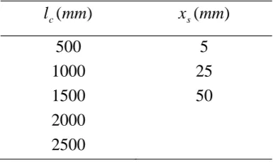
To verify the efficiency and practicability of the proposed method, a further 15 cases

with cracks of varying location and using different sampling distances, as shown in

Table 1, are studied. In this section, the effects of crack location and spatial intervals

(sampling distances) of mode shape data on the difference of continuous wavelet

transform (CWT) coefficients of the new signal series s₁ and s₂ are investigated.

5.1 Effect of crack location

Fig.9 (a-1) to (d-1) are, respectively, the 3D plots of the difference of the CWT

coefficients of the two signal series s₁ and s₂ obtained from the first, second, third

and fourth mode shape data of the damaged beam with the crack located at l_c = 1000

mm.

Fig.9 (a-2) to (d-2) show the corresponding contour plots of the difference of the CWT

coefficients of the two signal series s1 and s2 obtained from the first four mode

shape data of the damaged beam. There are obvious evidences of crack existence at

wavelet difference maxima increases in a regular manner with increasing scale. Also,

the absolute value of the wavelet difference maxima of higher mode shape data is

greater than that of lower mode shape data. The absolute value of the wavelet difference

maxima of the first mode shape for the case of a crack located at 1000 mm is greater

than that of the case of a crack located at 500 mm. However, the absolute value of the

wavelet difference maxima of the second mode shape for the case of a crack located at

1000 mm is equal to that of the case of a crack located at 500 mm. The reason is that the

modal displacements of points far away from the node of a mode are greater than those

of points close to the node of the mode. Thus, in the case of mode 1, the CWT at 1000

mm is greater than that at 500 mm because location lc = 1000 mm is further away

from a node than location l_c = 500 mm. But in the case of mode 2, the CWT at 1000

mm is equal to that at 500 mm because locations l_c = 1000 mm and l_c = 500 mm are

equidistant from the nodes of the mode shape of mode 2. For mode 3, the crack location

is the node of the mode, therefore, the modal displacement for this case is close to zero,

as shown in Fig.9 (c-1) and (c-2).

All the above discussion is focused on cracks located at the left part of the beam. A

crack located at the right part of the beam is also investigated. Fig.10 (a-1) to (d-1) are,

respectively, the 3D plots of the difference of the CWT coefficients of the two signal

series s₁ and s₂ obtained from the first four mode shape data of the damaged beam

with a crack located at 2000 mm from the left end of the beam. Fig.10 (a-2) to (d-2)

show the corresponding contour plots of the difference of the CWT coefficients of the

two signal series s₁ and s₂ for the first four mode shapes of the damaged beam.

all the other figures indicate discontinuities at location 1000 mm which suggest the

presence of a crack at this location. However, this is a pseudo location. The real location

is at 2000 mm which is the mirror image of location 1000 mm. Also, in this case, the

wavelet difference maxima are negative. However, the conclusion is still that the

absolute value of the wavelet difference maxima increases in a regular manner with

increasing scale. Furthermore, the absolute value of the wavelet maxima of higher mode

shape data is greater than that of lower mode shape data.

When the crack is located at 2500 mm from the left end of the damaged beam, the 3D

plots of the difference of the CWT coefficients of the two signal series s₁ and s₂

obtained from the first four mode shape data are shown in Fig.11 (a-1) to (d-1),

respectively, while Fig.11 (a-2) to (d-2) show the corresponding contour plots of the

difference of the CWT coefficients. These figures clearly indicate the presence of a

crack at location 500 mm which is the mirror image of the actual location. Comparing

Fig 11 (a-1) to (d-1) with Fig 8(a-1) to (d-1), respectively, it is seen that when the crack

is located at lc = 500 mm, the maxima of the difference of the CWT coefficient is

positive. But when the crack is located at l_c = 2500 mm, the maxima of the

difference of the CWT coefficient is negative. Therefore, the sign of the maxima of

the difference of the CWT coefficient can be used to identify whether a crack is located

on the left or right half of the simply-supported beam.

From the above discussion, it may be construed that the proposed method can only give

good crack indication when the crack is not located at the centre of a beam. A legitimate

question may be posed as to whether the proposed method is suitable for the special

A beam with a crack located at 1500 mm (the beam centre) from the left end of the

beam, whose width and depth are 0.1 mm and 1 mm, respectively, is considered. The

other parameters are the same as for the beams discussed previously. The original mode

shapes are sampled at 5 mm interval along the lengths of the beams. Fig.12 (a-1) to (d-1)

show the 3D plots of the difference of the CWT coefficients of the two signal series s1

and s₂ obtained from the first four mode shape data. The corresponding contour plots

of the difference of the CWT coefficients are shown in Fig.12 (a-2) to (d-2). It can be

seen from Fig.12 (a-1), (a-2), (c-1) and (c-2) that there is no crack information

manifested in the difference of the CWT transform coefficient of the two signal series

1

s and s₂ obtained from the first and third mode shapes. However, Fig.12 (b-1), (b-2),

(d-1) and (d-2) show that the difference of the CWT coefficients for the second and

fourth mode shapes indicates the presence of crack near the middle of the beam.

The principle of the proposed method results in the above observation which is

summarized in the following. The first mode shape of a cracked simply-supported beam

is a symmetrical one, and the two new signal seriess₁ (d₁,d₂,...,d_N/21) and s₂

(dN,dN1,...,dN/21) are almost the same. Consequently, the difference between the

CWT coefficient of s1 and s2 obtained from the first mode shape is very small. As

for the second mode shape of a cracked simply-supported beam, it is an antisymmetrical

one; the two new signal series s₁ (d₁,d₂,...,d_N/21) and s₂ (d_N,d_N1,...,d_N/21)

have some difference in the cracked area. Hence, the difference of the CWT coefficients

of s₁ and s₂obtained from the second mode shape can give some crack information.

The results can be seen from Fig.12 (b-1), and (b-2), which give obvious peak in the

the CWT coefficients of the second mode shape is very small being of the order of108.

However, all the previous figures show that for a crack located away from the centre,

the magnitude of the CWT coefficient difference is much greater than108. The reason

for the very small magnitude of the CWT coefficient difference when the crack is

located at the centre of the beam is due to the fact that the modal displacements of the

second mode shape near the centre are very small in magnitude because the centre of

the beam is a node for mode 2 of vibration. This results in the difference of the CWT

coefficients of s1 and s2obtained from the second mode shape being also small in

magnitude. Nevertheless, the difference of the CWT coefficient of the second mode

shape can still give crack information for damage detection.

Similarly, it was observed that the CWT coefficient difference of the third mode shape

data gave no crack information whereas the CWT coefficient difference of the fourth

mode shape data gave crack information. Thus, it can be generalized that when a crack

is located at the centre of a simply-supported beam, the difference of the CWT

coefficient of the symmetrical mode shapes will not provide crack information; only the

difference of the CWT coefficient of the antisymmetrical mode shapes will provide

crack information.

5.2 Effect of sampling distance

The results presented in the previous section were based on a sampling interval

(distance) of the mode shape data of 5 mm. When the modal displacement data are

sampled at distance intervals of 25 mm along the length of the beams, it results in a total

In Fig.13 (a-1) to (d-1) are shown the 3D plots of the difference of the CWT coefficients

of the two signal series s1 and s2 obtained from the first four mode shape data of the

same damaged beam. The sampling distance is 25 mm. Fig.13 (a-2) to (d-2) are,

respectively, the corresponding contour plots. The results clearly indicate the presence

of a crack at the correct location of 500 mm.

A larger sampling distance of 50 mm was also investigated. Fig.14 (a-1) to (d-1) are,

respectively, the 3D plots of the difference of the CWT coefficients of the two signal

series s₁ and s₂ obtained from the first four mode shape data of the same damaged

beam. The corresponding contour plots of the difference of the CWT coefficients of the

two signal series s₁ and s₂ are shown in Fig.14 (a-2) to (d-2). The figures show that

the accuracy of the crack location degrades as the sampling distance is increased.

However, the difference of the CWT coefficient still gives reasonable information to

enable crack detection.

5.3 Modified approach for real applications using large sampling distance

As discussed previously, the number of sensors available will be limited. This will result

in large sampling distances. However, the accuracy of the detection of the crack location

degrades as the sampling distance is increased. A larger sampling distance of 75 mm,

which gives a total of 41 measurement points, was investigated.

Fig.15 (a-1) to (d-1) are, respectively, the 3D plots of the difference of the CWT

coefficients of the two signal series s₁ and s₂ obtained from the first four mode

shape data of the same damaged beam. The corresponding contour plots of the

Fig.15 (a-2) to (d-2). Similar to the results using smaller sampling distance (i.e.x_s = 50, 25, and 5 mm), the accuracy of the crack location degrades as the sampling distance is increased.

Now, in order to increase the accuracy of crack detection, before performing a CWT of

the modal data, a spline interpolation is used for the mode shapes which are obtained

using large sampling distances. Subsequently, the difference of the CWT coefficient of

the two signal series s₁ and s₂ which are obtained from the interpolated mode shape

data, is calculated as a damage indicator. The interpolation method can also be found in

the studies of Wang and Deng [9] and Douka et al. [15].

A spline interpolation was applied to each set of 41 measured data points for the first

two mode shapes. The interpolation step was 5 mm, resulting in a total number of 601

derived data points. Fig.16 (a-1) to (d-1) are, respectively, the 3D plots of CWT

coefficients of the first four interpolated mode shape data. Fig.16 (a-2) to (d-2) are,

respectively, the contour plots of the CWT coefficients of the first four interpolated

mode shape data. However, all figures in Fig.16 do not clearly identify the crack nor its

location. Therefore, using only the CWT of the original interpolated mode data can not

provide clear crack indication for small cracks (crack ratio less than 5%) even if the

original modal data is interpolated.

Fig.17 (a-1) to (d-1) are, respectively, the 3D plots of the difference of the CWT

coefficients of the two signal series s₁ and s₂ obtained from the first four

interpolated mode shape data of the damaged beam whose crack depth and width are 1

mm and 0.1 mm. The corresponding contour plots of the difference are shown in Fig.17

Comparing all the figures in Fig.16 and Fig.17, an important conclusion can be obtained

that the modified approach gives better crack indication than the method using the CWT

of the interpolated mode shape data, especially, when the crack ratio is relatively small

(i.e. less than 5%) and the crack effect is small. Also, it can be seen from the figures in

Fig.15 and Fig.17 that the accuracy of the crack detection increases dramatically after a

spline interpolation is used for the mode shapes.

6. Experimental verification of the proposed method in crack detection

Experimental tests using a simply-supported aluminum beam were conducted. The

dimensions of the damaged beam areLHB240025100mm3. A crack, whose

depth is 2.5mm, was located at l_c 0.4m. Fig.18 shows the experimental set-up used

for testing. A random signal was generated and then amplified by a power amplifier, and

exerted on the beam structure through a shaker. The response signal and input signal

were respectively sensed by a PCB (PCB Piezotronics, Inc.) accelerometer and a PCB

force sensor. The displacement data is sampled at 100 mm (x_s 100mm) interval along

the lengths of the beam resulting in a total of 25 data points. Fig.19 shows the first four

normalized measured mode shapes of the cracked beam.

A spline interpolation was applied to each set of 25 measured data points for the first

four mode shapes. The interpolation step was 2 mm, resulting in a total number of 1201

derived data points. Fig.20 (a-1), (b-1), (c-1) and (d-1) show the 3D plots of the

difference of the CWT coefficient of the two signal series s1 and s2 obtained from

the first four interpolated mode shape data of the cracked aluminum beam. The

corresponding contour plots of the difference are shown in Fig. 20 (a-2), (b-2), (c-2) and

From the figures for mode 1 and mode 4, Fig.20 (a-1), (a-2), (d-1) and (d-2), it is seen

that a crack is clearly located at 400 mm from the left end. However, from the figures

for mode 2 and mode 3, due to the experimental noise effect, it is hard to determine the

location of the crack though a peak appears at 400 mm from the left end. To improve the

quality of the results, a simple denoising algorithm was employed: only wavelet

coefficients of value more than 50% of the maximum value are considered. In other

words, a threshold equal to 0.5 of the maximum value has been utilized [15]. The value

of the wavelet coefficient is set to zero if it is less than 50% of maximum value, whilst

the value of the wavelet coefficient is set to the difference between the wavelet

coefficient and 50% of the maximum value if it is greater than 50% of maximum value.

Symbolically, this is expressed as,

        c c c c c c c ˆ 5 . 0 , 0 ˆ 5 . 0 , ˆ 5 . 0 (15)

where c,candcˆ are the original, modified and maximum values of the wavelet

coefficient respectively. It should be noted that this simple algorithm is similar to but

different from the hard-thresholding function used in previous work [27-29].

Fig.21 (a-1 to (d-1) show the 3D plots of the difference of the CWT coefficients whose

values are greater than 50% of the maximum value. The corresponding contour plots of

the difference are shown in Fig. 21 (a-2) to (d-2). It can be seen from Fig.21 (a-1), (a-2),

(d-1) and (d-2) that the improved results show very clear evidences of crack existence at

400 mm because all the wavelet coefficients exhibit high peak values at this position.

However, for the mode 2, Fig.21 (b-1) and (b-2) show two almost equivalent peaks at

located. Furthermore, for the mode 3, Fig.21 (c-1) and (c-2) show the wrong crack

location at 600 mm due to the experimental noise. Here, one conclusion can be obtained

that crack detection cannot only rely on the parameter of one single mode in the real

applications because it is hard to distinguish the crack effect and the noise effect. More

modal parameters should be considered simultaneously.

Secondly, to improve the results further, the number of spatial measurements should be

increased substantially. It was not possible to carry out more measurements in the

present work. Thirdly, in order to reduce the experimental noise effect, the following

equation is proposed to be used as damage index for small crack detection in real

applications,



  N

r r

d d

N A

1 1

(16)

where d_ris the difference of the CWT coefficient of the two signal series s1 and

2

s obtained from the mode shape for mode r, N is the number of mode shapes

considered, Ad is the average of the difference of the CWT coefficient.

Fig.22 (a-1) shows the 3D plot of the average of the difference of the CWT coefficient

of the two signal series s1 and s2 obtained from the first four interpolated mode

shape data of the cracked aluminum beam. The corresponding contour plot of the

average of the difference of the CWT coefficient is shown in Fig. 22 (a-2). The figures

show very clear evidences of crack existence at 400 mm from the left end.

Similarly, the denoising results are shown in Fig.22 (b-1) and (b-2), which are the 3D

contour plot. It follows clearly that the crack is located at l_c 400mm. These

experimental results therefore verify the efficiency and practicability of the proposed

method. It is also noted that the computational time of the proposed method based on

CWT coefficient difference is less than 200 ms and therefore the speed of processing of

experimental data is not an issue. Furthermore, the procedure can be easily made

automatic using Matlab wavelet and signal processing toolboxes, so the proposed

method can be recommended for real monitoring applications.

7. Concluding remarks

This paper proposes a new approach based on the difference of the CWT coefficients of

the two reconstructed signal series to provide a method without baseline modal

parameters for damage detection in beam-like structures with small cracks, whose crack

ratio (r Hc/H) is less than 5%. The two signal series are obtained and reconstructed

from the original mode shape ‘signal’ of a cracked beam. For a beam containing a single

crack, one of these ‘signals’, which is apparently a smooth curve, actually exhibits a

local peak or discontinuity in the region of damage because it includes additional

response due to the crack.

The modal responses of the damaged simply-supported beams used were computed

using the finite element method. Different crack locations and sampling distances were

studied. The results demonstrate the efficiency of the proposed method for crack

detection, and they also provide a better crack indicator than the result of the CWT of

the original mode shape ‘signal’. The simulated results show that the proposed method

Experimental tests using a simply-supported aluminum beam were also conducted in the

present work. In order to improve the accuracy of the crack detection, a spline

interpolation was applied to each set of the measured data points for the first four mode

shapes. The average of the difference of the CWT coefficient of all modes, is used as

damage index for small crack detection in real applications. The experimental results

demonstrate the precision and practicability of the proposed method, which can be

recommended for real applications even when the crack is in the early state.

It should be noted that the use of this method based on CWT requires fairly accurate

estimates of the mode shapes. This is the difficulty for application to real structures.

Generally, to get accurate estimates of the mode shapes, however, one needs detailed

measurements of the mode shapes. This fact increases considerably the duration of the

investigation and this is the main disadvantage of using mode shapes for crack

identification. However, with the availability of fast measurement techniques, such as

scanning laser vibrometer [30], this limitation is not a serious issue. On the other hand,

it has been shown that less detailed measurement can still be used provided that a spline

Appendix A. Nomenclature

c

l crack location of cracked beam from the left support

l length of beams

b width of beams

H depth of beams

c

H crack depth of beams

c

W crack width of beams

E Young’s modulus of material

 _{density of material}

 Poisson ratio of material

e

L element length

r crack ratio

) (x

 mother wavelet function

) ( 

F Fourier transform of (x)

s dilation parameter

b translation parameter

) (x

f analyzed signal

) (

f

) , )(

(W_f s b Continuous wavelet transform of f(x)

 x

 duration of the mother wavelet of (x)





 bandwidth of the mother wavelet of (x)

x

 local resolution of the CWT in time or space



 local resolution of the CWT in frequency



x the centre of (x)



 the centre of F_()

2

 the classical norm in the space of square integrable functions

References

[1] Pandey, A.K., Biswas, M., Samman, M.M., Damage detection from changes in

curvature mode shapes, Journal of Sound and Vibration145 (2) (1991), pp.321-332

[2] Ratcliffe, C. P., Damage detection using a modified Laplacian operator on mode

shape data”, Journal of Sound and Vibration 204 (1997), pp.505-517

[3] Zhong, S., Oyadiji, S. O, “Damage detection in simply supported beams using

derivatives of mode shapes”, Twelfth International Congress on Sound and Vibration,

Lisbon, Portugal (2005), pp.11-14

[4] M.M. Abdel Wahab, Guido De Roeck, Damage detection in bridges using modal

curvatures: application to a real damage scenario, Journal of Sound and Vibration 226(2)

[5] R.P.C. Sampaio, N.M.M. Maia, J.M.M. Silva, Damage detection using the

frequency-response-function curvature method, Journal of Sound and Vibration 226 (5)

(1999), pp. 1029–1042[6] Peng, Z.K., Chu, F.L., Application of the wavelet transform

in machine condition monitoring and fault diagnostics: a review with bibliography,

Mechanical Systems and Signal Processing 18 (2004), pp.199–221.

[7] Deng, X., Wang, Q., Crack detection using spatial measurements and wavelet,

International Journal of Fracture 91 (1998), pp.23-28.

[8] Tian, J.Y., Li, Z., Su, X.Y., “Crack detection in beams by wavelet analysis of

transient flexural waves”, Journal of Sound and Vibration 261 (2003), pp.715-727

[9] Wang, Q., Deng, X., Damage detection with spatial wavelets, International Journal

of Solids and Structures 36 (1999), pp.3443-3468.

[10] Liew, K.M., Wang, Q., Application of wavelet theory for crack identification in

structures, Journal of Engineering Mechanics 124 (1998), 152-157.

[11] Gentile, A., Messina, A., On the continuous wavelet transforms applied to discrete

vibrational data for detecting open cracks in damaged beams, International Journal of

Solids and Structrues 40 (2003), pp.295-315.

[12] Quek, S. T., Wang, Q., Zhang, L., K. Ang, Sensitivity analysis of crack detection in

beams by wavelet technique, International Journal of Mechanical Sciences 43(12)

(2001), pp.2899-2910.

[13] Hong, J. C., Kim, Y. Y., Lee, H. C., Lee, Y. W., Damage detection using the

of a beam, International Journal of Solids and Structures 39 (2002), pp.1803-1816.

[14] Yan, Y.J., Hao, H.N., Yam, L.H., Vibration-based construction and extraction of

structural damage feature index, International Journal of Solids and Structures 41 (2004),

pp.6661-6676.

[15] Douka, E., Loutridis, S., Trochidis, A., “Crack identification in beams using

wavelet analysis”, International Journal of Solids and Structure 40 (2003),

pp.3557-3569

[16] Han, J. G, Ren, W. X., Sun, Z. S., Wavelet packet based damage identification of

beam structures, International Journal of Solids and Structures 42 (2005), pp.6610-6627.

[17] Chang, C. C., Chen, L. W., Detection of the location and size of cracks in the

multiple cracked beam by spatial wavelet based approach, Mechanical Systems and

Signal Processing 19 (2005), pp.139-155.

[18] Zumpano, G. and Meo, M., A new damage detection technique based on wave

propagation for rails, International Journal of Solids and Structures 43 (2006),

pp.1023-1046.

[19] Kim, B. H., Taehyo Park, T., Voyiadjis, G. Z., Damage estimation on beam-like

structures using the multi-resolution analysis, International of Solids and Structures 43

(2006), pp.14-15.

[20] Zhu, X.Q., Law, S.S., Wavelet-based crack identification of bridge beam from

operational deflection time history, International Journal Solids and Structures 43

[21] Daubechies, I., Ten lectures on wavelets, Society for Industrial and Applied

Mathematics, Philadelphia, PA, USA (1992).

[22] Haase, M., Widjajakusuma, J., Damage identification based on ridges and maxima

lines of the wavelet transform, International Journal of Engineering Science 41 (2003),

pp.1423-1443.

[23] Le, T. P., Argoul, P., Continuous wavelet transform for modal identification using

free decay response, Journal of Sound and Vibration 277 (2004), pp.733-100.

[24] Skopina, M., On construction of multivariate wavelets with vanishing moment,

Applied and Computational Harmonic Analysis 20 (2006), pp.375-390.

[25] Qiao, P, Cao, M, Waveform fractal dimension for mode shape-based damage

identification of beam-type structures, International identification of beam-type

structures 45 (2008), pp. 5946-5961.

[26] Farrar, C.R, Doebling, S.W., An overview of modal-based damage identification

methods. In: EUROMECH 365 International Workshop: DAMAS 97, Structural

Damage Assessment Using Advanced Signal Processing Procedures, Sheffield, UK.

[27] Zhong, S., Oyadiji, S. O, “Crack Detection in Simply-Supported Beams without Baseline

Modal Parameters by Stationary Wavelet Transform”, Mechanical Systems and Signal Processing,

21 (2007), pp1853–1884

[28] Zhong, S., Oyadiji, S. O, “Identification of Cracks in Beams with Auxiliary Mass Spatial

Probing by Stationary Wavelet Transform”, ASME Journal of Vibration and Acoustics, 130 (2008),

041001:1-14.

Wavelet Transform of Modal Data”, Structural Control and Health Monitoring (accepted), (2009),

DOI: 10.1002/stc.366

[30] J. Vanherzeele, S. Vanlanduit and P. Guillaume, “Reducing measurement time for

a laser Doppler vibrometer using regressive techniques”, Optics and Lasers in

Fig.1. ‘Symmetrical 4’ wavelet: (a) Scaling function, (b) Wavelet function (mother wavelet)

0 1 2 3 4 5 6 7

-0.25 0.00 0.25 0.50 0.75 1.00 1.25

0 1 2 3 4 5 6 7

-1.2 -0.8 -0.4 0.0 0.4 0.8 1.2 1.6

(a) (b)

Fig.3 Model of cracked simply-supported beam

mm le 0.5

' 

mm le 5

Fig.5 CWT coefficients of the original mode shapes for different scales: W_c 0.1mm,

mm

H_c 1 , x_s 5mm, l_c 500mm, scale = 5, scale =15, scale = 25, scale = 35, (a) mode 1, (b) mode 2, (c) mode 3, and (d) mode 4

(a) (b)

Fig.6 The difference of the CWT coefficients of s1 and s2 for different scales: mm

W_c 0.1 , H_c 1mm , x_s 5mm, l_c 500mm , scale = 5, scale =15, scale = 25, scale = 35, (a) mode 1, (b) mode 2, (c) mode 3, and (d) mode 4

(a) (b)

Fig.7 3D (left) and contour (right) plots of the CWT of the original mode shapes showing the trend of the wavelet modulus maxima for (a) mode 1, (b) mode 2, (c) mode 3, and (d) mode 4; W_c 0.1mm, H_c 1mm, x_s 5mm l_c 500mm

(a-1)

(b-2) (b-1)

(c-1) (c-2)

(d-2) (a-2)

(a-1) (a-2)

(b-2)

(c-2)

(d-2) (b-1)

(c-1)

(d-1)

Fig.8 3D (left) and contour (right) plots of the difference of the CWT coefficients of s1 and

Fig.9 3D (left) and contour (right) plots of the difference of the CWT coefficients of s₁

and s2 showing the trend of the wavelet modulus maxima for (a) mode 1, (b) mode 2, (c)

mode 3 and (d) mode 4; W_c 0.1mm, H_c 1mm, x_s 5mm, l_c 1000mm

(a-1) (a-2)

(b-1) (b-2)

(c-1) (c-2)

(d-1) (d-2)

1.5 1.1 0.7 0.2 -0.1 -0.5 -0.9 -1.3 -1.7 [1E-6]

Fig.10 3D (left) and contour (right) plots of the difference of the CWT coefficients of s1

and s₂ showing the trend of the wavelet modulus maxima for (a) mode 1, (b) mode 2, (c)

   

(a-1) (a-2)

(b-1) (b-2)

(c-1) (c-2)

(d-1) (d-2)

[1E-3] 1.5 0.9 0.4 -0.2 -0.8 -1.3 -1.9 -2.4 -3.0 [1E-6]

Fig.11 3D (left) and contour (right) plots of the difference of the CWT coefficients of s1

and s₂ showing the trend of the wavelet modulus maxima for (a) mode 1, (b) mode 2, (c) mode 3, and (d) mode 4;Wc 0.1mm, Hc 1mm, xs 5mm, lc 2500mm

(a-1) (a-2)

(b-1) (b-2)

(c-1)

(d-1)

(c-2)

(d-2)

[1E-3] 1.5 1.0 0.5 0 -0.5 -1.0 -1.5 -2.0 -2.5 [1E-4]

Fig.12 3D (left) and contour (right) plots of the difference of the CWT coefficients of s₁

and s2 showing the trend of the wavelet modulus maxima for (a) mode 1, (b) mode 2, (c)

(a-1) (a-2)

(b-1) (b-2)

(c-1) (c-2)

(d-1) (d-2)

Fig.13 3D (left) and contour (right) plots of the difference of the CWT coefficients of s1 and 2

s showing the trend of the wavelet modulus maxima for sampling distancex_s 25mm : (a) mode 1, (b) mode 2, (c) mode 3 and (d) mode 4; W_c 0.1mm, H_c 1mm, l_c 500mm

(a-1) (a-2)

(b-1) (b-2)

(c-1) (c-2)

(d-1) (d-2)

[1E-3] 6.0 4.5 3.1 1.6 0.25 -1.1 -2.6 -4.0 -5.5 [1E-3]

Fig.14 3D (left) and contour (right) plots of the difference of the CWT coefficients of s₁ and

2

s showing the trend of the wavelet modulus maxima for sampling distance x_s 50mm: (a)

(a-1) (a-2)

(b-1) (b-2)

(c-1) (c-2)

(d-1) (d-2)

[1E-3] 6 4 2 0 -2 -4 -6 -8 -10 [1E-3]

Fig.15 3D (left) and contour (right) plots of the difference of the CWT coefficients of s₁ and

2

s showing the trend of the wavelet modulus maxima for sampling distance xs 75mm (a)

mode 1, (b) mode 2, (c) mode 3 and (d) mode 4; Wc 0.1mm, Hc 1mm, lc 500mm

(a-1) (a-2)

(b-1) (b-2)

(c-1) (c-2)

(d-1) (d-2)

[1E-3] 14.0 11.8 9.5 7.3 5.0 2.7 -0.5 -1.8 -4.0 [1E-3]

Fig.16 3D (left) and contour (right) plots of the CWT of the interpolated original mode shapes showing the trend of the wavelet modulus maxima for sampling distance

mm

x_s 75 : (a) mode 1, (b) mode 2, (c) mode 3 and (d) mode 4; W_c 0.1mm,

mm

H_c 1 , l_c 500mm

(a-1) (a-2)

(b-1) (b-2)

(c-1)

(d-1)

(c-2)

(d-2)

[1E-1] 1.5 1.1 0.8 0.4 0 -0.4 -0.8 -1.1 -1.5 [1E-2]

Fig.17 3D (left) and contour (right) plots of the difference of the CWT coefficients of s₁

and s2 obtained from the first two interpolated mode shapes showing the trend of the

wavelet modulus maxima for (a) mode 1, (b) mode 2, (c) mode 3 and (d) mode 4;

mm

W_c 0.1 , H_c 1mm, x_s 75mm, l_c 500mm

(a-1) (a-2)

(b-1) (b-2)

(c-1)

(d-1)

(c-2)

(d-2)

[1E-3] 2.5 2.0 1.5 1.0 0.5 0 -0.8 -1.0 -1.5 [1E-3]

.

Fig.18 Experimental Setup

Fig.19 The first four measured mode shape of a cracked aluminum simply supported beam (Wc 1mm Hc 2.5mm, xs 100mm, lc 400mm):

Fig.20 3D plots of CWT coefficient differences from the first four experimental mode shapes of an Aluminum beam showing the trend of the wavelet modulus maxima for (a) mode 1, (b) mode 2, (c) mode 3 and (d) mode 4; Wc 1mm, Hc 2.5mm, xs 100mm, lc 400mm

(a-2) (a-1)

(b-1) (b-2)

(c-1) (c-2)

Fig.21 3D plots of denoised CWT coefficient differences from the first four experimental mode shapes of an Aluminum beam showing the trend of the wavelet modulus maxima for (a) mode 1, (b)

(a-2) (a-1)

(b-1) (b-2)

(c-1) (c-2)

(d-1)

Fig.22 3D plots of the average of the CWT coefficient difference of s₁ and s₂ obtained from the first four experimental mode shapes of an aluminum beam showing the trend of the wavelet modulus maxima for (a) original data (b) denoised data; Wc 1mm,

mm

Hc 2.5 , xs 100mm, lc 400mm

(a-1) _(a-2)

(b-1)

Table 1: Parameters of 15 cracked beams analysed: lc is crack location,

and x_s is the mode shape data sampling distance

) (mm

l_c x_s(mm)