Space debris collision avoidance using a three-filter sequence
D. Casanova,
1‹C. Tardioli
2and A. Lemaˆıtre
11NaXys – Department of Mathematics, University of Namur, 8 Rempart de la Vierge, B-5000, Namur, Belgium 2Department of Mechanical and Aerospace Engineering, University of Strathclyde, 75 Montrose Street, Glasgow
Accepted 2014 May 28. Received 2014 May 20; in original form 2014 April 14
A B S T R A C T
In the last few decades, the amount of space debris has dramatically increased, and this trend is expected to continue in the near future. Thus, there is a real risk that two objects in space orbiting about the Earth might collide. Consequently, an effective method for the detection of collisions is required in order to systematically prevent the creation of new space debris, or to study the evolution of the population of space debris after a collision occurs. This research is focused on objects orbiting in the exosphere – in low Earth orbits (LEOs) – because in the past decades these have produced the most serious damage. The methodology proposed in this paper consists of reducing the number of possible pairs of pieces of space debris into a shortlist of possible pairs at real risk of collision, using a filter sequence. This method is achieved by the following two procedures. First, an interpolation ephemerides table is built to compute the state of all the objects at several instants of time. Secondly, using the interpolation ephemerides table, the number of pairs at risk of collision is reduced by three filters. The first two filters are based on the geometry of the orbits and try to exclude pairs not undergoing orbit crossings, while the third filter searches for a time of coincidence. As a result, we have designed a powerful tool that can be used to avoid collisions between pieces of space debris.
Key words: celestial mechanics – ephemerides – Earth.
1 I N T R O D U C T I O N
Space debris consists of all man-made objects in orbit about the Earth that no longer serve a useful purpose. These objects can be non-active satellites, the fragments of satellites, rocket parts, the remains of explosions or collisions, etc., of all sizes and all chemical compositions.
The amount of space debris has dramatically increased in the last few decades; since Sputnik I in 1957 October, more than 7085 satellites have been launched into space for different purposes. Be-cause of the high number of satellites orbiting the Earth, collisions between them, or explosions, can occur, either accidentally or on purpose. For example, let us mention the intentional explosion of theFengyun 1Con 2007 January 11 in a test for an antisatellite missile at an altitude of about 855 km. The first accidental catas-trophic collision occurred on 2009 February 10, at 16:56UTC, above
Siberia, between the satellitesCosmos 2251andIridium 33at an altitude of about 790 km. The destruction of these three intact satel-lites increased the population of space debris by about 40 per cent in just 2 yr (Pardini & Anselmo2011).
Currently, more than 21 000 pieces of space debris larger than 10 cm are known to exist, grouped by the National Aeronautics and
E-mail:[email protected]
Space Administration (NASA) in the Two Line Elements (TLE) catalogue. The estimated population of particles between 1 and 10 cm in diameter is approximately 500 000. The number of parti-cles smaller than 1 cm exceeds 100 million, according to NASA.
The majority of the population of space debris are in low Earth orbits (LEOs). Actually, the above-mentioned catastrophic events occurred at an altitude of approximately 800 km above the Earth’s surface. Thus, the concentration of space debris in the LEO region is a real problem for present and future space missions. However, the concentration of objects in the geostationary orbit (GEO) must also be considered as a major problem, because of the large number of satellites orbiting in that region.
The TLE catalogue contains around 21 000 objects, grouping to-gether active satellites and space debris. However, this catalogue does not consider the uncertainty of the orbits. In this paper, we consider a population of about 1000 objects whose preliminary or-bits have been determined by a new orbit determination method based on the first integrals of the Kepler problem (Gronchi, Dimare & Milani2010). The method provides the initial orbits and their uncertainty. The optical or radar observations of the population are computed via a large-scale simulation, reproducing the behaviour of a data centre for the build-up and maintenance of a complete cat-alogue of space debris in the upper part of the LEO region (Dimare et al.2011). Our main goal in this paper is to provide an effective and realistic method for the detection of collisions between two objects
2014 The Authors
at University of Strathclyde on August 5, 2014
http://mnras.oxfordjournals.org/
of the above-mentioned population. This includes the detection of collisions between two active satellites or an active satellite and a piece of space debris, or between two pieces of space debris.
The main problem consists of computing any possible collision between each pair of objects. If we haveN≈21 000 objects, the number of pairs to be analysed isN(N−1)/2≈220 million. This means that we are dealing with a problem whose computational complexity is of the order ofN2. Thus, the main idea consists of
reducing the number of pairs to be analysed using a filter sequence. Each filter will significantly reduce the number of possible pairs undergoing orbit crossing. Consequently, at the end of the filter sequence, only a shortlist of pairs will be at a real risk of collision. The theory still largely in use was established by Hoots, Crawford & Roehrich (1984) and it is based upon three subsequent filters. The first two filters are geometrical filters. More precisely, given a pair of objects, the first filter is based on a simple perigee–apogee compu-tation of both objects, and the second filter is based on the minimum distance reached in space between the two paths followed by the two objects. These two filters are based on the mutual geometry of the orbits, and try to exclude pairs not undergoing orbit crossings. The third filter is the time filter, which searches for a time of coincidence when the orbit crossing occurs. In a recent work, Woodburn, Cop-pola & Stoner (2010) points out the limitation in terms of efficiency resulting from the approximations of the original formulation in Hoots et al. (1984). In this paper, the previous filter approach will be significantly improved by combining geometric methods with recent mathematical and computational tools, having demonstrated their effectiveness in other contexts.
Computational complexity of orderNis not a problem in the context of space debris, even ifNis quite large. For this reason, for each of theNelements of the catalogue, we compute an ephemerides table over the time-span (e.g. 10 d with a time-step of 36 min). All the ephemerides can be stored in a similar way as theSPICE
kernels used by NASA (Acton1996). These kernels should store the ephemerides information in such a way that it can be loaded when necessary. These kernels will be stored in a binary direct access file with suitable indexing. In this way, the problem of having access to the state of any object at any instant of time computed over the time-span is solved with low computational cost. Thus, it is feasible to load thousands of these kernels into RAM memory at once.
As we mentioned before, our ephemerides table provides in-formation about the position and velocity of space debris at fixed time-steps (time nodes). However, it is possible to compute the orbit of a piece of space debris at different times by using interpolation techniques over the data set provided by the ephemerides table. In this way, we are able to compute, for example, the position of a piece of space debris each 12 min, reducing the time-step of the ephemerides table, or each hour, increasing the time-step with re-spect to the ephemerides table. These interpolations require a low computational cost. The so-called ephemerides interpolation table is then obtained. At each time nodetof the interpolation ephemerides table, it is possible to compute an instantaneous geocentric distance
r(t) and its time derivative dr(t)/dt. By using a ‘regula falsi’ al-gorithm similar to the one described by Milani et al. (2005), it is possible to compute an approximation for the timet, where the geo-centric distancer(t) reaches a maximum or minimum distance. At this point, we know the maximum and minimum distance of each object to the Earth, and consequently we can apply the first filter to exclude pairs not undergoing orbit crossings.
The second filter proposed by Hoots et al. (1984) is substantially improved by including the concept of minimum orbital intersection distance (MOID), which is commonly used in the literature about
asteroids to denote the distance between two confocal elliptical trajectories. The MOID can be thought of as the minimum value reached by the two-variable function distanced, which represents the Keplerian distance between each pair of points in two confocal orbits. Then, given the orbits of two objects, it is possible to compute the MOID and the corresponding mutually closest points. However, the two orbits might become close at other pairs of points that correspond to the local minima of the functiond. In the case of two elliptic, confocal and non-overlapping orbits, there are examples with up to four minimum points (Gronchi2002). Besides, the MOID is not differentiable when it vanishes (i.e. when an orbit crossing occurs). This problem has been widely studied by Gronchi, Tommei & Milani (2006) and Gronchi & Tommei (2007), in which ‘local orbit distances with sign’, differentiable in a neighbourhood of most orbit crossings, have been introduced.
The second filter proposed here is based on the normalized MOID function. For each pair of objects, it is possible to compute their normalized MOID at any time of the ephemerides interpolation table by looking for a close approach between them. If a close approach occurs, the pair passes the second filter; otherwise, the pair is excluded from a possible collision.
The third filter, or time filter, considers the pairs of objects that pass the two previous filters. The main idea of this filter consists of computing the distance between the objects at each instant of timet
of the ephemerides interpolation table and checking if the distance at that time is small enough to consider the pair at risk of collision at that given time.
The only limitation of this filter sequence theory arises from space debris with poor orbit predictability, which can occur when there are unannounced manoeuvres or a large effect of drag subject to unpredictable changes in atmospheric scaleheight. In general, this is when the orbit determination becomes linear or non-deterministic, in which case it would be necessary to use much more complicated methods. In this paper, we compute the ephemerides of each piece of space debris with the dynamical systems developed by the naXys team, which include the Earth’s gravitational potential, the luni-solar and planetary gravitational perturbations and the solar radiation pressure effect (Valk, Lemaˆıtre & Anselmo2008; Valk, Lemaˆıtre & Deleflie2009a; Valk et al.2009b; Lemaˆıtre, Delsate & Valk2009; Delsate et al.2010; Hubaux et al.2012; Casanova & Lemaˆıtre2014).
The paper is organized as follows. First, we introduce the ephemerides table and the way we use it in the filter sequence. Then, we describe the three filters and we apply them to a fictitious set of 864 objects orbiting the Earth. We analyse the results obtained and, finally, we conclude and present future work.
2 P R E L I M I N A R I E S
In this section, we detail the number of objects to be considered here-after, and we describe the process used to obtain the ephemerides of these objects and the way we store them by using direct access files. We also explain how to compute the ephemerides interpolation table and how to use it in the filter sequence.
2.1 Orbit catalogue
The TLE catalogue developed by NASA contains about 21 000 ob-jects greater than 10 cm, grouping together active satellites and space debris. The TLE catalogue does not provide the orbit uncer-tainty. In this paper, we considerN= 864 objects whose initial
at University of Strathclyde on August 5, 2014
http://mnras.oxfordjournals.org/
orbital conditions have been determined by a new orbit determi-nation method, based on the first integrals of the Kepler problem (Gronchi et al.2010), which provides the initial location of the satel-lites and its uncertainty. These 864 objects are in the LEO region, which means that the semimajor axisasatisfiesa≤8600 km.
2.2 Structure of the ephemeris table
The evolution of each of theN= 864 orbits in the catalogue is computed numerically by a symplectic integration scheme (Hubaux et al.2012), which includes in the model the Earth’s gravitational potential, luni-solar and planetary gravitational perturbations and direct solar radiation pressure. In particular, we propagate each object for a time-span of 10 d with a time-step of 36 min. This means that, for a given object, we have 400 time nodes represented bytj=(j−1)×36 min, with 1≤j≤400, and its corresponding state vector [r(tj),r˙(tj)], which represent the position and velocity
vectors at each time nodetj. All these data represent the ephemerides of the given object.
On many occasions, instead of the position and velocity vectors, the ephemerides of an object are given by the classical orbital ele-ments: the semimajor axisa, the eccentricitye, the inclinationi, the right ascension of the ascending node, the argument of perigee
ωand the mean anomalyM. However, when the eccentricity ap-proaches zero, the argument of perigee is undefined, and when the inclination is close to zero, the right ascension of the ascending node is undefined. To overcome these problems, we use the equinoctial orbital elements, which are suitable for all eccentricities and inclina-tions, even for null eccentricities and inclinations. The equinoctial orbital elements (Broucke & Cefola1972) are given by
a, p=tan(i/2) sin, h=esin(ω+), q=tan(i/2) cos, k=ecos(ω+), λ=M+ω+.
The first five elements give the configuration of the orbit in space, and the last element is a fast angle variable along the trajectory.
We compute the ephemerides of the 864 objects by using the equinoctial orbital elements. The innovative part of this work is that we store the data by using direct access files with suitable indexing, in a similar way as the SPICEkernels used by NASA (Acton1996). Direct access, also called non-sequential or random access, divides the file associated with the input/output data into fixed-length records (RECs), and allows the program to read or write data at any point in the file, directly by a record number.
For clarity, we explain the way we store the ephemerides in our research. The records are built with seven real numbers: the time and the six orbital elements. Then, given the object number one,
s=1, the ephemerides att1=0 are stored in the record number 1 (REC= 1), and the ephemerides at t2 = 36 are stored in the record number 2 (REC=2). Analogously, the ephemerides att3,t4, . . . ,t400are stored in the record numbers 3, 4, . . . , 400 (REC=3, REC=4, . . . , REC=400). Now, the ephemerides of the object number two,s=2, att1=0 are stored in the record number 401 (REC=401), and so on. In general, we have an orbit indexs(1 ≤s≤N=864) and a time indextj(1≤j≤m=400). By using direct access methodology, the ephemerides of the orbitsat timetj, which are the orbital elements of the objectsat timetj, are stored in the record number (s−1)m+j[REC=(s−1)m+j]. In this way, the problem of having access to the ephemerides of all objects at all time nodes is solved with low computational cost.
A binary ephemerides table of 864 objects propagated for 10 d, with a time-step of 36 min requires 19.4 Mb of RAM memory.
2.3 Interpolation of the ephemeris table
At this point, we have stored in a direct access file, the ephemerides of the 864 objects at 400 time nodes. However, 400 time nodes might not be suitable for some particular research. In some cases, fewer than 400 time nodes are enough, but in other cases, where more precision is required, more time nodes are needed. In both cases, the ephemerides of the objects at the required time nodes are computed by using a simple linear interpolation technique.
This technique allows us to compute the interpolated ephemerides of an object at any instant of timetbetween two time nodes (tj,tj+1)
with 1≤j<400, simply by linear interpolation, because the first five equinoctial orbital elements are not angle variables and, conse-quently, their linear interpolation is elementary. The sixth element is an angle variable, but it does not provide any information about the geometry of the orbit, and consequently a linear interpolation for it is not necessary. Once we have the interpolated ephemerides at time
t, we can compute the required information at that time, for example, the geocentric distancer(t). This process requires the knowledge of two time nodes (tj,tj+1) and their corresponding equinoctial orbital
elements, which are stored in the direct access file (ephemerides ta-ble), and we interpolate at the time required with low computational cost and low RAM memory. Note that if we have 400 time nodes and if we interpolate once between each node, we have double the data with a low computational cost. Thus, the more we interpolate, the more data we have, but the memory required will always be the same because we only use the data stored in the ephemeris table, proving the effectiveness of the direct access files.
3 T H R E E - F I LT E R S E Q U E N C E
As mentioned in the introduction, there are about 21 000 catalogued objects in the TLE catalogue, and consequently the number of pairs to be analysed isN(N−1)/2≈220 million. The idea of reducing significantly the number of possible pairs undergoing orbit crossing emerges from the infeasibility of considering all possible pairs.
In this paper, we consider 864 objects, which translate into 372 816 possible pairs to be analysed. However, as a result of the three-filter sequence, described in this section, these pairs can be reduced into a shortlist of pairs that will be at real risk of collision.
3.1 Filter I
Filter I is an improvement of the perigee–apogee technique for-mulated by Hoots et al. (1984), whose theory considers a primary body, which is the object orbiting the Earth that must be protected, and every other object, called secondaries, that can collide with the primary. The main idea consists of a simple perigee–apogee com-putation of the possible pairs defined by the primary and each of the secondaries. Then, given a pair, letqdenote the largest of the two perigees and letQdenote the smallest of the two apogees. Ifq−Q
≥D, whereDrepresents a threshold distance, then the secondary does not need to be considered further because a collision cannot occur.
In a recent reassessment, Woodburn et al. (2010) have pointed out the limitation of efficiency resulting from the simple perigee– apogee computation proposed by Hoots et al. (1984). There are two main problems. First, the perigee and apogee of each pair are computed using the osculating orbital elements, which are subject to perturbations, over short and long periods. Then, if filter I uses the osculating elements, there is a need to control the perturbations and to study how they influence the computation of the perigee and
at University of Strathclyde on August 5, 2014
http://mnras.oxfordjournals.org/
apogee. The second problem is that the comparison of the perigee and apogee of two objects at some fixed timetmight lead to a false positive if one of the two either is an active satellite performing a manoeuvre or experiences a significant drag. The availability of an ephemerides table means that we can avoid using the approximation represented by the osculating elements.
Consider an object with indexs(1≤s≤864) in our particular catalogue. LetEs(tj) represent the equinoctial orbital elements of the objectsat the time nodetjwith 1≤j≤m, wheremrepresents the number of time nodes. The values ofEs(tj) are stored in the ephemerides table. Then, it is possible to compute the equinoctial orbital elements at a generic time tin the ranget1 ≤t≤tm by linear interpolation. Thus, it is possible to compute an instantaneous geocentric distance at timetof the objects,
rs(t)=
q(1+e)
1+ecosϕ, (1)
whereqis the perigee distance andϕis the true anomaly at timet. The main idea of filter I is to replace the calculation of the perigee and apogee (Hoots et al.1984) with the calculation of the absolute minimum and absolute maximum of the functionrs(t), respectively. In order to compute the minimum and maximum of the geocentric distance at timet, we use the Cartesian coordinates of the position vector,rs(t)=[x(t), y(t), z(t)]∈R3. Thus, the geocentric distance
and its time derivative at timetare
rs(t)=
x(t)2+y(t)2+z(t)2, r˙ s(t)=
rs(t)·˙rs(t)
rs(t)
, (2)
where ˙rs(t)=[ ˙x(t),y˙(t),˙z(t)]∈R3is the Cartesian velocity
vec-tor, and (·) indicates the Euclidean scalar product inR3.
For each object, we search for the absolute minimum and absolute maximum of the function rs(t), fort1≤ t≤ tm, wheret1is the initial epoch corresponding to the initial orbital conditions. For this purpose, we use a similar algorithm to the one used by Milani et al. (2005). This algorithm computes the geocentric maximum and minimum distances, using a simple ‘regula falsi’ algorithm between the two consecutive time nodes, where the exacttthat reaches the maximum and minimum is located. This problem is equivalent to finding the values where the derivative function ˙rs(t) is zero. Finally, the absolute minimum and absolute maximum ofrs(t) can be set as
min(rs) :=min{rs(t), t1≤t≤tm}, (3)
max(rs) :=max{rs(t), t1≤t≤tm}. (4)
The number of times we interpolate the functionrs(t) depends on the number of time nodes suitable for our research, as we mention in Section 2.3.
We know the minimum and maximum distances of each object 1≤s≤N=864 to the Earth’s centre, denoted by min (rs) and max (rs), respectively. Thus, we can compare these values for all possible pairs. Given a pair of objects (a, b) with 1 ≤a<b≤ N=864, we set
q :=max{min(ra),min(rb)}, (5)
Q:=min{max(ra),max(rb)}. (6)
We say that there is no orbit crossing if the condition|q−Q|>D
is satisfied, whereDis a fixed threshold distance, and consequently the pair must no longer be considered.
The calculation ofrmaxandrminhas computational complexity of orderN. Therefore, the first filter has a computational complexity of orderN2because we compare all possible pairs, but each
com-parison is so fast that there is no problem even ifNis extremely large.
3.2 Filter II
Filter II, proposed in this work, is an improvement of the second filter formulated by Hoots et al. (1984). They developed a geomet-rical filter based on the relative geometry between the orbit of the primary object and the orbit of the secondary. The main idea of this filter is that, given a pair of orbits, the orbital distance, denoted bydmin, is the minimum value of the distance between all possible positions assumed by two objects moving along two elliptical or-bits. The minimum distance is not necessary along the nodal line of intersection between the two orbital planes. Ifdminis always greater than a threshold distanceD, then the pair of objects cannot have a close encounter of interest.
The iterative method proposed by Hoots et al. (1984) to find the minimal points, which are the orbital points where the minimum distances are reached, takes as initial conditions two points close to the mutual nodes or in their neighbourhood. Although this is true for objects whose mutual inclination is not small, it has been shown that the minimum points can be far away from the mutual nodes (Gronchi2002). This is one of the reasons why we should improve the second filter of Hoots et al. (1984). Another reason is that we can apply novel techniques to compute the orbital minimum distance.
The distance between two Keplerian orbits is commonly used in the literature about asteroids to discover whether two objects moving along these orbits can undergo a very close approach or, indeed, a collision. If the distance is large enough, then there is no possibility of such an event. However, two confocal Keplerian orbits might become close at another pairs of points. Thus, it is necessary to compute not only the absolute minimum (i.e. the MOID) but also all its local minimal distance values.
The second filter proposed here is based on the definition of the local minimal distances introduced by Gronchi & Tommei (2007). By simply changing the sign of the distance maps in suitable subset of their domain, we obtain the two-orbit configuration spaces, more regular maps, called distances with sign. For each pair of objects, it is possible to compute their signed distances at any time in the interpolation process. If there is a change of sign in one of the local minimal distances (i.e. an orbit crossing occurs), the pair passes the second filter; otherwise, the pair is excluded for a possible collision. Let us explain in detail the second filter. We consider a set E=(Es1,Es2) of 10 elements, composed by two subsets of five elements each, such thatEsj defines the geometric configuration of the sjth orbit (j = 1, 2). Furthermore, we consider a vector
V =(vs1, vs2), such thatvsjdefines a parameter along thesjth orbit
(j=1, 2). Because we are working with equinoctial elements, we can chooseEsj =(asj, hsj, ksj, psj, qsj) for the orbit configuration
(j=1, 2), andV =(λs1, λs2) as the mean longitude vector. In an
inertial reference frame, with the origin at the common focus of the objects, we denote byXsj =Xsj(Esj, vsj) the Cartesian coordinates
of two bodies (j=1, 2). Then, for each two-orbit configurationE, the Keplerian distance functiondis defined as the map:
d(E,−) :V →R+
V →d(E, V)= |Xs1−Xs2|. (7)
at University of Strathclyde on August 5, 2014
http://mnras.oxfordjournals.org/
Here,|·|is the Euclidean norm inR3andV=T2if both orbits are
bounded,V=S1×Rif only one is bounded, andV=R×Rif
they are both unbounded. In our work, we only consider elliptical orbits, soVis the two-dimensional torusT2.
The critical points of the functiondare computed through those ofd2to avoid problems of differentiability when it vanishes. They
can be efficiently computed following the computational methods developed by Gronchi (2005). The minimal points correspond to the possible close approaches of the two objects. Numerical computa-tions show that the number of minimal points can be up to four when the trajectories are non-overlapping conics or two coplanar circles (Gronchi2002). Furthermore, if we exclude these exceptional cases, the number of crossing points are at most two (Gronchi & Tommei 2007).
Generically, there is a finite number of critical points. LetVh(E)=
[vh
1(E), vh2(E)] be thehth local minimal point of the functiond2. Let
Xh
1(E)=X1[E1, v1h(E)], X2h(E)=X2[E2, v2h(E)] (8)
be the Cartesian coordinates corresponding to the local minimal points of indexh. For every two-orbit configuration E, the local minimal distance is the map defined as
dh(E)=d[E, Vh(E)]= |X1h(E)−X2h(E)|, (9)
which represents the distance between the two points corresponding to thehth local minimal point.
The orbit distance corresponds to the absolute minimum of the functiond(E,−), and, for everyE, it is defined by the map:
dmin(E)=min
h {dh(E)}. (10)
The functionsdhanddminpresent three main problems (Gronchi & Tommei2007). First, they are singular at orbit crossing (i.e. their derivatives with respect to the orbital elements are not defined when they vanish). Secondly, the functiondhmight become ambiguous after a bifurcation at a critical point. In particular, it is not guaranteed that a minimum point does not change its type, and becomes, for instance, a maximum point, after a bifurcation. Thirdly, the function
dminmight lose its regularity when there is an orbit configurationE such that, in a neighbourhood ofE, we can find two local minimal distance maps that exchange their role as absolute minimum. In this case,dmin can lose its regularity even without vanishing (without orbit crossing).
To overcome the singularity when the distancesdh,dminvanish, Gronchi & Tommei (2007) have proposed a method to define a map of new orbital distances by simply changing their sign on a suitable subset of the domain. The ‘distances with sign’ are regular in the neighbourhood of most crossing configurations. The method is quite complicated but it turns out to have a simple geometric interpretation.
For a given two-orbit configurationE, letτh
1, τ2hbe the tangent
vectors to the orbits at their local minimal pointsVhand letτ3hbe the
cross product ofτh
1andτ2h. Leth=X2h−X1hbe the line joining
the points corresponding to the local minimal points. Then, the local orbit distance with a sign of indexhis given by
˜
dh=( ˆτ3h·ˆh)dh, (11)
where ˆτh
3 and ˆh are the corresponding unit vectors. Indeed,τ3h
andhare parallel and the sign of ˜dhis chosen according to the
orientation ofh (Fig.1).The minimum distance with sign ˜dmin
is defined in a similar way. More details about the regularization method can be found in Gronchi & Tommei (2007).
The new distance maps ˜dhand ˜dminare generically not singular at
orbit crossing. In this way, we solve the first problem that the
non-Figure 1. Geometric interpretation of ˜dh.
regularized functions present. However, ˜dhand ˜dminare not defined,
with or without orbit crossings, at the two-orbit configurations, such thatτh
1 andτ2hare parallels (tangent configurations).
The functions ˜dhmight still lose their regularity when a
bifurca-tion occurs. This problem can be overcome by restricting the domain in the neighbourhood of a non-degenerate two-orbit configuration. A configurationEis non-degenerate if all the critical points of the Keplerian distance function are non-degenerate, that is following the condition
detHV(d2)[E, Vh(E)] =0, (12)
whereHV(d2) is the Hessian matrix ofd2. If the configurationE∗is
non-degenerate, then there exists a neighbourhoodWofE∗∈R10
such that no bifurcation occurs and the number of critical points does not change for everyE ∈W, and eachEhas the same type of critical points.
The function ˜dmin, as the functiondmin, might lose its
regular-ity when there is an orbit configurationE in which two distinct local distances (e.g. ˜d1,d˜2) reach the same value, ˜d1(E)=d˜2(E),
which corresponds to ˜dmin(E). Then, in the neighbourhood ofE,
we can have two local minima that exchange their role as absolute minimum, and ˜dmin can lose its regularity even without
vanish-ing (without orbit crossvanish-ing). To overcome this problem, we control the evolution of the two smallest distance functions, denoted by ˜d1
and ˜d2.
We can now explain how filter II works. Given a pair of orbits, if no bifurcation and no tangent configuration occur, we compute, for each instant of timet1≤t≤tm, wheremis the number of time nodes, the functions ˜d1(t) and ˜d2(t). We only care about these two
functions because the number of crossing points are, at most, two, as already mentioned. If there is a change of sign at any instant of time in any of the functions ˜d1(t) or ˜d2(t), it means that an orbit
crossing is possible, and consequently the pair must be considered for the next filter. If neither of the distances change their sign, then there is no orbit crossing and the pair can be disregarded.
3.3 Filter III
Filter III is the time filter, and it is applied to the pairs that have passed both filter I and filter II, which means that there is an orbit crossing between the two orbits. Given an index pair (r,s) that passes filters I and II, we have the configurationE =(Er,Es) and
we can compute for each timet1≤t≤tmthe position of the piece of
at University of Strathclyde on August 5, 2014
http://mnras.oxfordjournals.org/
[image:5.595.315.543.60.199.2]space debris along the orbit. The distance between the two objects is simply given by
d[E(t), V(t)]= |Xr−Xs|, (13)
whereXr andXsare the Cartesian coordinates of the two bodies at timet. If the distance is greater than a threshold distanceD, the collision can be excluded at timet. This procedure is iterated for any time. The pair can be excluded if there is never a time when the distance between the objects is less thanD. Otherwise, the pair of objects is at real risk of collision.
4 R E S U LT S
We apply the filter sequence to a population of 864 pieces of space debris to obtain the pairs of orbits that are at real risk of collision. Then, we compare filter I described in this paper with the filer proposed by Hoots et al. (1984). We also analyse the evolution of the distance function ˜d1of a local minimum point to show the way
an orbit crossing is found. Finally, we present the dependency of the filter sequence with respect to the time-step considered.
4.1 Application of the filter sequence
In this paper, we consider 864 objects, which translates into 372 816 pairs to be considered for collisions. The orbit evolution of these objects is computed numerically by a symplectic integration scheme (Hubaux et al.2012), considering the Earth’s gravitational potential, luni-solar and planetary gravitational perturbations and direct solar radiation pressure. In particular, we propagate each object over a period of 10 d with a time-step of 36 min (400 time nodes), which represent the ephemerides of the entire population. The threshold distance considered is 100 m. In our research, we consider a time-step of 0.05 d (≈1.2 h), and consequently the number of time nodes we interpolate is around 200.
We apply filter I to the entire population of 864 objects. There are 218 459 pairs that pass this filter, which will consequently be analysed with the second filter. Note that filter I excludes 154 357 pairs, which means that 41.4 per cent of the pairs of objects have an orbit configuration without risk of collision.
Filter II is applied to the 218 459 pairs that passed filter I. We find that only 49 739 pairs pass filter II, and these will be analysed with the third filter. In this case, filter II excludes 168 720 pairs, which represents 77.2 per cent of the pairs considered using the second filter. There are 323 077 pairs excluded after applying filters I and II, which represents 86.7 per cent of all possible pairs.
Finally, we apply the third filter, or time filter, to the 49 739 pairs that have passed filters I and II, which are consequently at tentative risk of collision. Filter III excludes 49 739 pairs, which represents 100 per cent of the pairs considered, meaning that there is no risk of collision for any pair of objects.
In conclusion, the filter sequence excludes 372 816 pairs of ob-jects, which represents 100 per cent of the entire population. This percentage allows us to confirm the powerful and efficiency of this filter sequence to determine pairs of objects at real risk of collision.
4.2 Comparison between our filter I and that of Hoots et al. (1984)
[image:6.595.311.540.53.233.2]If we use the first filter proposed by Hoots et al. (1984), which con-sists of a simple comparison of the perigees and apogees of each pair of orbits, we observe that 240 189 pairs pass the filter, which means that 132 627 pairs have been excluded. This represents 35.6 per cent
Figure 2. Geocentric distances of a pair of orbits in the catalogue (denoted by crosses and dots) as a function of time. There is no orbit crossing.
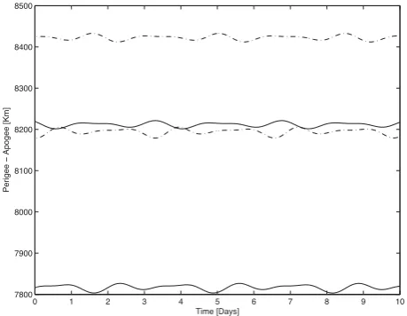
Figure 3. Evolution of the perigee (dashed line) and apogee (dash-dotted line) for a given couple of orbits as a function of time. There is an orbit crossing within 1 d of evolution.
of the entire population. Consequently, our filter I detects 21 730 false positives, which passed the first filter proposed by Hoots et al. (1984). Note that the main problem of the first filter presented by Hoots et al. (1984) was computing the ephemerides using the oscu-lating elements. This comparison has been done with our powerful interpolation ephemerides table instead of the osculating elements, even though our proposed filter I improves the filter of Hoots et al. (1984).
For clarity, Fig.2illustrates the geocentric distance of two objects, while Fig.3illustrates the evolution of the perigee and apogee of the same objects. In this particular case, we observe a false positive in the perigee–apogee criteria because, if we consider the geocentric distance of the pair of orbits, there is no risk approach, while if we consider the perigee–apogee criteria there is the possibility of an orbit crossing. Using these figures, we illustrate the efficiency of our filter I against that of Hoots et al. (1984).
4.3 Evolution of the distance function in filter II
Filter II uses the signed distance functions ˜d1 and ˜d2 presented
in equation (11), which represent the distances between two local
at University of Strathclyde on August 5, 2014
http://mnras.oxfordjournals.org/
[image:6.595.311.541.275.453.2]Figure 4. Evolution of the function ˜d1with a change of sign in the function, which implies that there is an orbit crossing.
Figure 5. Evolution of the function ˜d1 without a change of sign in the function, which implies that there is no orbit crossing.
minimal points. If one of the functions presents a change of sign, there is an orbit crossing; otherwise, there is not. Fig.4illustrates the evolution of the function ˜d1 when an orbit crossing occurs,
and consequently when a change of sign in the function is present. In this case, the first orbit crossing occurs within less than 1 d of propagation. Fig.5illustrates the evolution of the function ˜d1in
a pair of orbits where there is no orbit crossing, and consequently there is no change of sign in the function ˜d1.
4.4 Dependence of filter sequence on time-step
In this section, we apply the filter sequence to the same population of 864 pieces of space debris, but in this case, we consider a time-step of 0.008 d (≈12 min). The number of time nodes is now around 1300.
[image:7.595.316.543.93.137.2]Table1shows the number of pairs that pass the subsequent filters if we apply the filter sequence to the same population with different time-steps. We observe that the smaller the time-step is, the more accurate the results are, and consequently we can exclude more pairs at risk of collision. Note that when the time-step is 0.05, we obtain
Table 1. Pairs to be considered after applying each filter to a population of 864 pieces of space debris. Two different time-steps are used, and consequently the number of pairs that pass each filter changes.
dt=0.05 dt=0.008
Filter I Filter II Filer III Filter I Filer II Filer III
218 459 49 739 0 216 837 49 739 0
about 1622 false positives when applying filter I, which means that they are considered at real risk of collision, although they are not, because if we reduce the time-step, they are excluded. In the second filter, there are 256 false positives, and in the third filter, there are no false positives, because in both cases the number of pairs at real risk of collision is zero.
As can be seen, the more precision we need, the smaller the time-step needs to be. However, the smaller the time-time-step is, the more computational time is required. If we need a first approach, with certain feasibility, the time-step can be the biggest one. Thus, the computational time will be substantially reduced.
5 O R B I T U N C E RTA I N T Y
The only limitation of the filter sequence is the poor orbit deter-mination used to compute the ephemerides table. This poor orbit determination is a result of unannounced manoeuvres or a large ef-fect of drag perturbation. However, the uncertainty, so far not taken into account in this work, is also a problem. The uncertainty is the error produced when computing the locations of pieces of space debris in their orbits because of different observational errors. This means that each piece of space debris is associated with a covariance matrix indicating the quality of the computed position.
If we include the uncertainty of each object at each time in the ephemerides table, which is the probability of being exactly in that point at a given instant of time, we must use it in the filter sequence. Filter I can be improved by including the uncertainty in the calculation of the minimum and maximum distances, and then the method will be more realistic. Filter II can be improved by including the computation of the uncertainty on the signed distances, due to the uncertainty on the orbits. The property of differentiability of these functions at orbit crossing is now fundamental if one wants to apply a covariance propagation formula, requiring regularity, to compute a meaningful uncertainty for the distances.
6 C O N C L U S I O N S A N D F U T U R E W O R K
In this paper, we have focused on the avoidance of space debris collisions. To that end, we have designed a filter sequence that is able to disregard pairs of orbits that are not at real risk of collision. In detail, we have based the filter sequence on two procedures. The first procedure is the storage of the orbital ephemerides in a similar way as theSPICEkernels used by NASA, which allows easy
access to the data with a low RAM memory. The second procedure concerns three filters based on the mutual geometry of all pairs of orbits considered, and the time coincidence between them. We have applied this filter sequence to a population of 864 pieces of space debris, and we have compared our filter I with the one presented by Hoots et al. (1984) to prove the efficiency of our methodology. We have also analysed the influence of the time-step applied in the filter sequence, and we have discussed the results obtained.
As future work, we aim to consider some improvements of the filter sequence. First, there are cases in which the computation
at University of Strathclyde on August 5, 2014
http://mnras.oxfordjournals.org/
[image:7.595.51.282.290.471.2]of the minimum distance fails, coinciding with cases where the tangent vectors are parallel. Secondly, the time required is too long, and consequently some parallelization techniques can be applied. Finally, the ephemerides table can be computed more precisely (e.g. by including the atmospheric drag).
There are two different ways to continue this work. The first way is to consider more than 864 pieces of space debris (e.g. the approx-imately 21 000 objects that comprise the TLE catalogue), with their uncertainties, and to include the uncertainty in the functions of the filter sequence in order to compute pairs of objects at real risk of collision. The second way is to consider the TLE catalogue without orbit uncertainty, and to use the filter sequence proposed in this work for the entire catalogue of space debris. The increase of the computational cost can be reduced by applying some parallelization techniques.
AC K N OW L E D G E M E N T S
This paper presents the research results of the Belgian Network Dynamical Systems, Control, and Optimization (DYSCO), funded by the Interuniversity Attraction Poles Programme, initiated by the Belgian State, Science Policy Office. The scientific responsibility rests with its author(s). The authors would especially like to thank Giovanni F. Gronchi, who agreed to review this work.
R E F E R E N C E S
Acton C. H., 1996, Planet Space Sci., 44, 65
Broucke R. A., Cefola P. J., 1972, Celestial Mech., 5, 303
Casanova D., Lemaˆıtre A., 2014, Celest. Mech. Dyn. Astron., submitted
Delsate N., Lemaˆıtre A., Carletti T., Robutel P., 2010, Celest. Mech. Dyn. Astron., 108, 275
Dimare L., Farnocchia D., Gronchi G. F., Milani A., Bernardi F., Rossi A., 2011, in Ryan S., ed., Advanced Maui Optical and Space Surveillance Technologies Conference. Maui Economic Development Board, Maui, E51
Gronchi G. F., 2002, SIAM Journal on Scientific Computing, 24, 61 Gronchi G. F., 2005, Celest. Mech. Dyn. Astron., 93, 295
Gronchi G., Tommei G., 2007, Discrete and Continuous Dynamical Systems, Series B, 7, 755
Gronchi G. F., Tommei G., Milani A., 2006, in Valsecchi G. B., Vokrouh-lick´y D., Milani A., eds, Proc. IAU Symp. 236, Near Earth Objects, Our Celestial Neighbors: Opportunity and Risk. Cambridge Univ. Press, Cambridge, p. 3
Gronchi G. F., Dimare L., Milani A., 2010, Celest. Mech. Dyn. Astron., 107, 299
Hoots F. R., Crawford L. L., Roehrich R. L., 1984, Celest. Mech., 33, 143 Hubaux C., Lemaˆıtre A., Delsate N., Carletti T., 2012, Adv. Space Res., 49,
1472
Lemaˆıtre A., Delsate N., Valk S., 2009, Celest. Mech. Dyn. Astron., 104, 383
Milani A., Tommei G., Chesley S., Sansaturio M., Valsecchi G., 2005, Icarus, 173, 362
Pardini C., Anselmo L., 2011, Adv. Space Res., 48, 557
Valk S., Lemaˆıtre A., Anselmo L., 2008, Adv. Space Res., 41, 1077 Valk S., Lemaˆıtre A., Deleflie F., 2009a, Adv. Space Res., 43, 1070 Valk S., Delsate N., Lemaˆıtre A., Carletti T., 2009b, Adv. Space Res., 43,
1509
Woodburn J., Coppola V., Stoner F., 2010, Adv. Astronaut. Sci., 135, 1157
This paper has been typeset from a TEX/LATEX file prepared by the author.
at University of Strathclyde on August 5, 2014
http://mnras.oxfordjournals.org/