Low thrust propulsion in a coplanar circular restricted four body problem

(will be inserted by the editor)

Low-thrust propulsion in a coplanar circular restricted

four body problem

Marta Ceccaroni · James Biggs

Received: date / Accepted: date

Abstract This paper formulates a circular restricted four body problem (CRFBP), where the three primaries are set in the stable Lagrangian equilateral triangle con-figuration and the fourth body is massless. The analysis of this autonomous coplanar CRFBP is undertaken, which identifies eight natural equilibria; four of which are close to the smaller body, two stable and two unstable, when considering the primaries to be the Sun and two smaller bodies of the solar system. Following this, the model incor-porates ‘near term’ low-thrust propulsion capabilities to generate surfaces of artificial equilibrium points close to the smaller primary, both in and out of the plane containing the celestial bodies. A stability analysis of these points is carried out and a stable sub-set of them is identified. Throughout the analysis the Sun-Jupiter-Asteroid-Spacecraft system is used, for conceivable masses of a hypothetical asteroid set at the libration point L4. It is shown that eight bounded orbits exist, which can be maintained with a constant thrust less than 1.5×10−4Nfor a 1000kg spacecraft. This illustrates that, by exploiting low-thrust technologies, it would be possible to maintain an observation point more than 66% closer to the asteroid than that of a stable natural equilibrium point. The analysis then focusses on a major Jupiter Trojan: the 624-Hektor aster-oid. The thrust required to enable close asteroid observation is determined in the simplified CRFBP model. Finally, a numerical simulation of the real Sun-Jupiter-624 Hektor-Spacecraft is undertaken, which tests the validity of the stability analysis of the simplified model.

Keywords Restricted Problems·Stability·Periodic Orbits

Marta Ceccaroni

Advanced Space Concepts Laboratory University of Strathclyde, Glasgow, UK E-mail: [email protected] James Biggs

1 Introduction

The general, spatial, four body problem is a complex 24 degree of freedom system. However, the system can be reduced by exploiting integrals of motion to obtain a 12 degree of freedom system but cannot be reduced further without loss of generality. Fur-thermore, it is well known that with four (or more) massive bodies there is no analytical stability criterion valid for all time (Steves et al., 1998b). Therefore, the analysis of such “non-restricted” models have mainly been limited to finding some stability crite-rion relative to a particular configuration. Examples include Milani and Nobili (1983), on a four body linear hierarchical1system, and Roy et al. (1985), on fictitious coplanar four body systems with different distribution of masses and hierarchies, in which a numerical estimation of the duration of the stability for these systems is found. In or-der to or-derive stability properties over infinite time intervals, it is necessary to consior-der suitably simplified four body systems (Roy et al., 1985).

Examples of these “suitably simplified” models include autonomous configura-tions (given by the relative equilibrium soluconfigura-tions) such as the straight line (Multon, 1910), square, equilateral triangle and kite configurations (Multon (1900), Steves et al. (1998b), Pina and Lonngi (2009) and Sicardy (2011)), and non-autonomous models, such as the Caledonian Problem (namely the coplanar, initially circular, equal masses, four body problem), by Steves et al. (1998a). The latter is an important special case as, although it does not admit the Jacobi integral, it allows almost all the other con-ventional dynamical systems strategies to study the evolution and the stability of the trajectories (e.g. the identification of periodic orbits, the study of the linear stability (Hadjidemetriou, 1978) or the long term symplectic integration of the equations of mo-tion). Another class of simplified cases fall into the category of the “restricted” FBPs where one of the four bodies is considered massless. A study of relative equilibria in re-stricted FBPs can be found in Simo’ (1978). Furthermore, relative equilibrium solutions have been obtained in the special cases of equal mass symmetric configurations (e.g. the collinear symmetric CRFBP by Michalodimitrakis (1981)) or by using Hill’s approxi-mation (where the fourth body is assumed to be at a great distance and therefore its influence is reduced to a perturbing term, transforming the system into a perturbed re-stricted three body problem). Examples include Scheeres (1998) and Papadakis (2007), the bicircular (Cronin et al. (1964), Koon et al. (2008)), or the quasi-bicircular (Gomez et al., 2001) and the concentric circular models (Andreu, 2002). Among which papers (Gomez et al., 2001) and (Andreu, 2002) which use this model as an approximation to the Sun-Earth-Moon-Spacecraft system, highlight the lack of regions of “good stability properties” in the vicinity of the triangular lagrangian points of the smaller, perturbed system.

This paper investigates a particular restricted FBP, namely an autonomous (in a rotating frame) coplanar CRFBP, where the three massive bodies are set in the stable Lagrangian equilateral triangle configuration. This system, although dealing with the dynamics of three masses and a particle, is different from the previously mentioned restricted cases as it does not use Hill’s approximation or the assumption of equal mass and symmetric configurations. There does exist a number of studies on restricted FBP set in such a configuration mainly used to model existing binary systems (see

1 _{a system is said to be hierarchical if at a given epoch it can be defined to exist as a clearly}

Kloppenborg et al. (2010), Melita et al. (2008), Van Hamme and Wilson (1986), and Schwarz et al. (2009)). Of particular relevance are the papers by Alvarez-Ramirez and Vidal (2009) and Baltagiannis and Papadakis (2011) where the latter uses a numerical approach to determine the number of equilibrium points and a linear stability analysis depending on the distribution of the masses.

The objective of this paper is to identify completely novel orbits both for mathemat-ical interest as well as for potential future mission applications. Initially the natural evolution of this model is studied, which identifies eight natural equilibrium points; four of which are close to the asteroid. Following this, the system is perturbed by the inclusion of low-thrust propulsion (such as solar electric propulsion (SEP)) previously only considered in two and three-body restricted problems.

Space mission design for low-thrust spacecraft has been extensively investigated from the late 1990’s. So far the two major types of low-thrust propulsion, which have been studied in this context, are solar sails and SEP, the latter considered in this pa-per. Research on this topic, at present, mainly focus on finding artificial equilibria as in Morimoto et al. (2007), McInnes et al. (1994) and Baig and McInnes (2008), on generating non-Keplerian periodic orbits using solar sails or low thrust, e.g. Morimoto et al. (2006), Waters and McInnes (2007), Baig and McInnes (2009) and McKay et al. (2011), on the systematic cataloguing of non-Keplerian orbits using SEP as in McKay et al. (2009), or on analyzing the stability properties of minimum-control artificial equi-librium points as in Morimoto et al. (2007) and Bombardelli and Pelaez (2011), all of which are set in restricted two or three body models.

Throughout the paper the low-thrust Sun-Jupiter-Asteroid-Spacecraft is analyzed, as a particular case, for a range of estimated masses of a hypothetical Asteroid set to be trapped at the Lagrangian pointL4. Surfaces of artificial equilibrium points are then identified and a stability analysis of them undertaken. This paper highlights the poten-tial of this investigation for designing observation missions to the Jupiter Trojans. This swarm of asteroids has been recognized as a present target for space science missions, as understanding it may lead to clues to the origin and dynamical evolution of Jupiter itself (Shoemaker et al., 1988). Currently, the Trojan asteroids are completely unex-plored and largely unknown and any visit by a spacecraft will revolutionize our current understanding of these bodies (Rivkin et al., 2009). Moreover, although moving on tadpole orbits around theL4andL5 points of the Sun-Jupiter-Spacecraft system (see Marzari (2006)), these asteroids are often modeled as fixed in the equilateral triangle configuration, e.g. considering them as concentrated atL4, (see Marzari et al. (2002), Steves et al. (1998b), Steves et al. (1998a)). This configuration is also considered as the Solar system example of the equilateral triangle relative equilibrium solution found by Lagrange (Dvorak et al. (2008) and Baltagiannis and Papadakis (2011).

2 The autonomous coplanar CRFBP

In this paper an autonomous coplanar CRFBP is analyzed; it is the problem of deter-mining the dynamics of a bodyPS that moves under the influence of the gravitational field generated by three massive bodies,Pj of massesmj, j= 1,2,3 respectively (say

m1≥m2≥m3). It is called restricted as the bodyPS is assumed to have negligible mass mS = 0. Furthermore it is Coplanar and circular since all the massive bodies revolve in the same plane and with the same angular velocity ω, following circular orbits around the barycenter ofP1andP2.

Finally, it is autonomous as, taking a rotating frame of referenceOx,y,z, where thex/y plane contains the three bodies, centered in the center of rotation of the planets and revolving around the third axis with the same angular velocityωof the bodies, all the primariesP1,P2andP3will be fixed in the rotating frame.

Moreover, in this paper, the primaries are set in the Lagrangian equilateral triangle configuration where the position of the third primary P3 corresponds to one of the triangular Lagrangian points, such that the three massive bodies form an equilateral triangle, as in Ambrosetti and Prodi (1993).

This configuration is well known to be stable if the masses of the three planets satisfy the condition m1m2+m1m3+m2m3

(m1+m2+m3)2 < 1

27 (see Gascheau (1843) , Routh (1875), Erdi et al. (2009) and Schwarz et al. (2009)); this condition is equivalent to 27(m1m2+

m1m3+m2m3)−(m1+m2+m3)2<0.

As we assumed m3 ≤ m2 and the left term of this inequality is monotonically increasing in m3, ∀m3 ∈ (0, m2), such left term is maximized for m3 = m2, thus: 27(m1m2+m1m3+m2m3)−(m1+m2+m3)2<27(2m1m2+m22)−(m1+ 2m2)2

∀m1, m2.

Therefore the stability condition becomes:−m2₁+50m1m2+23m22<0 (more restrictive then the previous), that rearranged is: m1

m2 >25 + 18

√

2. In addition, the mass of the Asteroid is taken to be small enough not to influence the motion of the main primaries

P1 andP2 (i.e. the center of rotation of the system remains in the barycenter of the two main bodies).

Scaled units of measure for mass and distance are used, normalized with the sum of the masses ofP1andP2and their distance respectively, while the gravitational constant

Gand the rotational velocityωof the system are set to 1. In nondimensional units let

µ, 1−µandbe the scaled mass of P2,P1 andP3 respectively, whereµ= m1m+m2 2,

1−µ= m1 m1+m2,=

m3

m1+m2 andm3m1, m2.

As the system of reference has its origin in the barycenterOand it rotates with the same angular velocity ofP1andP2, these two planets will be fixed and, without loss of generality, we can consider their positions to beP1= (−µ,0,0), P2= (1−µ,0,0).This implies that, in order to form an equilateral triangle with them, the position of the third primary has to be:P3= (Lx, Ly,0) = (1₂−µ,

√

3

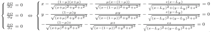
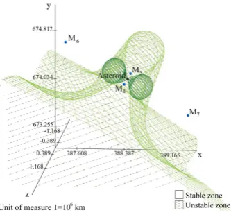
2 ,0).The system just described is shown in Figure 1.

The dynamics of the massless spacecraft, whose state vector is expressed in non-dimensional cartesian coordinatesx= [x, y, z, vx, vy, vz]T, is described by the system:

 

 ¨

x= 2 ˙y−∂Ω_∂x ¨

y=−2 ˙x−∂Ω_∂y ¨

z=−∂Ω ∂z

Fig. 1 The autonomous coplanar CRFBP;in a rotating frame of reference, the planets are fixed and form an equilateral triangle

where the augmented or effective potential and the distances of the spacecraft from each of the three primaries are respectively:

Ω=−x2+y₂ 2−(1_r−µ)

1 − µ r2 −

r3,

r1= p

(x+µ)2_+y2_+z2_,

r2= p

(x+µ−1)2_+y2_+z2_,

r3= p

(x−Lx)2+ (y−Ly)2+z2,

and ∂Ω_∂x, ∂Ω_∂y and ∂Ω_∂z are the partial derivative ofΩwith respect tox,yandz, while the “dot” symbolizes differentiation with respect to time.

Note that if→0, system (1) degenerates to the classical CR3BP, while if both→0 andµ→0 it becomes a R2BP.

In order to find the equilibrium points of the system, the velocities ˙x, y,˙ z˙and the accelerations ¨x, y,¨ z¨are set to be zero in (1) obtaining:

           ∂Ω ∂x = 0 ∂Ω ∂y = 0 ∂Ω ∂z = 0

⇔             

x−√ (1−µ)(x+µ)

(x+µ)2 +y2 +z2 3

−√ µ(x−(1−µ))

(x−(1−µ))2 +y2 +z2 3

−q (x−Lx)

(x−Lx)2 +(y−Ly)2 +z23 = 0 y−√ (1−µ)y

(x+µ)2 +y2 +z2 3

−_√ µy

(x−(1−µ))2 +y2 +z2 3

−q (y−Ly)

(x−Lx)2 +(y−Ly)2 +z23 = 0

−√ (1−µ)z

(x+µ)2 +y2 +z2 3 −

µz √

(x−(1−µ))2 +y2 +z2 3−

z q

(x−Lx)2 +(y−Ly)2 +z23 = 0 (2) As we are in the stable Lagrangian configuration such system admits eight solutions (see Baltagiannis and Papadakis (2011)), the equilibrium pointsMj, j= 1, ...,8, de-fined at the intersections of the three surfaces described by its equations, see Appendix A.

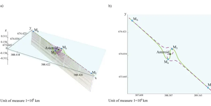
Figures 2 and 3 show the behavior of the three surfaces which satisfy system (2) in the vicinity of the third primary; in this region such surfaces form four equilibrium points M4,M5, M6 and M7 on which this paper is focussed. The former shows the three surfaces in three dimensions, while the latter represents them sectioned by the

z= 0 plane, part a), and intersected with this plane, part b).

show the solution of ∂Ω_∂y = 0, while the solution of the third equation is the plane

z = 0, plotted in the Figures as well. As the third equation is satisfied by the plane

z= 0, all the equilibria are bounded to stay on this plane, which, equivalently, can be seen as the degeneration of system (2) into a two dimensional system forz = 0 (see Ceccaroni and Biggs (2010)).

Fig. 2 The four equilibria close to the asteroid;spatial view

Fig. 3 The four equilibria close to the asteroid; a) z = 0 section of the spatial view; b)

Intersection with the planez= 0

as shown in the Figure 4 a) and b) where the first shows the behavior of the four equilibrium points as the mass of the asteroid increases while the second is focussed just onM4andM5.

Thus, we would conclude that the only assumptions on the masses of our sys-tem should be the stability condition, which, in nondimensional units, becomes: µ <

(13−9√2)

14 and that the mass of the asteroid has to be small enough such that it does not affect the motion of the other two Primaries.

Fig. 4 Equilibrium Points; a) ∀∈(0, µ)the two lines intersects four times in the region near the asteroid; b)Zoomed image

3 Stability analysis

Hereafter, for simplicity of notation, (xe, ye, ze) will indicate a generic equilibrium so-lution of system (2); moreover, for convenience, a translation to a generic equilibrium point (xe, ye, ze) is performed:

 



x0=x−xe

y0=y−ye

z0=z−ze

(3)

but, to simplify notation, we will ignore the indices abovex0, y0, z0.

Then we linearize the motion close to this generic point (xe, ye, ze), obtaining

       

       ˙

x=vx ˙

y=vy ˙

z=vz ˙

vx= 2vy+αx+χy+δz ˙

vy=−2vx+χx+βy+φz ˙

vz=δx+φy+γz

with

α= 1 +(1−µ)

h

2(xE+µ)2−_yE2−_zE2i q

(xE+µ)2 +y2

E+z2E

5 +

µ h

2(xE+µ−1)2−_yE2−_zE2i q

(xE+µ−1)2 +y2

E+z2E

5 +

h

2(xE−Lx)2−(_yE−Ly)2−_zE2i q

(xE−Lx)2 +(yE−Ly)2 +z2

E

5 , β= 1 +(1−µ)

h

−(_xE+µ)2 +2yE2−z_E2 i

q

(xE+µ)2 +y2

E+z2E

5 +

µ h

−(_xE+µ−1)2 +2_yE2−z_E2 i

q

(xE+µ−1)2 +y2

E+z2E

5 +

h

−(_xE−Lx)2 +2(yE−Ly)2−z_E2 i

q

(xE−Lx)2 +(yE−Ly)2 +z2

E

5 , γ=(1−µ)

h

−(_xE+µ)2−_yE2 +2z_E2 i

q

(xE+µ)2 +y2

E+z2E

5 +

µ h

−(_xE+µ−1)2−_yE2 +2z2_E i

q

(xE+µ−1)2 +y2

E+z2E

5 +

h

−(_xE−Lx)2−(_yE−Ly)2 +2z_E2 i

q

(xE−Lx)2 +(yE−Ly)2 +z2

E

5 , χ= 3

(

(1−µ)[(xE+µ)yE]

q

(xE+µ)2 +y2_E+z2_E5

+q µ[(xE+µ−1)yE]

(xE+µ−1)2 +y2_E+z2_E5

+q [(xE−Lx)(yE−Ly)]

(xE−Lx)2 +(yE−Ly)2 +z2_E5

) ,

δ= 3 (

(1−µ)[(xE+µ)zE]

q

(xE+µ)2 +y2_E+z2_E5

+q µ[(xE+µ−1)zE]

(xE+µ−1)2 +y2_E+z_E25

+q [(xE−Lx)zE]

(xE−Lx)2 +(yE−Ly)2 +z_E25

) ,

φ= 3 (

(1−µ)[yE zE]

q

(xE+µ)2 +y2

E+zE2

5+

µ[yE zE]

q

(xE+µ−1)2 +y2

E+z2E

5 +

[(yE−Ly)zE]

q

(xE−Lx)2 +(yE−Ly)2 +z2

E

5

) .

(5)

CallingAthe matrix corresponding to system (4), namely:

A=        

0 0 0 1 0 0 0 0 0 0 1 0 0 0 0 0 0 1

α χ δ 0 2 0

χ β φ−2 0 0

δ φ γ0 0 0         (6)

The characteristic polynomial ofAis

Ψ6+ (4−α−β−γ)Ψ4+ (αβ+αγ+βγ−χ2−δ2−φ2−4γ)Ψ2+ (αφ2+βδ2

+γχ2−αβγ−2χδφ) = 0.

(7) As (7) is a biquadratic equation it is useful to setΓ =Ψ2, and, observing that (4−

α−β−γ) = 2 in (5), yields the monic polynomial of the third degree:

Γ3+ 2Γ2+ (αβ+αγ+βγ−χ2−δ2−φ2−4γ)Γ+ (αφ2+βδ2+γχ2−αβγ

−2χδφ) = 0. (8)

Following the usual procedure to solve third degree polynomials, see for example, Artin (1991), we call

p=−4₃+ (αβ+αγ+βγ−χ2−δ2−φ2−4γ),

q=16₂₇−2(αβ+αγ+βγ−₃χ2−δ2−φ2−4γ)+ (αφ2+βδ2+γχ2−αβγ−2χδφ), ∆=q₄2+p₂₇3.

(9)

Then it is well known that the three solutions Γ1,2,3 of (8) are the only three solutions among those nine

Γ1,2,3= 3 q

−q₃+√∆+q3 ₋q 3−

√

∆−2

3 (10)

such as

3

q

−q₂+√∆

·

3

q

−q₂−√∆

This means that the six eigenvalues of system (4) will beΨk, k= 1, ...,6 defined as:

Ψk=± p

Γj k= 1, ...,6; j= 1,2,3. (12)

By the stability result for unequal masses of Baltagiannis and Papadakis (2011), there exist a lower limit for the mass ratio m1

m1+m2(= 1−µ) such as, for all the values

bigger than that, the pointsM6andM7are always stable, which happens, for example, when fixing the three massive bodies in our model to be the Sun and any other two objects of the Solar System. Moreover, as such ratio decreases with the increase in mass of the second primary, we fix m1

m1+m2 to be the minimal obtainable for the solar system,

or, equivalently, we chooseP2to be Jupiter (i.e.µ= 0.000953592, 1−µ= 0.999046), configuration that, in particular, satisfies the stability condition (1−_µµ) >25 + 18√2 that can also be rearranged as:µ <(13−9

√

2) 14 .

From now on, we will consider the main primaries of our system to be the Sun and Jupiter; therefore, fixing a specific mass ∈(0, µ) for the hypothetical asteroid, and evaluating the eigenvalues corresponding to both the equilibrium pointsM4and M5, the∆will be negative, while√−3pwill be greater than one, which, as will be shown later on, means that at least one of the three eigenvalues will have Real part non-zero, i.e. the equilibrium points are linearly unstable and therefore nonlinearly unstable; on the other hand for both the equilibrium pointsM6andM7, the∆will be negative, and

√

−3pwill be smaller than one, which, implies that all the eigenvalues will be purely imaginary, i.e. the equilibrium points are linearly stable.

4 The low-thrust autonomous coplanar CRFBP

The dynamics of a low-thrust spacecraft in the autonomous coplanar CRFBP is now in-vestigated. Using SEP propulsion our spacecraft can create artificial equilibrium points in the spatial vicinity of the asteroid, suitable for observation missions. In addition, a subset of these novel equilibrium points are proved to be stable, such that the motion will remain bounded in a small region about them, with relatively low fuel requirements and without the need for a state feedback control.

Given a maximum thrust capability Fmax, expressed in N, and an approximate weight for the spacecraft Ws, evaluated inkg, the maximal acceleration in the non-dimensional units is given by:

amax= F_Wmax

s

N kg =

Fmax

Ws ·

m s2

= Fmax_W

s ·

Kg m2

m3 Kg·s2

= Fmax_W

s

d2

P1/P2 (m1+m2)

1

G,

(13)

whered_P1/P2 means the distance in meters between the two major Primaries. The acceleration will be indicated withanˆ=ax¯x+ayy¯+az¯z, whereax,ay, andaz are the components of the acceleration in thex,yandzdirections,a=pa2x+a2y+a2z is the magnitude and ˆnis the direction of the acceleration itself.

the maximum accelerationamax(corresponding to the maximal thrustFmax= 0.3N) will therefore be 1.36765. Moreover the acceleration has to be constant in the direction of the perturbation, namely

∂ ∂x(anˆ) =

∂ ∂y(anˆ) =

∂

∂z(anˆ) = 0. (14)

Adding low-thrust to system (1) it becomes:

 

 ¨

x= 2 ˙y−∂Ω_∂x +ax ¨

y=−2 ˙x−∂Ω_∂y +ay ¨

z=−∂Ω_∂z +az

(15)

withΩ,a,r1,r2andr3as in (1).

Again, to find the equilibrium points, the velocities ˙x,y,˙ z˙and the accelerations ¨x, y,¨ ¨z

are set to be zero in (15), obtaining:

 



ax=∂Ω_∂x

ay=∂Ω_∂y

az= ∂Ω_∂z

⇔  



a=|∇Ω|

ˆ

n=−_|∇∇Ω_Ω|

(16)

In which, the second system states that, in order to get a new equilibrium point, the acceleration on the spacecraft due to the thrusters has to be equal in magnitude (first equation) but opposite in direction (second equation) to the acceleration on the spacecraft due to the gravitational field at that point; the sign of the three compo-nentsax,ay andaz will therefore be determined (and, in particular, opposite) by the respective components of the gravitational field evaluated in the point.

5 Stability analysis of the linearized system

Notice that, with a constant thrust, system (15), once linearized, is equal to the linear system in (4) and therefore the linear stability of the equilibrium points resulting from system (16) will be given by the analysis of the eigenvalues in (12). By the Lyapunov Stability theorem, see for example Arnold et al. (2006), in order to obtain a linearly bounded motion, the eigenvalues must have Real part less than or equal to zero. In our case, we cannot accept a non zero Real part, as it would imply that eitherRe(Ψ2k−1)> 0 or Re(Ψ2k) = Re(−Ψ2k−1) = −Re(Ψ2k−1) > 0 for k = 1 and/or 2 and/or 3 , and this would lead to a saddle×saddle×saddle, asaddle×saddle×center or a

saddle×center×center unstable equilibrium point.

Therefore, in this case, the only acceptable way to get a linearly bounded motion is withRe(Ψk) = 0,∀k= 1, ...,6.

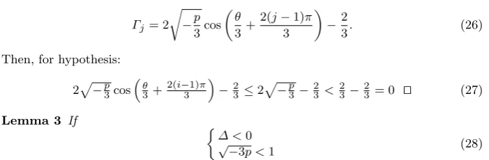
Lemma 1 If∆ <0then the solutionsΓj, j= 1,2,3of (8) are inR.

Proof: Let be∆ <0.

From (10) and (11), and considering the fact that∆ <0, the solutionsΓj, j= 1,2,3 of (8) can be rearranged to yield the three solutions among these nine

Γ1,2,3= 3 r

−q 3+i

√ −∆+ 3

r −q

3−i √

−∆−2

that satisfy the condition:

3

r −q

2+i √ −∆ · 3 r −q

2−i √

−∆

=−p

3∈R. (18)

Notice that, from system (9),

∆ <0⇒p <0 (19)

and that the two numbers

−q₂+i√−∆

−q₂−i√−∆ (20)

are complex conjugates (same Real part, opposite Imaginary part) such that:

| −₂q+i√−∆|=| −q₂−i√−∆|= q

(−q₂)2₋₍√_−∆)2₌p

−p₃ ∈R. (21)

Calling θ=    arctan −2 √ −∆ q

if q <0

arctan −2 √ −∆ q

−π if q >0

(22)

the two numbers can be rewritten as:

q

−p₂₇3(eiθ) q

−p₂₇3(e−iθ)

(23)

Thus, extracting the cubic root, gives:

p

−p₃(ei(θ3+2kπ3 )₎

p

−p₃(ei(−θ3+2hπ3 )₎

(24)

withh, k= 0,1,2.

For condition (18), we can only accept the couples (h= 0;k= 0), (h= 2;k= 1) and (h = 1;k = 2). This implies that our three acceptable solutions of (8) can be summarized in a compact form as:

Γj= p

−p₃(ei(θ3+ 2(j−1)π

3 )_+ei(−

θ

3+ 4(j−1)π

3 )₎−2 3 =p−p₃cos

θ 3+

2(j−1)π 3

+isin

θ 3+

2(j−1)π 3

+p−p₃cos

θ 3+

2(j−1)π 3

−isin

θ 3+

2(j−1)π 3

−2₃ = 2p−p₃cos

θ 3+

2(j−1)π 3

−2

3,

(25)

withj= 1,2,3.

Which demonstrates that∆ <0⇒Γj∈R, ∀j= 1,2,3ut.

Proof:

By (25) for eachj= 1,2,3 we can rewriteΓj as

Γj= 2 r

−p 3cos

θ

3+

2(j−1)π

3

−2

3. (26)

Then, for hypothesis:

2p−p₃cosθ₃+2(i−₃1)π−2₃ ≤2p−p₃−2₃< 2₃−2₃ = 0 ut (27)

Lemma 3 If

∆ <0 √

−3p <1 (28)

then the six eigenvalues of system (4) are purely Imaginary.

Proof:

The proof of the Lemma is straight forward since the eigenvalues of (4) are Ψk =

±p

Γj, k= 1, ...,6; j= 1,2,3. Considering the hypothesis and applying Lemma 1, indeed, yields thatΓ ∈R,∀j= 1,2,3. Then, for Lemma 2,Γj<0,∀j= 1,2,3, which are the two conditions that lead to the thesis of Lemma 3ut.

Therefore, the six eigenvalues can be rearranged in the form:

Ψk=±i p

−Γj, k= 1, ...,6; j= 1,2,3. (29)

Figure 5 shows the spatial view of the three possible topologies of the zone that satisfies the conditions in (28), obtained for a realistic range for the mass of the hypothetical asteroid (i.e. from zero to the total mass of the Jupiter Trojans∼6×1020kg).

In particular part a) of the Figure represents the topology of the “four leaf clover” (Ceccaroni and Biggs, 2010) form3 ∈[0; 1.648×1017[ (⇒∈ [0; 8.27632×10−14[), part b) represents it form3= 1.648×1017(⇒= 8.27632×10−14), and part c) for

m3∈]1.648×1017; 6×1020] (⇒∈]8.27632×10−14; 3.01356×10−10]).

Fig. 5 The possible topologies obtainable varying the mass of the Asteroid;a)m3∈[0; 1.648×

1017_{[ (⇒ ∈ [0; 8.27632×10}−14_{[). b) m}

For displaying purpose only, from now on, the mass of the Asteroid will be set to be equal to the major of the actual Trojan Asteroids, namely 624-Hektor, therefore fixing

m3= 1.4×1019kg (which implies= 7.03165×10−12). Qualitatively the results for this value will be the same as for each value in the range considered, from zero to the total mass of the Jupiter Trojans.

Fig. 6 Linearly stable/unstable zones;the three dimensional “four leaf clover” boundary be-tween the linearly stable and the unstable zones near the asteroid

Fig. 7 Linearly stable/unstable zones; a)z= 0 section of the spatial view;b)Intersection with the planez= 0

Figure 6 represents the spatial view of the linearly stable zone of the Sun-Jupiter-Asteroid-Spacecraft system, while, once again, Figure 7 represents the horizontalx/y

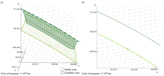
Of course, there exist an upper, external limit of the linearly stable zone as repre-sented in Figure 8.

Fig. 8 The outside boundary;The linearly stable zone is bounded.

Fig. 9 The outside boundary; a)z= 0 section of the spatial view b)Intersection with the planez= 0

With reference to Figure 5 we should note that the external limit is separated from the four leaf clover for small values of the mass of the asteroid, then approaches it as the mass of the Asteroid grows to 1.648×1017kg, where two surfaces becomes tangent, and finally, as the mass overcomes such value, the two surfaces merge together and the lower part of the four leaf clover opens.

The maximum possible thrust required to overcome the lower outside boundary is about 7×10−4N while for the upper one the thrust required is about 2.5×10−2N. However, for the system considered, the maximum thrust actually needed for this simplified model will be lower than 1.5×10−4N.

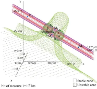
For the purpose of exposition, eight linearly stable artificial equilibrium pointsA, B, C, D, E, F, G, H are chosen, which have to fulfill three main requirements: to be generated by a thrust lower than 1.5×10−4N, to be at a distance from the unstable zone equal or higher than 3500km(far enough from the unstable zone to account for the likelihood of injection/position errors of the spacecraft), but remaining as close as possible to the asteroid. Moreover we take the first four lying on the x/y plane, while the other on the x0/z plane wherex0 is the tilted horizontal axis y = −(x−

Lx)M_M5₅x−M4x

y−M4y +Ly, (i.e. the line passing through the asteroid and perpendicular to the

segment connectingM4andM5). The eight points (whose coordinates are listed in the electronic supplementary material A (online only)) result to be at a distance smaller than 300000km from the asteroid (note that the distance of the stable equilibrium points from the Asteroid is about 1.16×106km, more that two thirds bigger than the distance of the asteroid from the artificial equilibrium points chosen).

In this system, in non-dimensional units, the amount of thrust required to create the two artificial points inA= (Ax;Ay;Az) and in G= (Gx;Gy;Gz) are evaluated; the behavior of the dynamics close to these two artificial equilibrium points, as well as their required thrust, are representative of the four points on thez = 0 plane, and for the four on thex0/z plane respectively, as can be seen in Figures 11 and 12, and, therefore, will be the only two investigated in detail.

To this end the computation of the gravitational field in bothAandGis needed:

                        

ax=−Ax+q (1−µ)(Ax+µ)

(Ax+µ)2 +A2_y+A2_z3

+q µ(Ax−(1−µ))

(Ax−(1−µ))2 +A2_y+A2_z3

+q (Ax−Lx)

(Ax−Lx)2 +(Ay−Ly)2 +A2

z

3 = 0.000233755

ay=−Ay+

(1−µ)Ay q

(Ax+µ)2 +A2_y+A2_z3

+q µAy

(Ax−(1−µ))2 +A2_y+A2_z3

+q (Ay−Ly)

(Ax−Lx)2 +(Ay−Ly)2 +A2

z

3 = 0.000521729

az=q (1−µ)Az

(Ax+µ)2 +A2_y+A2_z3

+ µAz

q

(Ax−(1−µ))2 +A2_y+A2_z3

+ Az

q

(Ax−Lx)2 +(Ay−Ly)2 +A2

z

3 = 0

(30)

which yields to a =pa2

x+a2y+a2z = 0.000571701 corresponding approximately to a force of 0.000125406N; the same evaluation for the pointGleads to (ax, ay, az) = (0.0000240703,−0.00001415,0.00034275) which is a=pa2x+a2y+a2z = 0.000343885 corresponding approximately to a force of 0.000075433N.

These thrusts are represented respectively by the two “tube shaped”, meshed sur-faces in Figures 10, 11 and 12; the first thrust is approximately the same required to create the other three equilibrium points lying on thex/yplane (B, C, andD), while the other is approximately the same required to create artificial equilibrium points set on thex0/z plane (E, F, and H). Figure 11 a) and b) represents the horizontal x/y

section and the intersection with thex/yplane of Figure 10.

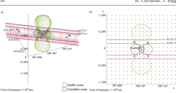
in terms of visual presentation, to section and intersect it with the vertical planex0/z

as shown in Figure 12 a) and b) respectively.

Note that, the eight points in Figures 10, 11 and 12 lie 3500kmoutside the linearly unstable zone, although it is not easy to visualize.

Fig. 10 Adding the low-thrust;eight artificial equilibrium points are created in the linearly stable zone using a thrust lower than1.5×10−4

Fig. 11 Adding the low-thrust; a)z= 0section of the spatial view;b)Intersection with the planez= 0and projection on this plane of the direction of the thrust required

Fig. 12 Adding the low-thrust; a)x0/z section of the spatial view;b)Intersection with the planex0/z and projection on this plane direction of the direction of the thrust required

6 Integrating the linearized motion Theorem 1 For a linear system of the form:

˙ x=Ax x(t0) =x0

(31)

wherex∈R6 and

A ∈ L(R6) := linear operatorsA:R6→R6, with real coefficients , ifAhas three couples of eigenvalues complex conjugated λ, λ∗;ν, ν∗;ϕ, ϕ∗ ∈ C, where the complex conjugated is indicated by the∗, such that:

λ=λ

R+iλI, ν=ν

R+iνI, ϕ=ϕ_R+iϕ_I,

(32)

where λR = Re(λ) and λI = Im(λ) and λ_I, ν_I, ϕ_I 6= 0; then there exist a base of

vectors {u1,w1,u3,w3,u5,w5}, with u2j−1,w2j−1 ∈ R6 ∀j= 1,2,3, and where

f2j−1=u2j−1+iw2j−1, j= 1,2,3are the eigenvectors of system (31), such that, in

this basis, the solution_ג(t) = [ξ1(t), ξ2(t), ψ1(t), ψ2(t), ζ1(t), ζ2(t)]T of the problem is: 

      

      

ξ1(t) =eλRt cos (λ_It)ξ10+ sin (λIt)ξ

0 2

ξ2(t) =eλRt cos (λ_It)ξ20−sin (λIt)ξ

0 1

ψ1(t) =eνRt cos (ν_It)ψ01+ sin (νIt)ψ

0 2

ψ2(t) =eνRt cos (ν_It)ψ02−sin (νIt)ψ

0 1

ζ1(t) =eϕRt cos (ϕ_It)ζ10+ sin (ϕIt)ζ

0 2

ζ2(t) =eϕRt cos (ϕIt)ζ02−sin (ϕIt)ζ

0 1

(33)

And therefore the solutionx(t) = [x(t), y(t), z(t), vx(t), vy(t), vz(t)]T of system (31) will

be x(t) = Mג(t) where Mis the matrix which provide the expression of the original

coordinatesx= [x, y, z, vx, vy, vz]T in terms of the new one,ג= [ξ1, ξ2, ψ1, ψ2, ζ1, ζ2]T,

Proof:

The proof of this theorem is given in Appendix B.

For the theorem above it is enough to find the eigenvectors of the system, and its solutions will be automatically obtained; moreover it will also provide the matrixM of the change of coordinates, as will be shown later on.

The eigenvalues of the system will be the six vectorsfj=uj+iwj∈C6, j= 1, ...,6 which solve

Afj=Ψjfj, j= 1, ...,6. (34)

As the six eigenvalues are three couples of complex conjugated numbers, the eigenvec-tors must be three couples of complex conjugated veceigenvec-tors, namelyf2j=u2j+iw2j= u2j−1−iw2j−1=f2j∗−1, ∀j= 1,2,3. This, in particular implies that it is sufficient to find three of the six eigenvectors, i.e.f1, f3andf5. Moreover, in the case considered in this paper, the eigenvalues have null Real part (i.e. are purely imaginary), and can therefore be stated in a simpler form.

Therefore, to simplify notation, hereafter the eigenvectors of the system will be:

Ψ1=λi,

Ψ2=−λi,

Ψ3=νi,

Ψ4=−νi,

Ψ5=ϕi,

Ψ6=−ϕi.

(35)

A few algebraic manipulations of (34) lead to the determination of the coefficients

uk,j k = 1,3,5 j = 1, ...,6 of the three eigenvectors corresponding to the eigenval-uesλi, νi, ϕirespectively; these coefficients are listed in the supplementary electronic material B.

Than the matrixM=

Mj,k

j= 1, ...,6

k= 1, ...,6

of the change of coordinates will be given

by

Mj,k=

uk,j ifk odd

wk−1,j ifkeven

(36)

Applying the transformation of coordinatesM−1onx= [x, y, z, vx, vy, vz]T, yields the new coordinates_ג= [ξ1, ξ2, ψ1, ψ2, ζ1, ζ2]T, namely:

ג=M−1x. (37)

The transformationM−1is then performed on the system (4) to find it’s expression in the new coordinates:

˙

ג=M−1x˙=M−1Ax=M−1A Mג. (38) Such a system can be rewritten as:

˙

ג=A0 ג with A0=M−1A M (39) with

A0= 

      

0 λ0 0 0 0

−λ0 0 0 0 0

0 0 0 ν0 0

0 0 −ν0 0 0

0 0 0 0 0 ϕ

0 0 0 0−ϕ0 

      

whose solutions are               

ξ1(t) = cos (λt)ξ10+ sin (λt)ξ02

ξ2(t) = cos (λt)ξ20−sin (λt)ξ01

ψ1(t) = cos (νt)ψ01+ sin (νt)ψ02

ψ2(t) = cos (νt)ψ02−sin (νt)ψ01

ζ1(t) = cos (ϕt)ζ10+ sin (ϕt)ζ20

ζ2(t) = cos (ϕt)ζ20−sin (ϕt)ζ10

(41)

Therefore the solution of system (15), given byx(t) =Mג(t), are:

            

x(t) =M1,1ξ1(t) +M1,2ξ2(t) +M1,3ψ1(t) +M1,4ψ2(t) +M1,5ζ1(t) +M1,6ζ2(t) =u1,1ξ1(t) +w1,1ξ2(t) +u3,1ψ1(t) +w3,1ψ2(t) +u5,1ζ1(t) +w5,1ζ2(t) y(t) =M2,1ξ1(t) +M2,2ξ2(t) +M2,3ψ1(t) +M2,4ψ2(t) +M2,5ζ1(t) +M2,6ζ2(t)

=u1,2ξ1(t) +w1,2ξ2(t) +u3,2ψ1(t) +w3,2ψ2(t) +u5,2ζ1(t) +w5,2ζ2(t) z(t) =M3,1ξ1(t) +M3,2ξ2(t) +M3,3ψ1(t) +M3,4ψ2(t) +M3,5ζ1(t) +M3,6ζ2(t)

=u1,3ξ1(t) +w1,3ξ2(t) +u3,3ψ1(t) +w3,3ψ2(t) +u5,3ζ1(t) +w5,3ζ2(t)

(42)

where the coefficientsuk,j k= 1,3,5 j= 1, ...,6 are listed in the electronic supple-mentary material B.

Notice that, evaluatingx(0) = [x(0), y(0), z(0),x˙(0),y˙(0),z˙(0)]T, as expected, yields:

        x(0) y(0) z(0)

vx(0)

vy(0)

vz(0)         =M        

ξ₁0 ξ20

ψ10

ψ₂0 ζ10

ζ₂0

        (43)

which is equal to (37) evaluated att= 0.

Recall that these resulting orbits, solutions of the linearized system, are expressed in the system of reference translated to the artificial equilibrium point xe, ye, ze(see (3)) such that they must be translated back to the barycenter ofP1 andP2.

As the behaviors of the linear solution in (42), in the vicinity of the pointsAand

G, is qualitatively the same as the other six artificial equilibria, the dynamics starting sufficiently close to these two points is shown, for the Sun-Jupiter-Asteroid-Spacecraft system, where the spacecraft has the same mass of 624-Hektor, in Figures 13 and 14.

In these Figures, thex/y,x/zprojections of the solution of the linearized system are represented by the dark, continuous lines. As expected, after 12 Jovian years (∼ 150 Earth years), they are still close to the respective starting points.

The dashed projection of the 3500km spherical domains around the points are also plotted in the Figures.

Notice that, if the perturbation (the position error) on thezaxis was null, the orbit starting close to the pointAwould qualitatively degenerate to the two dimensional case analyzed in Ceccaroni and Biggs (2010).

7 Integrating the full nonlinear system

Fig. 13 The solution of the linearized system in the vicinity of the pointAafter 12 Jovian years;a)x/yprojection; b)x/z projection

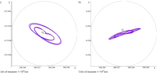
Fig. 14 The solution of the linearized system in the vicinity of the pointGafter 12 Jovian years;a)x/yprojection; b)x/z projection

Recalling the evaluation of the thrust needed to create artificial equilibrium points in

AandGstated in Section 5, a numerical integration with Mathematica using a Runge-Kutta method is performed, starting sufficiently close to our initial points. The dark, continuous lines in Figures 15 and 16 are thex/yandx/zprojections of the numerical solutions close toAandGrespectively, evaluated for a null initial velocity. Once again the solutions are represented for the first 12 Jovian years and the dashed projection of the 3500kmspherical domains around the points appears in the Figures as well.

Fig. 15 The solution of the full nonlinear system in the vicinity of the pointAafter 12 Jovian years;a)x/yprojection; b)x/z projection

Fig. 16 The solution of the full nonlinear system in the vicinity of the pointGafter 12 Jovian years;a)x/yprojection; b)x/z projection

conditions as there is a trade-off between the amplitude of the oscillations about the initial point (in the z direction) and the fuel required, i.e. fuel can be saved at the expense of larger oscillations.

8 The numerical simulation of the real system

plane will greatly affect the change of velocity of the system ˙ω(in the theoretical model ˙

ω= 0) therefore representing the main difference between the two models.

The eight artificial equilibria chosen in Section 6, which are bounded in the simplified model, in the real model result to be unstable, quickly diverging from 624-Hektor. The

x/yprojections of their orbits are shown in Figure 17 for a period of around 36 years (∼3 revolutions of Jupiter(and of Hektor) around the Sun).

The numerical integration of many other artificial equilibrium points was then

under-Fig. 17 The unstable zone of the model enlarges and the eight artificial equilibria above become unstable; a) The orbit generating by the point A in the real system; b) The orbit generating from the point G in the real system

taken. Results highlight a shift of the model towards instability, i.e. an enlargement of the unstable zone. This result is expected considering the perturbations added in the real model.

Fig. 18 Two orbits of the finite-time bounded zone of the real case after 3 Jovian years; a)

The starting pointA0is set on the line connecting Aand Hektor at a distance of544903km from the Asteroid; b)The starting pointG0is set on the line connectingGand Hektor at a distance of711477km from the Asteroid

Thus the simplified model studied here can give some indications of where weakly unstable solutions about a real Trojan may exist. Moreover it is clear that the pertur-bations due to a nonconstant velocity of revolution and the inclination of the tadpole orbits of the main Trojans must be taken into account when analysing stability.

9 Summary

A low thrust autonomous coplanar CRFBP, with the primaries set in the Lagrangian equilateral triangle configuration, has been formulated for both the purpose of math-ematical interest as well as to investigate potential applications in the Sun-Jupiter-Asteroid-Spacecraft system. The analyses of the natural evolution of the system was performed, for a range of conceivable masses of a hypothetical asteroid set at the li-bration point L4, which revealed eight natural equilibrium points, four of which are close to the asteroid. Of these, a linear stability analysis revealed that the two closest are unstable and the other two stable, when considering as primaries the Sun and two other bodies of the solar system.

This paper illustrates that by exploiting low-thrust, it would be possible to maintain strategic observation points, more than 66% closer to the hypothetical asteroid than the stable natural equilibrium points. This would enable a continuous synoptic view of the hypothetical asteroid itself.

A numerical simulation of the system was then performed, based on the real obser-vations of the orbits of Jupiter and the 624-Hektor Trojan Asteroid to test the result when the asteroid is moving on its real tadpole orbit instead of remaining fixed in

L4. Results show a shift of the real model towards instability, i.e. the unstable zone enlarges, due to the inclusion in the real model of high perturbations.

References

Alvarez-Ramirez, M., Vidal, C.: ‘Dynamical aspects of an equilateral restricted four-body prob- lem’, pp. 1-23. Mathematical Problems in Engineering, Cambridge (2009) Ambrosetti, A., Prodi, G.: ‘A Primer of Nonlinear Analysis’, pp. 153-159. Cambridge

Uni-versity Press, Cambridge (1993)

Andreu, M.A.,: ‘New results on computation of translunar Halo orbits of the real Earth-Moon system’, Proceedings of the Conference Libration point orbits and applications, Aiguablava pp. 225-237 (2002)

Arnold, V.A., Kozolov, V.V, Neishtadt, A.I.: ‘Mathematical aspects of classical and celes-tial mechanics. (Dynamical systems. III) ’, Springer-Verlag, Berlin (2006)

Artin, M.: ‘Algebra’, pp. 543-547. Prentice Hall, New Jersey (1991)

Baig, S., McInnes, C.R.: ‘Artificial Three Body Equilibria for Hybrid Low-Thrust Propul-sion’, J. Guid. Contr. Dynam., Vol. 31, No. 6, pp. 1644-1655 (2008)

Baig, S., McInnes, C.R.: ‘Artificial halo orbits for low-thrust propulsion spacecraft’, Ce-lest. Mech. Dyn. Astr., Vol. 104, No. 4, pp. 321-335 (2009)

Baltagiannis, A.N., Papadakis K.E.: ‘Equilibrium Points and Their Stability In The Re-stricted Four Body Problem’, International Journal of Bifurcation and Chaos, World Scientific Publishing Company, accepted (2011)

Bombardelli C., Pelaez, J.: ‘On the stability of artificial equilibrium points in the circular restricted three-body problem’, Cele. Mech. and Dyn. Astr, Online First

Ceccaroni, M., Biggs, J.: ‘Extension of low-thrust propulsion to the Autonomous Coplanar Circular Restricted Four Body Problem with application to future Trojan Asteroid missions’, in 61stInternational Astronautical Congress, IAC-10-1.1.3, Prague (2010) Cronin, J., Richards, P.B., Russell, L.H.: ‘Some periodic solutions of a four-body

prob-lem’, Icarus, Vol. 3, p. 423 (1964)

Dvorak, R., Schwarz R., Lhotka Ch.: ‘On the dynamics of Trojan planets in extrasolar planetary systems’, International Astronomical Union (2008)

Erdi, B., Forg´acs-Dajka, E., Nagy, I., Rajnai, R.: ‘A parametric study of stability and res-onances around L4 in the elliptic restricted three-body problem’, Celest. Mech. Dyn. Astr., Vol. 104, pp. 145-158 (2009)

Fearn, D.G., Crookham, C.: ‘The development of ion propulsion in the UK: a historical prespective’, Proceedings of the 29thIEPC, Princeton (2005)

Gascheau, M.: ‘Examen d’une classe d’equations differentielles et application a un cas particulier du probleme des trois corps’, Compt. Rend. 16, Princeton (1843) Gomez, G., Jorba, A., Masdemont, J., Simo’, C.: ‘Dynamics and mission design near

li-bration points vol.4: advanced methods for triangular points’, World Scientific Mono-graph Series in Mathematics., Vol. 5, pp. 249-253 (2001)

Hadjidemetriou, J.D.: ‘Instabilities in planetary-type orbits: applications to celestial me-chanics’, Instabilities in Dynamical Systems, Proceedings of the Advanced Study Institute, Cortina d’Ampezzo, pp. 135-163 (1978)

Hadjidemetriou, J.D.: ‘On periodic orbits and resonance in extrasolar planetary systems’, Celest. Mech. Dyn. Astr., Vol. 102, pp. 69-82 (2008)

Hadjidemetriou, J.D., Psychoyos, D., Voyatzis, G.: ‘The 1/1 resonance in extrasolar planetary systems’, Celest. Mech. Dyn. Astr., Vol. 104, pp. 23-38 (2011)

Kloppenborg, B., Stencel, R., Monnier, J.D., Schaefer, G., Zhao, M., Baron, F., McAlister, H., Brummelaar, T.T., Che, X., Farrington, C., Pedretti, E., Sallave-Goldfinger, P. J., Sturmann, J., Sturmann, L., Thureau, N., Turner, N., Carroll, S. M.: ‘Infrared images of the transiting disk in theAurigae system’, pp.870-872., Nature Letters, 464, London (2010)

Koon, W.S., Lo, M., Marsden, J.E., Ross., S.: ‘Dynamical Systems, the Three-Body Problem and Space Mission Design’, pp. 123-130. Marsden Books, London (2008) Marchal, C.,: ‘Long term evolution of quasi-circular Trojan orbits’, Celest. Mech. Dyn.

Astr., Vol. 104, pp. 53-67 (2011)

Marzari F., Scholl, H., Murray, C., Lagerkvist, C.: ‘Origin and Evolution of Trojan Aster-oids’, Asteroid III (2002)

Marzari F.: ‘Puzzling Neptune Trojans’, Science , Vol. 313, no. 5786, pp. 451-452 (2006) McInnes, C.R., McDonald, A.J., John, F.L., MacDonald, E.W.: ‘Solar sail parking in

re-stricted three-body systems’, J. Guid. Contr. Dynam., Vol. 17, No. 2, pp. 399-406 (1994)

McKay, R., Macdonald, M., Bosquillon de Frescheville, F., Vasile, M., McInnes, C.R., Biggs, J.: ‘Non-Keplerian Orbits Using Low Thrust, High ISP Propulsion Systems’, in 60thInternational Astronautical Congress, IAC-09-1.2.8, Daejeon (2009) McKay, R., Macdonald, M., Biggs, J., McInnes, C.R.: : ’Survey of Highly Non-Keplerian

Orbits With Low-Thrust Propulsion’, J. Guid. Contr. Dynam., Vol.34 no 3, pp. 645-666 (2011)

Melita, M.D., Licandro, J., Jones, D.C., Williams, I.P.: : ’Physical properties and orbital stability of the Trojan asteroids’, Icarus, 195, pp. 686-697 (2008)

Michalodimitrakis, M.: ‘The circular restricted four body problem’, Astrophys. Space Sci., Vol. 75, No. 2, pp. 289-305 (1981)

Milani, A., Nobili, A.M.: ‘On the stability of hierarchical four body systems’, Celest. Mech. Dyn. Astr., Vol. 31, No. 3, pp. 241-291 (1983)

Morimoto, K., Yamakawa, M.Y., Uesugi, H.: ‘Periodic Orbits with Low-Thrust Propul-sion in the Restricted Three-Body Problem’, J. Guid. Contr. Dynam., Vol. 29, No. 5, pp. 1131-1139 (2006)

Morimoto, K., Yamakawa, M.Y., Uesugi, H.: ‘Artificial Equilibrium Points in the Low-Thrust Restricted Three-Body Problem’, J. Guid. Contr. Dynam., Vol. 30, No. 5, pp. 1563-1568 (2007)

Multon F.R.: ‘On a class of particular solutions of the problem of four bodies’, Trans. of the American Math. Soc, 1, pp. 17-29 (1900)

Multon, F.R.: ‘The straight line solutions of the problem of N bodies’, Ann. of Math., Vol. 12, No. 3, pp. 1-17 (1910)

Nicolini, D.: ‘LISA Pathfinder Field Emission Thruster System Development Program’, Proceedings of the 30th International Electric Propulsion Conference, Florence, (2007)

Papadakis, K.E.: ‘Asymptotic orbits in the restricted four body problem’, Planet. Space Sci., Vol. 55, No. 10, pp. 1368-1379 (2007)

Pi˜na, E., Lonngi, P.: ‘Central configurations for the planar Newtonian four-body prob-lem’, Celest. Mech. Dyn. Astr., Vol. 108, No. 1, pp. 73 - 93 (2009)

Rivkin, A.S., Emery, J., Barucci, A., Bell, J.F., Bottke, W.F., Dotto, E., Gold, R., Lisse, C., Licandro, J., Prockter, L., Hibbits, C., Paul, M., Springmann, A., Yang, B.: ‘The Trojan Asteroids: Keys to Many Locks’, SBAG Community White Papers (2009) Routh, E.J.: ‘On Laplace’s three particles, with a supplement on the stability of steady

Roy, A.E., Walker, I.W., MacDonald, A.J.C.: : ‘Studies on the stability of hierarchical dy-namical systems’, Stability of the solar system and its minor natural and artificial bodies, Proceedings of the Advanced Study Institute, Cortina d’Ampezzo, pp. 151-174 (1985)

Scheeres, D.J.: ‘The Restricted Hill Four-Body Problem with Applications to the Earth Moon Sun System’, Celest. Mech. Dyn. Astr., Vol. 70, No. 2, pp. 75-98 (1998) Schwarz, R., Suli, A., Dvorak, R. : ‘Dynamics of possible Trojan planets in binary

sys-tems’, Mon. Not. R. Astron. Soc., 398, pp. 2085-2090 (2009)

Schwarz, R., S¨uli, ., Dvorak,R., Pilat-Lohinger, E.: ‘Stability of Trojan planets in multi-planetary systems Stability of Trojan planets in different dynamical systems’, Celest. Mech. Dyn. Astr., Vol. 104, num.1-2, pp. 69-84 (2009)

Shoemaker, E.M., Shoemaker, C.S., Wolfe, R.F.: ‘Trojan asteroids: populations, dynami-cal structure and origin of the L4 and L5 swarms’, Asteroids II, Proceedings of the Conference, Tucson (1988)

Sicardy, B.: ‘ Stability of the triangular Lagrange points beyond Gascheaus value’, Celest. Mech. Dyn. Astr., Vol. 107, No. 1-2, pp. 145-155 (2010)

Sim`o, C.: ‘Relative equilibrium solutions in the four body problem’, Celest. Mech. Dyn. Astr., Vol. 18, No. 2, pp. 165-184 (1978)

Steves, B.A., Roy, A.E., Bell, M.: ‘Some special restricted four-body problems I. Mod-elling the Caledonian problem’, Planet. Space Sci., Vol. 46, No. 11-12, pp. 1465-1474 (1998)

Steves, B.A., Roy, A.E., Bell, M.: ‘Some special solutions of the four body problem - II. From Caledonia to Copenaghen’, Planet. Space Sci., Vol. 46, No. 11-12, pp. 1475-1486 (1998)

Van Hamme, W., Wilson, R.E.: ‘The restricted four-body problem and epsilon Auri-gae’,The Astroph. J., 306, pp. 33-36 (1986)

Appendix A

We are interested in the equilibrium points Mj, j = 1, ...,8 defined at the three intersect of the surfaces that satisfy the equations of (2). As the third equation (i.e.

∂Ω

∂z = 0) is clearly satisfied by the planez= 0 , the equilibrium pointsMj, j= 1, ...,8, are bounded to stay on the z = 0 plane, which, equivalently, can be seen as the de-generation of system (2) into a two dimensional system, once the solution of the third equation, namelyz= 0, is substituted in. Such system is qualitatively the same treated in Ceccaroni and Biggs (2010) whose solution is shown by Figure 19. In particular the light curve in the figure represents the solution of the first equation of system (2), the dark line shows the solution of the second equation of the system and the third equa-tion (i.e.∂Ω_∂z = 0) is clearly satisfied by the planez= 0, plotted in all the Figure as well.

Appendix B

Let be λ, λ∗;ν, ν∗;ϕ, ϕ∗∈Cthe eigenvalues of the system (31) andfj =uj+iwj ∈ R6, j= 1, ...,6 the respective eigenvectors.

Since{u1,w1,u3,w3,u5,w5}is a base of_R6, then∀s∈_R6there exists1, ..., s6∈ Rsuch thats=s1u1+s2w1+s3u3+s4w3+s5u5+s6w5.

A0         s1 s2 s3 s4 s5 s6        

=...=s1        

A01,1

A02,1

A03,1

A04,1

A0_5,1 A06,1

       

+...+s6        

A01,6

A02,6

A03,6

A04,6

A0_5,6 A06,6

        (44)

Then, of course, being theAandA0 the expression of the same system in two different coordinates, and beingMthe matrix of the change of coordinates, yields that (44) is also equal to:

A        

s1M1,1+s2M2,1+s3M3,1+s4M4,1+s5M5,1+s6M6,1

s1M1,2+s2M2,2+s3M3,2+s4M4,2+s5M5,2+s6M6,2

s1M1,3+s2M2,3+s3M3,3+s4M4,3+s5M5,3+s6M6,3

s1M1,4+s2M2,4+s3M3,4+s4M4,4+s5M5,4+s6M6,4

s1M1,5+s2M2,5+s3M3,5+s4M4,5+s5M5,5+s6M6,5

s1M1,6+s2M2,6+s3M3,6+s4M4,6+s5M5,6+s6M6,6        

=s1A       M1,1 M2,1 M3,1 M5,1 M6,1      

+...+s6A         M1,6 M2,6 M3,6 M4,6 M5,6 M6,6        

=s1        

A(u1)/u1

A(u1)/w1

A(u1)/u3

A(u1)/w3

A(u1)/u5

A(u1)/w5

       

+...+s6        

A(w5)/u1

A(w5)/w1

A(w5)/u3

A(w5)/w3

A(w5)/u5

A(w5)/w5

        (45)

Where, with/it is indicated the projection, e.g. A(u1)/u1 means the component of

A(u1) in theu1direction.

Equating (44) and (45) we find that, beingA0=

A0j,k

j= 1, ...,6

k= 1, ...,6

,

A0j,k=       

A(uk)/uj if k, j odd

A(wk−1/uj if k even, j odd

A(uk)/wj−1 if j even, k odd

A(wk−1)/wj−1 if k, j even

(46)

Now, givenA ∈ L(R6), let us defineAC as the “complexification” ofA, namely,

AC∈ L(C 6

Then, takingAas in (31) and the first eigenvectorf1∈_C6 yields:

AC(f1) =A(u1) +iA(w1) (47) But, sincef1is an eigenvector ofA, it is also true that:

AC(f1) =λf1= (λR+iλI)(u1+iw1) = (λRu1−λIw1) +i(λIu1+λRw1) (48) Equaling the Real and Imaginary parts of (47) and (48) yields:

A(u1) =λRu1−λIw1

A(w1) =λRw1+λIu1

(49)

Repeating the analogous procedure for the other eigenvectors we finally find that:

A0= 

      

λR λI 0 0 0 0

−λI λR0 0 0 0

0 0 νR νI 0 0

0 0 −νI νR0 0

0 0 0 0 ϕR ϕI

0 0 0 0 −ϕI ϕR 

      

(50)

Than, in this basis, the system takes the form

˙

ג(t) =A0ג(t) (51)

withג(t0) = [ξ01(t), ξ02(t), ψ01(t), ψ20(t), ζ10(t), ζ20(t)]T. This system is solved by

ג(t) =ג(t0)eA 0_t

(52)

For the well known property of the exponential of a matrix12we find that ifA0 is as in (50) thanS=eA0tis a block matrix (6×6) such that:

S=eA0t= 

 S1 0 0 0 S20 0 0 S3



 (53)

with

S1=

eλRt_{cos (λ}

It)−eλRtsin (λIt)

eλRt_{cos (ν}

It) eλRtsin (λIt)

S2=

eνRt_{cos (ν}

It)−eνRtsin (νIt)

eνRt_{cos (ν}

It)eνRtsin (νIt)

(54)

S3=

eϕRt_{cos (ϕ}

It)−eϕRtsin (ϕIt)

eϕRt_{cos (ϕ}

It)eϕRtsin (ϕIt)

that is exactly the one in (33).

Finally, for how the solution has been derived, it is clear thatx(t) =Mג(t)ut.

2 1 _{This property is straight forward from direct calculations once the basis in which the}