Multivariate Piecewise Constant
Approximation
Oleg Davydov
Department of Mathematics and Statistics, University of Strathclyde,
26 Richmond Street, Glasgow G1 1XH, Scotland, UK,[email protected]
Summary. We review the surprisingly rich theory of approximation of functions of many vari-ables by piecewise constants. This covers for example the Sobolev-Poincar´e inequalities, parts of the theory of nonlinear approximation, Haar wavelets and tree approximation, as well as recent results about approximation orders achievable on anisotropic partitions.
1 Introduction
Let Ω be a bounded domain in Rd, d ≥ 2. Suppose that ∆ is a partition
of Ω into a finite number of subsets ω ⊂ Ω called cells, where the default assumptions are just these: |ω| := meas(ω)> 0 for all ω ∈ ∆, |ω∩ω′| = 0
if ω 6= ω′, and P
ω∈∆|ω| = |Ω|. For a finite set D we denote its cardinality by |D|, so that |∆| stands for the number of cells ω in ∆. Given a function f : Ω → R, we are interested in the error bounds for its approximation by
piecewise constants in the space
S(∆) =n X ω∈∆
cωχω : cω ∈R o
, χω(x) := (
1, if x∈ω, 0, otherwise.
The best approximation error is measured in theLp-normk · kp :=k · kLp(Ω),
E(f, ∆)p := inf
s∈S(∆)kf −skp, 1≤p≤ ∞,
and various methods are known for the generation of the sequences of par-titions ∆N such that E(f, ∆N)p → 0 as N → ∞ under certain smoothness assumptions on f, such as f ∈Wr
Note that the simple functions (measurable functions that take only finitely many values) used in the definition of Lebesgue integral are piece-wise constants in the above sense. Given a function f ∈ L∞(Ω), we can
generate a partition ∆N as follows. Let m, M ∈ R be the essential infi-mum supreinfi-mum and essential supreinfi-mum of f in Ω, respectively. Note that
kfk∞ = max{−m, M} ≥(M−m)/2. Split the interval [m, M] intoN
subin-tervalsIk = [m+(k−1)h, m+kh),k= 1, . . . , N−1,IN = [m+(N−1)h, M], h= (M −m)/N, and set
sN = N X
k=1
ckχωk, ωk=f
−1(I
k), ck=m+ (k− 12)h.
Then
kf −sNk∞≤ M2−Nm ≤N−1kfk∞.
Iff is continuous onΩand m=−M 6= 0, then the above splitting of [m, M] can be used to show that E(f, ∆)∞ ≥ N−1kfk∞ for any partition ∆ with
|∆| ≤ N. Clearly, the above partition ∆N is in general very complicated because the cells ω may be arbitrary measurable sets and so the above sN cannot be stored using a finite number of real parameters.
Therefore piecewise constant approximation algorithms are practically useful only if the resulting approximation can be efficiently encoded. In the spirit of optimal recovery we will measure the complexity of an approxima-tion algorithm by the maximum number of real parameters needed to store the piecewise constant function s it produces. If the algorithm produces an explicit partition ∆ and defines s by s =P
ω∈∆cωχω, then the constants cω give N such parameters, where N = |∆|. As in all ‘partition based’ algo-rithms discussed in this paper the partition∆ can be described using O(N) parameters, their overall complexity isO(N). The same is true for the ‘dic-tionary based’ algorithms such as Haar wavelet thresholding, with N being the number of basis functions that are active in an approximation.
beginning of Section 3) we do not discuss the approximation of functions of one variable, where we again refer to [14].
The paper is organized as follows. Section 2 is devoted to a simple linear approximation algorithm based on a uniform subdivision of the domain and local approximation by constants. In addition, we show that the approxi-mation order N−1/d cannot be improved on isotropic partitions and give a review of the results on the approximation by constants (Sobolev-Poincar´e inequalities) on general domains. Section 3 is devoted to the methods of nonlinear approximation restricted to our topic of piecewise constants. We discuss adaptive partition based methods such as Birman-Solomyak’s algo-rithm and tree approximation, as well as dictionary based methods such as Haar wavelet thresholding and best n-term approximation. Finally, in Sec-tion 4 we present a simple algorithm with the approximaSec-tion orderN−2/(d+1)
of piecewise constants on anisotropic polyhedral partitions, which cannot be further improved if the cells of a partition are required to be convex.
2 Linear approximation on isotropic partitions
Given s=P
ω∈∆cωχω, we have
kf−skp =
P
ω∈∆kf−cωk p Lp(ω)
1/p
if p < ∞,
supω∈∆kf−cωkL∞(ω) if p=∞.
(1)
Hence the best approximation on a fixed partition∆is achieved whencω are the best approximating constants c∗
ω(f) such that
kf−c∗ω(f)kLp(ω) = inf
c∈Rkf −ckLp(ω)=:E(f)Lp(ω). In the case p=∞ obviously
c∗ω(f) = 1
2(Mωf +mωf), E(f)L∞(ω) =
1
2(Mωf −mωf),
where
Mωf := ess sup x∈ω
f(x), mωf := ess inf x∈ω f(x).
fω :=|ω|−1 Z
ω
f(x)dx,
satisfies kfω −ckLp(ω) ≤ kf −ckLp(ω) for any constant c, in particular for
c=c∗
ω. Therefore
kf−fωkLp(ω) ≤2E(f)Lp(ω),
and we conclude that the approximation
s∆(f) := X ω∈∆
fωχω ∈S(∆) (2)
is near best in the sense that
kf−s∆(f)kp ≤2E(f, ∆)p, 1≤p≤ ∞.
Iff|ω belongs to the Sobolev spaceWp1(ω), and the domainωis sufficiently smooth then the error kf −fωkLp(ω) may be estimated with the help of the
Poincar´e inequality
kf−fωkLp(ω) ≤Cωdiam(ω)|f|Wp1(ω), f ∈W
1
p(ω), (3)
where Cω may still depend on ω in a scale-invariate way. For example, if ω is a Lipschitz domain, then Cω can be found depending only on d, pand the Lipschitz constant of the boundary. At the end of this section we provide some more detail about the Poincar´e inequality as well as the more general Sobolev-Poincar´e inequalities available for various types of domains.
If the partition∆is such that Cω ≤C, where C is independent ofω (but may depend for example on the Lipschitz constant of the boundary of Ω), then (1) and (3) imply
kf−s∆(f)kp ≤Cdiam(∆)|f|W1
p(Ω), diam(∆) := max
ω∈∆diam(ω).
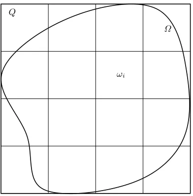
This estimate suggests looking for partitions∆that minimize diam(∆) pro-vided the number of cells N =|∆| is fixed. Clearly, diam(∆) ≥ CN−1/d for some constant C independent of N, and the order N−1/d is achieved if we for example choose a (hyper)cubeQcontaining Ω, split it uniformly intoNd equal subcubes Qi, and define the cells of ∆ by intersecting Ω with these subcubes,ωi =Ω∪Qi, see Fig. 1. This gives a simple algorithm for piecewise constant approximation with approximation orderN−1/d for all f ∈W1
Q
ωi
[image:5.595.186.382.123.322.2]Ω
Fig. 1.Uniform partition.
Algorithm 1 Define ∆ by splitting Ω = (0,1)d into N = md cubes ω1, . . . , ωN of edge length h= 1/m. Let s∆(f) be given by (2).
Theorem 1.The error of the piecewise constant approximation s∆(f) gen-erated by Algorithm 1 satisfies
kf −s∆(f)kp ≤C(d, p)N−1/d|f|W1
p(Ω), f ∈W
1
p(Ω), 1≤p≤ ∞. (4)
The order N−1/d in (4) means that an approximation with error kf − s∆(f)kp =O(ε) is only achieved using (1ε)d degrees of freedom, which grows exponentially fast with the number of dimensions d. This phenomenon is often referred to as curse of dimensionality.
The approximation orderN−1/din (4) cannot be improved in general. See [14, Section 6.2] for a discussion of saturation and inverse theorems, where certain smoothness properties off are deduced from appropriate assumptions about the order of its approximation by multivariate piecewise polynomials. For example, assuming that E(f, ∆)∞=o(diam(∆)) as diam(∆)→0 for all
partitions∆, we can easily show thatf is a constant function. Indeed, for any x, y ∈Ω we can find a partition ∆such thatx andy belong to the same cell ω, and diam(ω) = diam(∆)≤2kx−yk2. Then|f(x)−f(y)| ≤ |f(x)−fω|+
|fω −f(y)| ≤4E(f, ∆)∞ =o(diam(ω)). Hence |f(x)−f(y)|= o(kx−yk2)
A saturation theorem in terms of the number of cells holds for any se-quence of ‘isotropic’ partitions. We say that a sese-quence of partitions {∆N} isisotropic if there is a constant γ such that
diam(ω)≤γρ(ω) for all ω ∈[ N
∆N,
whereρ(ω) is the maximum diameter ofd-dimensional balls contained in ω. Note that an isotropic partition may contain cells of very different sizes, see for example Fig. 2 below.
Theorem 2.Assume that f ∈ C1(Ω) and there is an isotropic sequence of
partitions {∆N} with lim
N→∞diam(∆N) = 0 such that
E(f, ∆N)∞=o(|∆N|−1/d), N → ∞.
Thenf is a constant.
Proof. If f is not constant, then the gradient ∇f := [∂f /∂xi]d
i=1 is nonzero
at a point ˆx ∈ Ω. Since the gradient of f is continuous, there is δ > 0, a unit vector σ and a cube Q ⊂ Ω with edge length h containing ˆx such that Dσf(x) ≥δ for all x ∈Q, where Dσf =∇fTσ denotes the directional derivative of f. The cube ˜Q := {x ∈ Q : dist(x, ∂Q) > h/4} has edge lengthh/2 and volume (h/2)d. Assume thatN is large enough to ensure that diam(∆N) < h/4. Then any cell ω ∈ ∆N that has nonempty intersection with ˜Q is contained in Q. If [x1, x2] is an interval in ω parallel to σ, then
|f(x2)−f(x1)| ≥ δkx2 −x1k2, which implies |f(x2)−f(x1)| ≥ δρ(ω) and
hence
εN :=E(f, ∆N)∞≥E(f)L∞(ω) ≥
δ
2ρ(ω)≥ δ
2γ diam(ω). Therefore
vol(ω)≤µd γ
δ d
εdN,
where µd denotes the volume of the d-dimensional ball of radius 1. Since ˜Q is covered by such cellsω, we conclude that
h
2 d
= vol( ˜Q)≤ X ω∩Q˜6=∅
vol(ω)≤µd γ
δ d
εd N|∆N|,
E(f, ∆N)∞≥
hδ
2γµ1d/d|∆N|
−1/d,
contrary to the assumption. ⊓⊔
Sobolev-Poincar´e inequalities
Sobolev-Poincar´e inequalities provide bounds for the error of f −fω. They hold on domains satisfying certain geometric conditions, for example the interior cone condition or the Lipschitz boundary condition. In some cases even a necessary and sufficient condition for ω to admit such an inequality is known. A domain ω ⊂Rd is called aJohn domain if there is a fixed point
x0 ∈ω and a constant cJ >0 such that every pointx ∈ω can be connected to x0 by a curve γ ⊂ω such that
dist(y, ∂ω)≥cJℓ(γ(x, y)), for all y∈γ,
where ℓ(γ(x, y)) denotes the length of the segment of γ between x and y. Every domain with the interior cone condition is a John domain, but not otherwise. In particular, there are John domains with fractal boundary of Hausdorff dimension greater than d−1.
The following variant of Sobolev inequality holds for all John domains ω ⊂Rd, see [18] and references therein,
kf−fωkLq∗(ω) ≤C(d, q, λ)k∇fkLq(ω), f ∈W
1
q(ω), 1≤q < d, (5)
where q∗ = dq/(d −q) is the Sobolev conjugate of q, and λ is the John
constant of ω. Note that k∇fkLq(ω) denotes the Lq-norm of the euclidean
norm of ∇f, that isk∇fkqLq(ω) =R ω
Pd
i=1|∂f /∂xi|2
q/2
dx, which is equiv-alent to the more standard seminorm of the Sobolev space W1
q(ω) given by
|f|qW1
q(ω) =
Pd i=1
R
ω|∂f /∂xi|qdx. We prefer using k∇fkLq(ω) because of the
explicit expressions for C(d, q, λ) available in certain cases, see the end of this section.
According to [7], if the Sobolev inequality (5) holds for some 1≤q < dand certain mild separation condition (valid for example for any simply connected domain in R2) is satisfied, then ω is a John domain.
kf−fωkLp(ω) ≤ |ω|
1
p−
1
τ∗
kf−fωkLτ∗(ω) ≤C(d, τ, λ)|ω|1p−τ1∗
k∇fkLτ(ω)
≤C(d, τ, λ)|ω|1d+
1
p−
1
qk∇fk
Lq(ω),
and we arrive at the following Sobolev-Poincar´e inequality for all p, q such that 1≤p < ∞ and τ ≤q ≤ ∞,
kf−fωkLp(ω) ≤C(d, p, λ)|ω|
1
d+1p−1qk∇fk
Lq(ω), f ∈W
1
q(ω). (6)
In particular, sinceτ ≤p, we can chooseq =p, which leads to the Poincar´e inequality for bounded John domains for all 1≤p <∞ in the form
kf −fωkLp(ω)≤Cdiam(ω)k∇fkLp(ω), f ∈W
1
p(ω), (7)
whereC depends only on d, p, λ.
Poincar´e inequality in the case p = ∞ has been considered in [25]. If ω⊂Rd is a bounded path-connected domain, then
E(f)L∞(ω)≤r(ω)k∇fkL∞(ω), with r(ω) := inf
x∈ωsupy∈ωρω(x, y),
whereρω(x, y) is the geodesic distance, i.e. the infimum of the lengths of the paths inω from x toy.
If ω is star-shaped with respect to a point, then r(ω)≤ diam(ω), and so (7) holds with C = 2 for all such domains if p =∞. Moreover, as observed in [25], the arguments of [2, 11] can be applied to show that for any bounded star-shaped domain
kf −fωkLp(ω)≤
2
1−d/pdiam(ω)k∇fkLp(ω), f ∈W
1
p(ω), d < p≤ ∞. (8)
In particular, (8) applies to star-shaped domains with cusps that fail to be John domains.
If ω is a bounded convex domain in Rd, then (7) holds for all 1 ≤p≤ ∞
with a constantCdepending only ond[12]. Moreover, optimal constants are known for p = 1,2: C = 1/π for p = 2 [22, 3] and C = 1/2 for p = 1 [1]. Sincer(ω) = 12 diam(ω), it follows that (7) holds with C = 1 ifp=∞.
3 Nonlinear approximation
We have seen in Section 2 that the approximation order N−1/d is the best achievable on isotropic partitions. Nevertheless, by using more sophisticated algorithms the estimate (4) can be improved in the sense that the norm
|f|W1
p(Ω) in its right hand side is replaced by a weaker norm, for example
|f|W1
q(Ω) withq < p. This improvement is often quite significant bacause the
norm |f|W1
q(Ω) is finite for functions with more substantial singularities than
those allowed in the space W1
p(Ω), see [14] for a discussion.
Recall that in Algorithm 1 the partition ∆ is independent of the target function f, and so s∆(f) depends linearly on f. A simple example of a non-linear algorithm is given by Kahane’s approximation method for continuous functions of bounded total variation on an interval, see [14, Section 3.2]. To define a partition of the interval (a, b), the points a=t0 < t1 <· · ·< tN =b are chosen such that var(ti−1,ti)(f) =
1
N var(a,b)(f), i = 1, . . . , N −1. By set-ting ωi = (ti−1, ti),ci = (Mωif+mωif)/2, we see that the piecewise constant
function s = PNi=1−1ciχωi satisfies kf −sk∞ ≤
1
2N var(a,b)(f). Thus, for the partition ∆={ωi}Ni=1−1,
E(f, ∆)∞ ≤ 21N var(a,b)(f) = 21N|f|BV(a,b)≤ 21N|f|W1 1(a,b),
where the last inequality presumes that f belongs to W1
1(a, b), that is it is
absolutely continuous and its derivative is absolutely integrable.
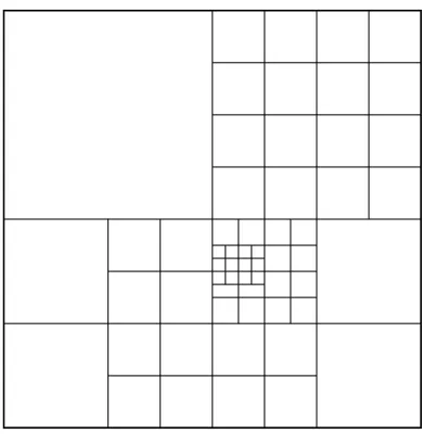
In the multivatiate case the first algorithm of this type was given in [5]. It is based on diadic partitions ∆ of Ω = (0,1)d that consist of the dyadic cubes of the form
2−jd(k1, k1+ 1)× · · · ×(kd, kd+ 1), j = 0,1,2, . . . , 0≤ki <2jd,
produced adaptively by successive diadic subdivisions of a cube into 2d equal subcubes with halved edge length, see Fig. 2.
The following lemma plays a crucial role in [5].
Lemma 1.Let Φ(ω) be a nonnegative function of sets ω ⊂Ω which is sub-additive in the sense that Φ(ω′) +Φ(ω′′) ≤ Φ(ω′∪ω′′) as soon as ω′, ω′′ are
disjoint subdomains of Ω. Given α >0, we set
gα(ω) :=|ω|αΦ(ω), ω⊂Ω,
Fig. 2.Example of a diadic partition.
Gα(∆) := max
ω∈∆gα(ω).
Assume that a sequence of partitions{∆k}∞k=0 of Ω= (0,1)dinto diadic cubes
is obtained recursively as follows. Set ∆0 = {Ω}. Obtain ∆k+1 from ∆k by the diadic subdivision of those cubes ω ∈∆k for which
gα(ω)≥2−dαGα(∆k).
Then
Gα(∆k)≤C(d, α)|∆k|−(α+1)Φ(Ω), k = 0,1, . . . .
This lemma can be used with Φ(ω) = |f|qW1
q(ω), 1 ≤ q < ∞, which is
obviously subadditive, giving rise to the following algorithm which we only formulate for piecewise constants even though the results in [5] also apply to the higher order piecewise polynomials.
Algorithm 2 ([5]) Suppose we are interested in the approximation in Lp norm, 1 < p ≤ ∞. Choose 1 ≤ q < ∞ such that q > τ := 1+dd/p (τ = d if p = ∞), and assume that f ∈ W1
q(Ω), Ω = (0,1)d. Set ∆0 = {Ω}. While
|∆k| < N, obtain ∆k+1 from ∆k by the diadic subdivision of those cubes ω∈∆k for which
gα(ω)≥2−dαmax
where
gα(ω) :=|ω|α|f|qW1
q(ω), α=
q τ −1.
Since |∆k|<|∆k+1|, the subdivisions terminate at some∆=∆m with |∆| ≥ N and |∆| = O(N). The resulting piecewise constant approximation s∆(f) of f is given by (2).
Theorem 3 ([5]). The error of the piecewise constant approximations∆(f) generated by Algorithm 2 satisfies
kf −s∆(f)kp ≤C(d, p, q)N−1/d|f|W1
q(Ω), f ∈W
1
q(Ω). (9)
Proof. We only consider the case p < ∞. For any ω ∈ ∆ it follows by the Sobolev-Poincar´e inequality (6) for cubes that
kf−fωkpLp(ω) ≤C1|ω|
p d+1−
p q|f|p
W1
q(ω) =C1g
p/q
α (ω)≤C1Gp/qα (∆), where C1 depends only ond, p, q. Hence
kf−s∆(f)kpp = X
ω∈∆
kf −fωkpLp(ω) ≤C1|∆|G
p/q α (∆).
Now Lemma 1 implies
kf −s∆(f)kp ≤C2|∆|1/p|∆|−(α+1)/qΦ1/q(Ω) =C2|∆|−1/d|f|W1
q(Ω). ⊓⊔
If q ≥ p, then the estimate (9) is also valid for the much simpler Algo-rithm 1. Therefore the scope of AlgoAlgo-rithm 2 is when f ∈ W1
q(Ω) for some q satisfying τ < q < p but f /∈ W1
p(Ω) or if |f|W1
q(Ω) is significantly smaller
than |f|W1
p(Ω). Note that the computation of gα(ω) in Algorithm 2 requires
first order partial derivatives of f. Algorithms 2 is nonlinear (in contrast to Algorithm 1) because the partition ∆depends on the target function f.
An adaptive algorithm based on the local approximation errors rather than local Sobolev norm of f was studied in [17]. We again restrict to the piecewise constant case.
Algorithm 3 Assume f ∈ Lp(Ω), Ω = (0,1)d, for some 0 < p ≤ ∞ and choose ε > 0. Set ∆0 ={Ω}. For k = 0,1, . . ., obtain ∆k+1 from ∆k by the diadic subdivision of those cubes ω∈∆k for which
kf −fωkLp(ω) > ε.
Since kf −fωkLp(ω) → 0 as |ω| → 0, the subdivisions terminate at some
Now in contrast to [5], 0 < p < 1 is also allowed. The error bounds are obtained for functions in Besov spaces rather than Sobolev spaces. Recall that f belongs to the Besov space Bα
q,σ(Ω), α >0, 0< q, σ≤ ∞, if
|f|Bα q,σ(Ω)=
R∞
0 (t
−αω
r(f, t)q)σ dtt 1/σ
if 0< σ <∞,
supt>0t−αωr(f, t)q if σ=∞.
is finite, wherer= [α]+ 1 is the smallest integer greater thanα, andωr(f, t)q denotes ther-th modulus of smoothness off inLq. In particular,Bαq,∞(Ω) =
Lip(α, Lq(Ω)) for 0< α <1.
Theorem 4 ([17]). Let 0 < α < 1, q > α+dd/p and 0 < σ ≤ ∞. If f ∈ Bα
q,σ(Ω), then for any N there is an ε >0 such that the partition∆produced by Algorithm 3 satisfies |∆| ≤N and
kf −s∆(f)kp ≤C(d, p, q)N−α/d|f|Bα q,σ(Ω).
The set of all diadic cubes is a tree Tdc, where the children of a cube ω are the cubes ω1, . . . , ω2d obtained by its diadic subdivision. The only root
ofTdc isΩ= (0.1)d. Clearly, Algorithms 2 and 3 produce acomplete subtree
T of Tdc in the sense that for any node in T its parent and all siblings are also in T. The corresponding partition ∆ consists of all leaves of T. If we set e(ω) = kf −fωkpLp(ω), then E(T) := Pω∈∆e(ω) = kf −s∆(f)kpp. It is easy to see that|∆|= 1 + (2d−1)n(T), where n(T) denotes the number of subdivisions used to create T. The quantity n(T) measures the complexity of a tree, and En := infn(T)≤nE(T) gives the optimal error achievable by a tree of a given complexity. It is natural to look for optimal or near optimal trees. The concept oftree approximation was introduced in [8] in the context of n-term wavelet approximation. General results applicable in particular to the piecewise constant approximations on diadic partitions are given in [4]. The idea is that replacing kf −fωkLp(ω) > ε in Algorithm 3 by a more
sophisticated refinement criterion leads to an algorithm that produces a near optimal tree.
e(ω) :=kf −fωkLpp(ω)> ε+α(ω),
and define α(ωi) for all children ω1, . . . , ω2d of ω by
α(ωi) = e(ωi) σ(ω) h
α(ω) + (ε−e(ω)−σ(ω))+
i
, σ(ω) := X j
e(ωj),
assuming thatσ(ω)6= 0. The algorithm terminates at some treeT =Tm since
kf−fωkLp(ω)→0as|ω| →0. The resulting piecewise constant approximation
s∆(f)off is given by (2), where∆is the diadic partition defined by the leaves of T.
Theorem 5 ([4]). The tree T produced by Algorithm 4 is near optimal as it satisfies
E(T)≤2(2d+ 1)E[n/2], n =n(T).
Further results on tree approximation are reviewed in [15].
The above algorithms generate piecewise constant approximations by con-structing an appropriate partition of Ω. A different approach is to look for an approximation as linear combination of a fixed set of piecewise constant ‘basis functions’, for example characteristic functions of certain subsets of Ω. More general, let D ⊂ Lp(Ω) be a set of functions, called dictionary, such that the finite linear combinations of the elements in D are dense in Lp(Ω). Note that the setD does not have to be linearly independent. Given f ∈Lp(Ω), the error of the best n-term approximation is defined by
σn(f,D)p = inf s∈Σnk
f −skp,
whereΣn=Σn(D) is the set of all linear combinations of at mostnelements of D,
Σn(D) :=n X g∈D
cgg :D⊂ D, |D| ≤n, cg ∈R o
.
If the functions in D are piecewise constants, then the approximants in Σn(D) are piecewise constants as well. If each elementg ∈ Dcan be described using a bounded number of parameters, thens=P
g∈Dcgg ∈Σn(D) requires
Piecewise constant approximation s∆(f) produced by Algorithm 2 or 3 belongs to Σn(Dc), with n = |∆|, where the dictionary Dc consists of the characteristic functions χω of all diadic cubes ω ⊆ (0,1)d. Therefore Theo-rems 3 and 4 imply that
σn(f,Dc)p ≤ (
C(d, p, q)n−α/d|f| Wα
q(Ω) if f ∈W
α
q (Ω), α= 1, C(d, p, q)n−α/d|f|
Bα
q,σ(Ω) if f ∈B
α
q,σ(Ω), 0< α <1.
as soon asq > α+dd/p.
Clearly, Σn(Dc) includes many piecewise constants with more then n di-adic cells, for example,χ(0,1)2−χ(0,1/2m)2 ∈Σ2(Dc) is piecewise constant with
respect to a partition of (0,1)2 into 3m+1 diadic squares. A larger dictionary
Dr consisting of the characteristic functions of all ‘diadic rings’ (differences between pairs of embedded diadic cubes) has been considered in [9, 20]. An adaptive algorithm proposed in [9] produces a piecewise constant approxi-mations∆(f) of any functionf of bounded variation, where ∆is a partition of (0,1)2 intoN diadic rings, such that
kf−s∆(f)k2 ≤18
√
3N−1/2|f|BV((0,1)2),
where |f|BV(Ω) is the variation of f over Ω. Recall that the space BV(Ω)
coincides with Lip(1, L1(Ω)) and contains the Besov space B11,1(Ω). In [20]
this result is generalized to certain spaces of bounded variation with respect to diadic rings, and to the Besov spaces, leading in particular to the estimate
σn(f,Dr)p ≤C(d, p)n−α/d|f|Bα
τ,τ(Ω), f ∈B
α
τ,τ(Ω), 0< α <1,
whereτ = α+dd/p. Recall for comparison thatq > τ in Theorems 3 and 4. An important ‘piecewise constant’ dictionary Dh is given by the multi-variate Haar wavelets. Let ψ0 = χ
(0,1) and ψ1 = χ(0,1/2) −χ(1/2,1). For any
e= (e1, . . . , ed) ∈Vd, where Vd is the set consisting of the nonzero vertices of the cube (0,1)d, let
ψe(x1, . . . , xd) := ψe1(x1)· · ·ψed(xd).
Then the set
of Haar wavelets ψe
j,k is an orthonormal basis for L2(Rd). Therefore every
f ∈L2(Rd) has anL2-convergent Haar wavelet expansion
f =X
j,k,e
hf, ψj,ke iψej,k, hf, ψj,ke i:= Z
Rd
f(x)ψej,k(x)dx.
If f ∈ L2(Ω), Ω = (0,1)d, then f −fΩ has zero mean on (0,1)d and hence by extending it to Rd by zero and taking a Haar wavelet decomposition, we
obtain an L2-convergent series
f =fΩ+ X
(j,k,e)∈ΛΩ
fj,k,eψj,ke , (10)
where ΛΩ denotes the set of indices (j, k, e) such that suppψej,k ⊆ Ω, and fj,k,e are theHaar wavelet coefficients of f,
fj,k,e = Z
(0,1)d
f(x)ψj,ke (x)dx.
Clearly, the Haar wavelet coefficients are well defined for any function f ∈ L1(Ω). The series (10) converges unconditionally in Lp-norm if f ∈ Lp(Ω), 1 < p < ∞. This implies in particular that every subset of {kfj,k,eψej,kkp : (j, k, e) ∈ ΛΩ} has a largest element. The dictionary of Haar wavelets on Ω = (0,1)d is given by
Dh ={ψej,k : (j, k, e)∈ΛΩ}.
A standard approximation method for this dictionary is thresholding, also called greedy approximation.
Algorithm 5 (Haar wavelet thresholding) Assume f ∈ Lp(Ω), Ω = (0,1)d, for some 1 < p < ∞. Let R
Ωf(x)dx = 0. (Otherwise, replace f by f − fΩ.) Given n ∈ N, choose n largest elements in the sequence
{kfj,k,eψj,ke kp : (j, k, e) ∈ ΛΩ} and denote the set of their indices by ΛnΩ. The resulting approximation of f is given by
Gn(f) = X
(j,k,e)∈Λn Ω
fj,k,eψej,k.
Theorem 6 ([9]). Let f ∈ BV(Ω), Ω = (0,1)2, and R
Ωf(x)dx = 0. Then the approximationGn(f) produced by Algorithm 5 satisfies
kf −Gn(f)k2 ≤C n−1/2|f|BV(Ω),
where C = 36(480√5 + 168√3).
It turns out thatGn(f) is also near best for any 1< p <∞.
Theorem 7 ([24]). Let f ∈ Lp(Ω), Ω = (0,1)d, for some 1 < p < ∞, and R
Ωf(x)dx= 0. The approximation Gn(f) produced by Algorithm 5 satisfies
kf−Gn(f)kp ≤C(d, p)σn(f,Dh)p.
An estimate for σn(f,Dh)p follows from the results of [16] by using the extension theorems for functions in Besov spaces, see [14, Section 7.7].
Theorem 8 ([16]).Let1< p <∞, 0< α <1/p,τ = α+dd/p. Iff ∈Bα τ,τ(Ω), Ω= (0,1)d, and R
Ωf(x)dx= 0, then
σn(f,Dh)p ≤C(d, p)n−α/d|f|Bα τ,τ(Ω).
The best n-term approximation by piecewise constants (and by piecewise polynomials of any degree) on hierarchical partitions of Rd or (0,1)d into
anisotropic diadic boxes of the form
k1 2j1d,
k1+ 1
2j1d
× · · · ×2kjddd,kd+ 1 2jdd
, js, ks∈Z,
has been studied in [23]. Here, the smoothness of the target function is expressed in terms of certain Besov-type spaces defined with respect to a given hierarchical partition. In [21], results of the same type are obtained for even more flexible anisotropic hierarchical triangulations. LetT =∪m∈Z∆m, where each ∆m is a locally finite triangulation of R2 such that ∆m+1 is
ob-tained from ∆m by splitting each triangle ω ∈ ∆m into at least two and at most M subtriangles (children). The hierarchical triangulation T is called weak locally regular if there are constants 0 < r < ρ < 1 (r ≤ 1
4), such
that for any ω ∈ T it holds r|ω′| ≤ |ω| ≤ ρ|ω′|, where ω′ ∈ T is the parent
triangle of ω. Clearly, the triangles in T may have arbitrarily small angles. The skinny B-space Bα,k
q (T), 0 < q < ∞, α > 0, k ∈ N, is the set of all f ∈Lloc
|f|Bα,k q (T) :=
X
ω∈T
|ω|−αqwk(f, ω)qq1/q,
where
wk(f, ω)q := sup h∈R2k
δhk(f)kLq(ω),
δhk(f) being the k-th finite difference of f, in particular
δ1
h(f, x) := (
f(x+h)−f(x), if [x, x+h]⊂ω,
0, otherwise.
It is shown in [21] that if T is regular, i.e. there is a positive lower bound for the minimum angles of all triangles in T, then Bα,k
q (T) =Bq,q2α(R2) with equivalent norms whenever 0<2α <min{1/q, k}.
Consider the dictionary DT ={χ
ω :ω ∈ T }.
Theorem 9 ([21]). Let 0 < p < ∞, α > 0, τ = α+22/p. If f ∈ B
α
2,1
τ (T)∩ Lp(R2), then
σn(f,DT)p ≤C(p, α, ρ, r)n−α/2|f| B
α
2,1
τ (T).
Note that certain Haar type bases can be introduced on the anisotropic diadic partitions and on hierarchical triangulations obtained by a special refinement rule, see [23, 21] for their definition and approximation properties. An extension of Theorem 9 to Rd with d >2 is given in [13].
4 Anisotropic partitions
We have seen in Theorem 2 that piecewise constants on isotropic parti-tions cannot approximate nontrivial smooth funcparti-tions with order better than N−1/d. We now turn to the question what approximation order can be achieved on anisotropic partitions. An argument similar to that in the proof of Theorem 2 shows that it is not better than N−2/(d+1) if we assume
that the partition is convex, i.e. all its cells are convex sets.
Theorem 10 ([10]).Assume thatf ∈C2(Ω)and the Hessian off is positive
definite at a point xˆ ∈ Ω. Then there is a constant C depending only on f and d such that for any convex partition ∆ of Ω,
The order of piecewise constant approximation on anisotropic partitions in two dimensions has been investigated in [19]. It is shown that for any f ∈ C2([0,1]2) there is a sequence of partitions ∆
N of (0,1)2 into polygons with the cell boundaries consisting of totally O(N) straight line segments, such that kf −s∆N(f)k∞ = O(N
−2/3). Moreover, the approximation order
N−2/3cannot be improved on such partitions. Note that by triangulating each
polygonal cell of ∆N one obtains a convex partition with O(N) triangular cells, so that Theorem 10 also applies, giving the same saturation orderN−2/3.
Another result of [19] is that for any f ∈ C3([0,1]2) there is a sequence
of partitions ∆N of (0,1)2 into cells with piecewise parabolic boundaries defined by a total ofO(N) parabolic segments (pieces of graphs of univariate quadratic polynomials) such thatkf −s∆N(f)k∞=O(N
−3/4).
The following algorithm achieves the approximation order N−2/(d+1) on
convex polyhedral partitions with totallyO(N) facets.
Algorithm 6 ([10]) Assume f ∈ W1
1(Ω), Ω = (0,1)d. Split Ω into N1 =
mdcubesω
1, . . . , ωN1 of edge lengthh= 1/m. Then split eachωi intoN2 slices
ωij, j = 1, . . . , N2, by equidistant hyperplanes orthogonal to the average
gra-dient gi :=|ωi|−1 R
ωi∇f on ωi. Set ∆={ωij :i= 1, . . . , N1, j = 1, . . . , N2},
and define the piecewise constant approximations∆(f)by (2). Clearly,|∆|= N1N2 and each ωij is a convex polyhedron with at most 2(d+ 1) facets.
This algorithm is illustrated in Fig. 3.
Theorem 11 ([10]). Assume that f ∈ W2
p(Ω), Ω = (0,1)d, for some 1 ≤ p≤ ∞. For anym = 1,2, . . ., generate the partition∆m by using Algorithm 6 with N1 =md and N2 =m. Then
kf−s∆m(f)kp ≤C(d, p)N
−2/(d+1)(
|f|W1
p(Ω)+|f|Wp2(Ω)), (11)
where N =|∆m|=md+1.
Proof. For simplicity we assume d = 2 and p = ∞. (The general case is treated in [10].) Let us estimate the error of the best approximation of f by constants on ωij,
E(f)L∞(ωij)=
1 2
max x∈ωij
f(x)− min x∈ωij
f(x).
Let σi be a unit vector orthogonal to gi. Since ∇f is continuous, there is ˜
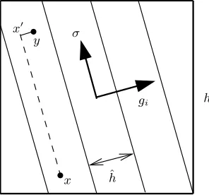
Fig. 3.Algorithm 6 (d= 2,m= 4). The arrows stand for the average gradientsgi on the cubes
ωi. The cellsωij are shown only for one cube.
c1h|f|W∞2(ωi). Given x, y ∈ ωij, choose a point x′ ∈ ωij such thaty−x′ and
x′−xare collinear withgi andσi, respectively. (This is always possible if we swap the roles of x and y when necessary, see Fig. 4.)
h
ˆ
h gi
σ
x y x′
Fig. 4. Illustration of the proof of Theorem 11, showing a singleωi.
[image:19.595.207.355.437.575.2]|f(y)−f(x)| ≤ |f(y)−f(x′)|+|f(x′)−f(x)|
≤ˆhk∇fkL∞(ωij)+c2hkDσfkL∞(ωij)
≤c3(ˆh|f|W∞1(ωij)+h2|f|W∞2(ωi))
≤c4m−2(|f|W∞1(ωij)+|f|W∞2(ωi)).
Thus,
kf −fωijkL∞(ωij) ≤2E(f)L∞(ωij)≤c4m
−2(
|f|W∞1(Ω)+|f|W∞2(Ω)),
and (11) follows. ⊓⊔
The improvement of the approximation order by piecewise constants from N−1/d on isotropic partitions to N−2/(d+1) on convex partitions does not
extend to higher degree piecewise polynomials. Given a partition ∆, let E1(f, ∆)p denote the best error of (discontinuous) piecewise linear
approxi-mation in Lp-norm. Then the approximation order on isotropic partitions is N−2/dfor sufficiently smooth functions, and it cannot be improved in general on any convex partitions.
Theorem 12 ([10]).Assume thatf ∈C2(Ω)and the Hessian off is positive
definite at a point xˆ ∈ Ω. Then there is a constant C depending only on f and d such that for any convex partition ∆ of Ω,
E1(f, ∆)∞≥C|∆|−2/d.
References
1. G. Acosta and R. G. Dur´an: An optimal Poincar´e inequality inL1 for convex domains, Proc. Amer. Math. Soc.132, 2004, 195–202.
2. R. Arcangeli and J. L. Gout: Sur l’evaluation de l’erreur d’interpolation de Lagrange dans un ouvert deRn, R.A.I.R.O. Analyse Numerique10, 1976, 5–27.
3. M. Bebendorf: A note on the Poincar´e inequality for convex domains, J. Anal. Appl. 22, 2003, 751–756.
4. P. Binev and R. DeVore: Fast computation in adaptive tree approximation, Numer. Math.
97, 2004, 193–217.
5. M. S. Birman and M. Z. Solomyak: Piecewise polynomial approximation of functions of the classes Wα
p, Mat. Sb. 73 (115), no. 3, 1967, 331–355 (in Russian). English translation in
Math. USSR-Sb.2, no. 3, 1967, 295-317.
6. S. Brenner and L. R. Scott:The Mathematical Theory of Finite Element Methods. Springer-Verlag, Berlin, 1994.
8. A. Cohen, W. Dahmen, I. Daubechies, and R. DeVore: Tree approximation and optimal encoding, Appl. Comp. Harm. Anal.11, 2001, 192–226.
9. A. Cohen, R. DeVore, P. Petrushev, and H. Xu: Nonlinear approximation and the space
BV(R2), Amer. J. Math.121, 1999, 587–628.
10. O. Davydov, Approximation by piecewise constants on convex partitions, in preparation. 11. L.T. Dechevski and E. Quak: On the Bramble-Hilbert lemma, Numer. Funct. Anal. Optim.11,
1990, 485–495.
12. S. Dekel and D. Leviatan: The Bramble-Hilbert lemma for convex domains, SIAM J. Math. Anal.35, 2004, 1203–1212.
13. S. Dekel and D. Leviatan: Whitney estimates for convex domains with applications to mul-tivariate piecewise polynomial approximation, Found. Comput. Math.4, 2004, 345–368. 14. R. A. DeVore: Nonlinear approximation, Acta Numerica7, 1998, 51–150.
15. R. A. DeVore: Nonlinear approximation and its applications, in R. DeVore and A. Kunoth (eds.): Multiscale, Nonlinear and Adaptive Approximation - Dedicated to Wolfgang Dahmen on the Occasion of his 60th Birthday. Springer-Verlag, Berlin, 2009, 169–201.
16. R. DeVore, B. Jawerth and V. Popov: Compression of wavelet decompositions, Amer. J. Math.
114, 1992, 737–785.
17. R. A. DeVore and X. M. Yu: Degree of adaptive approximation, Math. Comp. 55, 1990, 625–635.
18. P. Haj lasz: Sobolev inequalities, truncation method, and John domains, inPapers on Anal-ysis: A volume dedicated to Olli Martio on the occasion of his 60th birthday. Report. Univ. Jyv¨askyl¨a83, 2001, 109–126.
19. A. S. Kochurov: Approximation by piecewise constant functions on the square, East J. Ap-prox.1, 1995, 463–478.
20. Y. Hu, K. Kopotun and X. Yu: On multivariate adaptive approximation, Constr. Approx.
16, 2000, 449–474.
21. B. Karaivanov, P. Petrushev, Nonlinear piecewise polynomial approximation beyond Besov spaces, Appl. Comput. Harmon. Anal. 15 (2003), No. 3, 177-22
22. L. E. Payne and H. F. Weinberger: An optimal Poincar´e inequality for convex domains, Arch. Rational Mech. Anal.5, 1960, 286–292.
23. P. Petrushev: Multivariate n-term rational and piecewise polynomial approximation, J. Ap-prox. Theory121, 2003, 158–197.
24. V. Temlyakov: The bestm-term approximation and greedy algorithms, Adv. Comput. Math.
8, 1998, 249–265.