Evidence-Based Robust Design of Deflection Actions
for Near Earth Objects
Federico Zuiani PhD Candidate,
School of Engineering, University of Glasgow, James Watt South Building, Glasgow, G12 8QQ, United Kingdom Tel.: +44-141-5484558
Massimiliano Vasile Reader,
Department of Mechanical & Aerospace Engineering, University of Strathclyde, 75 Montrose Street, Glasgow, G1 1XJ, United Kingdom
Tel.: +44-141-3306465 Fax: +44-141-3305560
Alison Gibbings PhD Candidate,
School of Engineering, University of Glasgow, James Watt South Building, Glasgow, G12 8QQ, United Kingdom Tel.: +44-141-5484558
Abstract. This paper presents a novel approach to the robust design of deflection actions for Near Earth Objects
(NEO). In particular, the case of deflection by means of Solar-pumped Laser ablation is studied here in detail. The basic idea behind Laser ablation is that of inducing a sublimation of the NEO surface, which produces a low thrust thereby slowly deviating the asteroid from its initial Earth threatening trajectory. This work investigates the integrated design of the Space-based Laser system and the deflection action generated by laser ablation under uncertainty. The integrated design is formulated as a multi-objective optimisation problem in which the deviation is maximised and the total system mass is minimised. Both the model for the estimation of the thrust produced by surface laser ablation and the spacecraft system model are assumed to be affected by epistemic uncertainties (partial or complete lack of knowledge). Evidence Theory is used to quantify these uncertainties and introduce them in the optimisation process. The propagation of the trajectory of the NEO under the laser-ablation action is performed with a novel approach based on an approximated analytical solution of Gauss’ Variational Equations. An example of design of the deflection of asteroid Apophis with a swarm of spacecraft is presented.
KEYWORDS: Robust design optimisation, Evidence theory, Analytical low-thrust formulas, Perturbative expansions, Asteroid deflection
1. Introduction
During the last two decades, Near Earth Objects (NEO) have attracted considerable interest from the scientific community in general and in particular in the space field. The reasons for this are twofold: first, from a strictly scientific point of view, asteroids can provide precious data to reconstruct the genesis of the solar system. In this sense, NEOs, in contrast to other small celestial bodies, are relatively easy to reach and explore, thanks to their small dimensions, lack of atmosphere and vicinity to the Earth. On the exploration side, there is a number of past or ongoing missions aimed at the study of small celestial bodies, such as NEAR (McAdams et al. 2000), Rosetta (Glassmeier et al., 2007), Deep Space 1 (Rayman et al. 2000), Hayabusa (Nakamura and Michel 2009), Deep Impact (Hampton et al. 2005) and Dawn (Russel et al. 2007).
The second reason instead is linked with the potential threat they represent for our planet. According to the most recent tracking data, over 1000 NEOs have been classified as potentially hazardous to the Earth, i.e. they have an Earth Minimum Orbit Intersection Distance (MOID) of 0.05 AU or less and an absolute magnitude of 22.0 or less (JPL 2012). This suggests that the danger of a catastrophic event in the mid to long term is not unrealistic. The historical perspective of past impact events (e.g. Tunguska in 1908) is an important reminder of the dire consequences this could have on our fragile ecosystem.
Therefore, the scientific community has proposed a number of mitigation strategies and techniques to counteract the hazard of a NEO impact. The first serious technical study, Project Icarus (MIT 1968), dates back to 1967 but only in the 90s the theme has started to be widely explored by scientists and engineers and various strategies have been proposed. Among them we find techniques producing an impulsive change in the asteroid motion such as Nuclear blast (Smith, Barrera et al. 2004) and Kinetic Impactor (McInnes 2004), or attached Chemical engines (Scheeres and Schweickart 2004); there are others which produce a continuous low thrust like in the case of using attached Electrical thrusters (Scheeres and Schweickart 2004), or electrically propelled gravitational tugs (Lu and Love 2005), or by means of the low thrust produced by surface Ablation, the latter induced either by solar collectors (Melosh and Nemchinov 1994) or laser beam (Campbell, Phipps et al. 2003). Other more exotic systems include Mass Drivers (Olds, Charania and Schaffer 2007), which involve the controlled ejection of asteroid’s surface material in order to produce a series of small impulsive changes in its motion; there are proposals also for passive methods, like the idea of painting part of the asteroid to modify its optical properties and thus take advantage of the Yarkovsky effect (Spitale 2002).
A recent study (Sanchez, Colombo et al. 2009) presented a quantitative comparison of different deflection methodologies that suggested that surface ablation techniques could represent an advantage compared to other methodologies.
sensitivity to identify which epistemic uncertainty is the most significant in the context of asteroid deflection with laser ablation.
2. Trajectory and Deflection Model
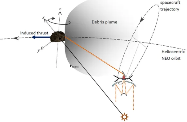
In order to assess the performance of the laser ablation approach, a hypothetical asteroid based on 99942 Apophis is considered. Its orbital elements are suitably modified in order for it to intercept the Earth in 2036. The effectiveness of the deflection action is measured by the magnitude of the impact parameter b with respect to the Earth at the time of the expected collision, as shown in Fig. 1 where
V
∞is the incoming velocity of the asteroid andE
[image:3.595.119.527.501.671.2]v
is the velocity of the Earth. The impact parameter is computed by projecting the deviated position of the asteroid on the Earth’s b-plane at the epoch of the expected impact (Vasile and Colombo 2008). In this case study, the undeviated orbit has b=0.Fig. 1 Impact parameter
The computation of b requires the variation of the orbital elements due to the deflection action. From the variation of the orbital elements one can use the deflection formulas in (Colombo et al. 2009) or the nonlinear proximal motion equations in (Vasile and Maddock 2010) to compute the position and velocity relative to the Earth. The variation of the orbital elements is obtained by integrating Gauss’ Variational Equations in non-singular equinoctial elements, (Battin 1999):
(
)
2
2 1
1
1 2
2
1 2
1
1 1 2
sin cos cos cos cos sin
cos cos cos 1 sin cos sin ( cos sin ) sin
cos cos cos 1 sin cos sin (
da a p
P L P L
dt h r
dP r p p
L P L P Q L Q L
dt h r r
dP r p p
L P L P Q
dt h r r
ε β α ε β α
ε β α ε β α ε β
ε β α ε β α
= − +
= − ⋅ + + + − −
= − ⋅ + + + −
(
)
(
)
(
)
2
2 2
1
1 2
2 2
2
1 2
1 2
3
cos sin ) sin
1 sin sin
2
1 cos sin
2
cos sin sin
L Q L dQ r
Q Q L
dt h dQ r
Q Q L
dt h
dL r
Q L Q L
dt a h
ε β
ε β
ε β
µ ε β
−
= + + ⋅
= + + ⋅
= − −
(1)
(
)
(
)
1 2
1
2
sin
cos
tan
sin
2
tan
cos
2
a
P
e
P
e
i
Q
i
Q
L
ω
ω
ω θ
=
Ω +
=
Ω +
=
Ω
=
Ω
= Ω + +
(2)
and a is the semi-major axis, e the eccentricity, i the inclination, Ω the right ascension of the ascending node
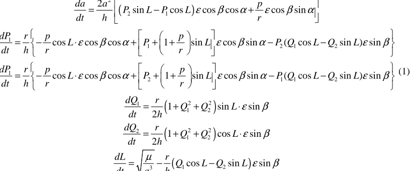
(RAAN), ω the argument of periapsis, θ the true anomaly, r is the radius, h the angular momentum, p the semi-latus rectum, µ the gravity constant of the central body and L the true longitude. ε, α and β are respectively the modulus, azimuth and elevation of the thrust acceleration in the radial-transversal reference frame, as in Fig. 2, forming the thrust vector:
[
cos
cos
sin
cos
sin
]
Tε
α
β
α
β
β
=
f
(3) [image:4.595.220.378.393.588.2]Numerical integration of Gauss’ Variational equations would be too computationally expensive for the analyses in this paper, as thousands of trajectories need to be evaluated. Hence, Gauss’ equations are here integrated using Finite Perturbative Elements in Time (FPET). FPET are based on an approximated analytical solution of Gauss’ equations over short arcs for a constant thrust (Palmas 2010; Zuiani, Vasile et al. 2011). The next section will describe the derivation of the FPET approach.
Fig. 2 Radial-transversal reference frame
2.1 The Low Thrust Perturbative Approach
( )
( )
(
)
( )
( )
(
)
( )
( )
(
)
( )
( )
(
)
( )
( )
(
)
( )
(
)
(
)
0 0 1
1 10 0 11
2 20 0 21
1 10 0 11
2 20 0 21
00 0 11
, ,
, ,
, ,
, ,
, ,
,
, ,
a L
a
L
a
L
P L
P
L
P
L
P L
P
L
P
L
Q L
Q
L
Q
L
Q
L
Q
L
Q
L
t L
t
L
L
t
L
ε
α β
ε
α β
ε
α β
ε
α β
ε
α β
ε
α β
=
+
∆
=
+
∆
=
+
∆
=
+
∆
=
+
∆
=
∆ +
∆
(4)
where:
0
L
=
L
+ ∆
L
(5)The zero-order terms, obtained for ε = 0 correspond to the unperturbed Keplerian motion. Once the analytical expressions for a1(L), P11(L), P21(L), Q11(L), and Q21(L) are available, together with t00(L) and t11(L), the variations of the five orbital parameters and time are known as a first order approximated function of the true longitude L, with respect to the reference state at L0. Thus, one can analytically propagate the non-singular elements, either backward
or forward in L, for an arbitrary set of initial (final) conditions and control force components, expressed in terms of magnitude and two angles (Palmas 2010).
Motion propagation is obtained by subdividing the trajectory into Finite Perturbative Elements in Time, i.e. a number of arcs each characterised by a constant thrust acceleration vector in the radial transversal reference frame (as shown in Fig. 3). Within each arc, forward propagation of the motion is performed analytically.
Fig. 3 Low Thrust trajectory subdivided in FPET arcs
In a previous work (Zuiani, Vasile et al. 2011) it was shown that this analytical propagation with FPET allows for computational times of at least one order of magnitude lower than numerical integration but with comparable accuracy. In this paper, at the beginning of each trajectory arc, the thrust acceleration acting on the NEO is computed by evaluating the ablation model (see Section 4.). Since, in general, the thrust magnitude varies with a periodic pattern along the trajectory, the ablation model needs to be evaluated quite often. The frequency with which the model is evaluated dictates the amplitude of the trajectory arcs. The basic idea is to have short arcs when the thrust is high and larger ones when the thrust is low. In order to achieve this, during the propagation the arc length ∆L is dynamically adjusted with the simple law:
10 10
log
log
1
min
exp
maxmax
L
A
L
k
ε
ε
−
+
+
∆ =
∆
(6)where
ε
is the current value of the thrust acceleration,ε
max is the largest value it has assumed so far and A, k and maxL
∆
are constants which were tuned empirically in order to achieve a good compromise between accuracy and CPU cost compared to the numerical integration. This was done by performing a high number of propagations of the trajectory and ablation models with different candidate sets of tuning parameters. As a result, the set which guaranteed a negligible error on the impact parameter b with respect to the numerical integration at the lowestcomputational cost was chosen. As an example, using FPET to propagate the trajectory and ablation models implemented in Matlab® on a Intel Core Duo® 3.16 GHz machine running Windows 7® e requires between 0.2 and 2 seconds (depending on the length of the trajectory), compared with up to 30 seconds when using numerical propagation.
3. Spacecraft System Model
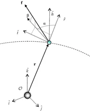
The solar-pumped laser ablation concept envisions the use of a formation of nsc identical spacecraft, each
[image:6.595.151.455.247.445.2]provided with a solar-pumped laser system. These will be flying in the proximity of the asteroid (see Fig. 4) with a distance from the asteroid’s surface between 1 and 4 km (Vasile and Maddock 2008). Note that the plume shape in Fig. 4 is a qualitative depiction of the contamination model by Kahle et al. (2006) as in Section 4.
Fig. 4 Spacecraft’s proximal motion with respect to the asteroid
Each spacecraft in the formation (see Fig. 5) is composed of a large primary mirror M1, which focuses the solar rays on a smaller secondary mirror M2. The solar rays are then conveyed onto a solar array S, which powers a laser plus other subsystems. The laser beam is directed towards the NEO by means of a directional mirror Md. A set of radiators dissipates the excess heat in order to keep the temperature of the solar array and the laser within operational limits.
Fig. 5 Laser spacecraft system
The dry mass of the spacecraft is computed as:
(
)
dry dry C S M L R bus
where mC is the mass of the harness, mS is the mass of the solar arrays, mM is the mass of the mirrors, mL is the laser
mass, mR is the radiator mass and mbus is the mass of the bus and the constant kdry represents the margin on dry mass.
The masses of the various subsystems are computed with simple analytical formulas. The harness mass is expressed as a fraction of the combined mass of the laser and solar array:
(
)
C C S L
m
=
MF
m
+
m
(8)The radiator mass AR is proportional to the area needed to dissipate the excess power. MFC is the mass fraction
for harness. The latter is computed from a steady state thermal balance between the Solar input power and the emitted power which is not reported here for the sake of conciseness.
R R R
m
=
ρ
A
(9)where ρR is the radiator specific mass per surface unit area. The mass of the solar arrays is proportional to their area
AS:
S S S S
m
=
k
ρ
A
(10)where ρS is the solar array specific mass per surface unit area and the constant kS represents the margin on solar array
mass.
The same applies to the mirror’s mass:
(
12
2)
M M M d M M
m
=
k
ρ
A
+
A
+
A
(11)where ρM is the mirror specific mass per unit area, kM is the margin on mirror mass, AM1 is the area of the primary
mirror and AM2 and Ad are the areas of the secondary and directional mirror respectively. They are defined as:
2 1
1
0.01
M M
M d
r
A
A
A
A
C
=
=
(12)where Cr is the concentration ratio, i.e. the ratio between the solar power density on the solar concentrator and that of
the spot area on the asteroid. The mass of the laser is proportional to its output power: L L L L L
m
=
k
ρ η
P
(13)where ρL is the laser specific mass per input unit power, kL is the margin on laser mass and the input power PL
depends on the solar input Pin and the efficiency of the solar array
η
SA: 1 L SA in MP
=
η
P A
(14)Finally the total mass of the spacecraft is computed by adding a fixed mass fraction for the propellant:
1.1
1.1
sc dry p dry p dry
m
=
m
+
m
=
m
+
MF m
(15)where MFp is the mass fraction for propellant and the factor 1.1 accounts for the mass of the tanks. The total mass of
the formation is simply:
sys sc sc
m
=
n m
(16)and the global conversion efficiency of the laser system is given by: sys L SA P M
η
=
η η η ε
(17)where
η
L,η
SA,η
P, are the efficiency of the Laser, solar arrays and power bus respectively andε
M is the emissivity of the mirror. The constants kdry, kS, kM, kL represent system margins that are chosen according to standardpractice in space systems engineering and to design maturity (Wertz and Larson 1999). For example, for the dry mass a 20% margin (i.e. kdry=1.2) is used since this is what is normally done in a preliminary mission design study;
for the solar arrays, a 15% margin is deemed adequate given the maturity reached by the related technology; for the mirror mass instead, a higher value of 25% was preferred; finally, given the fact that high power lasers for space applications are still in their infancy, a 50% margin must be used for the laser (see Table 1). Margins are used when uncertainties are not quantified exactly. In the following, therefore, margin parameters will be equal to 1 when uncertainties are quantified through Evidence Theory.
kdry kS kM kL
1.2 1.15 1.25 1.5
One of the critical aspects of the design of the laser ablation system is that the quantities
η
L,η
SA,ρ
R,ρ
L and Mρ
are poorly known. This is due to the fact that some of the related technologies are still in an early development stage. In particular, the efficiency and mass of the laser for space application are considered to be quite uncertain. As a matter of fact, there are two methods for powering the laser: in direct pumping, the solar energy is used to directly excite the electrons thereby generating the laser beam; on the other hand, in indirect pumping, the energy is first converted into electrical power, which then powers a semiconductor laser. Currently, high efficiency (up to 35%) directly pumped lasers have been discussed at a theoretical level while existing systems achieve only a few percent of power efficiency (Vasile et al. 2009b). Indirect pumping, instead, has shown very good performance albeit mainly in non-space applications and with lower power outputs. For indirect pumping systems, there is quite some uncertainty on the energy conversion efficiencies that will be achieved in the short or medium term. Efficiencies around 40-50% should be easily attainable even with current proven technology (combining semiconductor laser with fibres) but some laboratory tests have suggested that much higher values, around 65%, are probably achievable, assuming over 80% wall-plug efficiency of the semiconductors and over 80% of the fibres (Vasile et al. 2009b). Solar arrays are also a critical factor in the performance of an indirect pumped laser system. Recent advances in multiple junction cell technology have allowed for efficiencies close to 30% but it is not totally unrealistic to expect that near future improvements will move this threshold as high as 40-50% under concentrated light with partial efficiency recovery through thermocouples.A third critical element is the radiator. As a matter of fact, given the relatively low power conversion efficiency of the solar arrays-laser combination (from ~10% to ~30% at best), most of the input solar power is rejected as heat and therefore must be dissipated by the radiators. While well proven, high emissivity, radiator technology is already available, the problem lays in the weight per emitting area for large systems. While for small radiator this is around 1 kg/m2, for large surfaces this could be as high as 4 kg/m2 (Vasile et al. 2009b). It is clear that these wide ranges on many different parameters can considerably affect the overall size of the laser system and consequently the mass of the laser formation to be put in orbit. At the same time, the lack of detailed knowledge on the physical characteristics of the NEO can markedly affect the system’s capability in sublimating enough surface material as to generate enough thrust to deviate the asteroid.
The performance index which is output by the system model is the total system mass of the Laser satellite formation msys. The input design parameters are the number of spacecraft nsc, the diameter of the primary mirror dM1
and the concentration ratio Cr. As already mentioned the parameter subjected to uncertainties are
η
L,η
SA,ρ
R,ρ
L andρ
M.4. Deflection Action Model
As shown in previous works (Sanchez, Colombo et al. 2009; Vasile et al. 2009a; Maddock and Vasile 2008), the yield of the ablation process can be modelled with the simple energy balance (assuming no ionisation):
(
)
0
exp
1
2
rot out
in
y t
sc rot in rad cond sub
y t
dm
n v
P
Q
Q
dtdy
dt
=
∫ ∫
E
−
−
(18)where, dmexp/dt is the mass flow rate of sublimated material, nsc is the number of spacecraft in the formation, vrot is
the linear velocity of the asteroid surface due to its rotation, Esub is the enthalpy of sublimation. The input power per
unit area from the laser is:
(
1
)
0 2AU in sys r A
A
r
P
C
S
r
η
ς
=
−
(19)where ςA is the albedo of the asteroid, 2
0 1367Wm
S = is the solar flux at 1 AU, rAU is the astronomical unit and rA is
4
rad bb
Q
=
σε
T
(20)where σ is the Stefan-Boltzmann constant, εbb is the black body emissivity, T is the asteroid surface temperature. The
loss due to thermal conduction is expressed as (Sanchez, Colombo et al. 2009):
(
0)
A A A cond subl
c k
Q
T
T
t
ρ
π
=
−
(21)with Tsub as the temperature of sublimation of the surface material and cA, kA and ρA as its specific heat, thermal
conductivity and density respectively. The ablation-induced acceleration can therefore be calculated as:
exp
ˆ
sub A Avm
m
Λ
=
f
&
v
(22)where ˆv is the unit vector along the NEO heliocentric velocity, A Λ ≈π2 is the scattering factor that assumes that the
plume is uniformly distributed over an angle of 180 deg, mA is the asteroid mass and
v
is the average velocity of theejecta:
4
2
8
B sublMg SiO
k T
v
M
π
=
(23)where
k
B is the Boltzmann constant and4
2
Mg SiO
M
is the molecular mass of Forsterite. Note that no ionization model is considered here. This assumption is consistent with the sublimation model in Kahle et al. where the power density is analogous to the one in this paper. A more accurate model is out of the scope of this paper, on the other hand the paper proposes a methodology to model and propagate uncertainties in order to evaluate the impact on the quantities of interest, such as the achievable miss distance. An unmodelled component has to be regarded as a source of model uncertainty. More specifically, the incident laser energy absorption and the expansion of the gas depend on the level of ionization (see Phipps et al. 2010). An uncertainty on energy absorption and gas expansion is equivalent to adding uncertainty to the sublimation Enthalpy and to the parameters defining the expansion velocity, as it will be presented in the next section.The thrust model needs to be completed with a suitable model of the contamination of the optics. In fact the plume of gas and debris coming from the ablation process is expected to flow and impact the spacecraft. The contamination model used in this paper is the one developed by Kahle et al. (2006) and further elaborated in (Vasile and Maddock 2010). This model assumes that the sublimation of asteroid’s surface is analogous to the generation of tails in comets and that the plume will expand as the exhaust gases of a rocket engine (as shown in Fig. 4). Note that, such a model is not strictly consistent with the hemispherical scattering model used for computing the ablation thrust. Moreover, experimental data (Gibbings, Vasile et al. 2011b) is showing that neither the hemispherical model nor the one by Kahle et al., shown in Fig. 4, accurately represent the expansion of the plume. However, they are used in the present work because each represents the worst case condition for thrust generation and mirror contamination respectively. The density of the expelled gas plume is computed as:
(
)
2 2 exp 1 exp /cos
2
spot Cspot S SC spot
m
d
j
vA
r
d
κ
ρ
=
Θ
−
+
&
(24)
where jC=0.345 is the jet constant, κ=1.4 is the adiabatic index, Aspot and dspot are respectively the area and diameter
of the Laser spot on the asteroid; rS/SC is the norm of the distance vector of the spacecraft with respect to the spot on
the asteroid. Θ is given by:
max
2
πϕ
ϕ
Θ =
(25)In the Hill reference frame rS/SC is defined as:
/
sin
cos
A A ell vS SC ell v
x
r
r
y
r
z
θ
θ
−
=
−
(26)(
)
(
)
2(
(
)
)
2cos
s
A A
I I ell
I A v I A v
a b
r
b
ω
t
θ
a
in
ω
t
θ
=
+
+
+
(27)
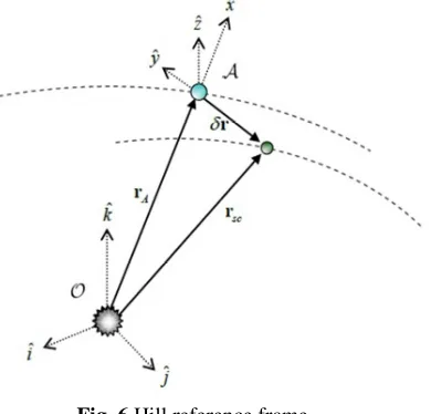
[image:10.595.211.406.179.366.2]x,y and z are the coordinates of the spacecraft with respect to the asteroid in the Hill reference frame, as shown in Fig. 6,and aI and bI are the axes of the ellipsoid (the asteroid is assumed to be a rotation ellipsoid),.
Fig. 6 Hill reference frame
The asteroid is assumed to be spinning around the z-axis with angular velocity ωA. θA is the elevation of the spot
over the y-axis. The model also assumes that all the particles impacting the mirror condense and stick to it. The variation of the thickness of the contamination layer on the mirror is thus computed as:
exp
2
cos
cond
vf layer
v
dh
dt
ρ
ψ
ρ
=
(28)where the layer density ρlayer is 1 g/cm3. The speed of the ejecta is multiplied by 2 to account for the gas expansion in
a vacuum. ψvf is the view factor taken as the angle between the normal of the mirror and the incident flow of gas.
Finally, the power irradiated on the asteroid’s surface is multiplied by a degradation factor τ:
(
)
exp
2
h
condτ
=
−
η
(29)where η=104 cm-1 is the absorption coefficient for Forsterite.
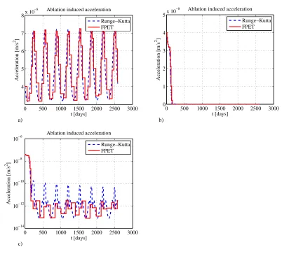
Fig. 7 Typical acceleration profile: a) without contamination b) with contamination c) with contamination
(semi-logarithmic scale)
Fig. 7a shows a typical acceleration profile computed without considering the contamination of the mirror. The figure compares the profile obtained from numerical integration of the trajectory and ablation models with a high order Runge-Kutta method, with the one obtained with analytical propagation with FPET. The periodic behaviour is due to NEO’s motion around the Sun which accounts for oscillations in the solar flux captured by the primary mirror. The two integrations are in good agreement and the difference is due to Eq. (6). Fig. 7b and Fig. 7c show the same case but with the introduction of the contamination model in (Vasile and Maddock 2010). One can see that the amplitude of the acceleration oscillation decreases by more than two orders of magnitude already during the first revolution around the Sun and then stabilises at around 10-11-10-13 m/s2 for the rest of the trajectory.
From Fig. 7 it is important to observe that the FPET propagation approximates very accurately the acceleration profile when its magnitude is high during the first revolution and less correctly when it is decayed for the remainder of the trajectory. This will not affect the accuracy on the computation of the impact parameter since the contribution of the first part will be much more relevant than the second, which will be almost negligible.
As will be detailed in Section 5.1, from an analysis of the literature on NEO, one can observe a considerable variability of the physical parameters of asteroids, in particular Esub, Tsub, cA, kA and ρA, which are at the same time
quite controversial and very critical to the laser ablation system design.
All these sources of uncertainty are of epistemic nature as they correspond to the present lack of knowledge on the asteroid physical properties. Due to the nature of the uncertainty, probability theory would be inadequate to model and quantify its value, therefore it is here proposed to use Evidence Theory to build a correct uncertainty model and introduce it in the combined optimal design of the deflection and spacecraft system.
0 500 1000 1500 2000 2500 3000 4
5 6 7 8x 10
−8 Ablation induced acceleration
t [days]
Acceleration [m/s
2 ]
Runge−Kutta FPET
0 500 1000 1500 2000 2500 3000 0
1 2 3 4 5x 10
−8 Ablation induced acceleration
t [days]
Acceleration [m/s
2]
Runge−Kutta FPET
0 500 1000 1500 2000 2500 3000 10−14
10−12 10−10 10−8 10−6
Ablation induced acceleration
t [days]
Acceleration [m/s
2 ]
Runge−Kutta FPET
b) a)
[image:11.595.313.490.118.281.2]5. Uncertainty Quantification
Evidence Theory, or Dempster-Shafer Theory, is a mathematical framework to model epistemic uncertainty and can be interpreted as a generalisation of classical probability theory (Klir and Smith 2001). In this sense, Evidence theory, is able to model both aleatory (i.e. related to stochastic processes) and epistemic (i.e. due to lack of knowledge) uncertainties. Differently from probability theory, where a probability distribution is used, in Dempster-Shafer theory an uncertain parameter u1 can be modelled with one or more uncertain intervals Ui1, each with its
associated confidence level, also defined as Basic Probability Assignment (BPA):
{
}
1 1
:
1[
1,
1] ;
(
1) [0,1]
i i
i i
U
= ∀
u u
∈
u
u
BPA U
∈
(30)Moreover, while in a standard probability distribution the integral over its domain of existence should be equal to one, the equivalent condition in Evidence Theory is less strict:
1 1 1
,
(
i)
(
i j)
1
i i j
BPA U
+
BPA U
∪
U
=
∑
∑
(31)which translates into the fact that the intervals can not only be disconnected, but also overlapping. When dealing with multiple uncertain parameters, the uncertain space is defined by the Cartesian product of the single mono-dimensional uncertain intervals. A single multimono-dimensional box, whose edges are the uncertain intervals for each uncertain parameter, is called focal element and its BPA is computed as:
(
)
(
1,
2[
1i,
1i] [
2j,
2j]
)
(
1[
1i,
1i]
)
(
2[
2j,
2j]
)
BPA u u
∈
u u
×
u
u
=
BPA u
∈
u u
⋅
BPA u
∈
u
u
(32) Evidence theory also uses two complementary quantities to measure the cumulative confidence, or belief, in a given proposition: Belief and Plausibility. To explain their meaning, let us consider a performance parameter y which is a function f of the design parameters x and of the uncertain parameters u. The set of all y which are below a certain threshold ν is defined as:{
:
( , )
,
,
}
v
Y
=
y y
=
f
x u
<
v
x
∈
D
u
∈
U
(33)then the Belief and Plausibility associated to the proposition y<ν are:
( )
(
)
( )
(
)
B
P
j v
j I
j v
j I
Bel Y
BPA U
Pl Y
BPA U
∈ ∈
=
=
∑
∑
(34)with
{
}
{
}
1
1
:
( )
:
( )
0
j
B v
j
P v
I
j U
f
Y
I
j U
f
Y
− −
=
⊂
=
∩
≠
(35)It should be noted that IB is always a subset of IP, i.e.
I
B⊆
I
P and in this sense Belief and Plausibility can be interpreted as respectively the lower and upper boundary for the likelihood of an event. Differently from the probability of an event and its opposite, Belief and Plausibility are not strictly complementary. Instead the following relationships apply:( )
( )
( )
( )
( )
( )
1
1
1
Bel A
Bel A
Pl A
Pl A
Bel A
Pl A
+
≤
+
≥
+
=
(36)
5.1 Construction of the Uncertain Intervals
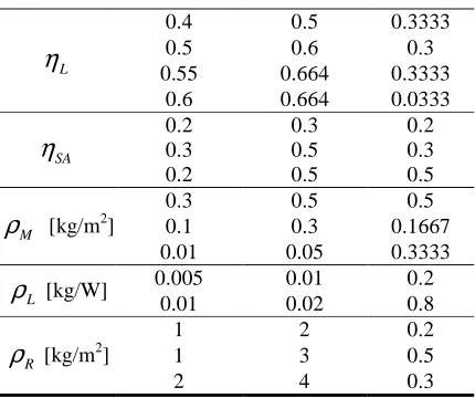
In this section, the uncertain intervals and the associated BPA for each uncertain parameter are defined. Moreover, it will be simulated the situation in which the estimates about the uncertain intervals and their associated confidence come from different sources. In order to do this, in this study the assumption is that the values of uncertain physical and technological parameters stem from the opinion of three different experts, as reported in Table 2, Table 3 and Table 4. Each expert expresses its own opinion on the uncertain intervals and assigns a personal confidence level to each of them. The confidence level represents the perception that experts have in their own level of knowledge. The opinions of the three experts could also be in disagreement with each other. This disagreement can be manifold. In the first instance, the experts can have different opinions on the amplitude of the interval itself and therefore propose slightly different boundaries. Secondly, even if the intervals proposed by different experts are the same, they can associate to them a different confidence and therefore estimate different BPAs. Moreover, some experts can also give a very generic indication that the given parameter can oscillate between a minimum and maximum value with equal confidence, which corresponds to giving a single wide interval with BPA equal to 1. And last, the expert can have no opinion at all on some quantities.
For the technological parameters
η
L,η
SA,ρ
R,ρ
L andρ
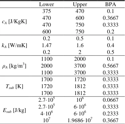
M, the three experts behaves as follows. Regarding the laser efficiency, expert a in Table 2 is rather conservative and assigns a high confidence of 70% to the proposition that the efficiency will be between 40% and 50%; he/she is less confident about the possibility of achieving efficiencies comprised between 50% and 60% and therefore the related probability assignment is 30%. Expert b, in Table 3, on the other hand is probably more realistic and assigns only 30% confidence to the interval of 40-50% efficiency, while giving 60% to the 50-60% efficiency interval and finally introducing another interval between 60% and 66.4% with a confidence of 10%. Expert c, in Table 4, is very optimistic about future developments of lasers and therefore assigns 100% confidence to the statement that lasers could reach efficiencies between 55% and 66.4%. For the laser specific mass, expert a gives 40% confidence about the specific mass being comprised between 0.005 and 0.01 kg/W while is more oriented towards higher specific masses in the interval of 0.01-0.02 kg/W and therefore assigns 60% confidence to the latter. Expert b, on the other hand, is convinced that lightweight laser systems are possible and therefore assign 100% to the 0.01-0.02 kg/W. Expert c does not give any opinion on this topic (reported as n/a in the table). For the solar array efficiency, expert a is again rather sceptical and proposes only one interval between 20% and 30%, obviously with 100% confidence. Expert b suggests only a 40% confidence for the 20-30% efficiency range and instead assigns a 60% confidence about achieving higher efficiencies comprised between 30% and 50%. Expert c again doesn’t express any opinion on the topic (reported as n/a in the table). Regarding the mirror specific mass, expert a is equally oriented towards values between 0.1 and 0.3 kg/m2 and 0.3 and 0.5 kg/m2, therefore confidence will be 50% for both. Expert b again proposes only one interval with 100% confidence for values ranging from 0.3 and 0.5 kg/m2. Expert c instead is very optimistic about the development of lightweight mirrors with specific masses between 0.01 and 0.05 kg/m2. Finally for the radiator, expert a suspects that radiator specific mass will be higher for large radiators like those envisioned for laser ablation spacecraft and therefore suggests 40% for values comprised in the 1-2 kg/m2 and 60% for values between 2 and 4 kg/m2. Expert b doesn’t give an opinion on the topic (reported as n/a in the table) while expert c gives a generic indication that the mirror specific mass will surely be between 1 and 3 kg/m2.As already pointed out in Section 4, physical properties can differ considerably from one asteroid to the other. At the same time, different sources report different physical parameters for the same asteroid. Moreover, data is currently limited to ground based observations and a limited number of fly-by missions to only a few NEOs, such as Eros, Itokawa, Steins and Lutetia. However, these missions demonstrated that the fundamental nature, composition and geometries of NEOs are highly variable. Any generic group of physical characteristics can introduce a significant error within the analysis. Furthermore substantial error bars in Tsub, cA, kA and ρA also exist from the
values between 500 and 600 J/(kg·K), which are typical of Olivine-based S type asteroid but also of M and C types such as Lutetia and Mathilde. It is interesting to note, however, that in some cases like the E type asteroid Steins the estimates can range from 470 up to over 750 J/(kg·K). Thus, expert a suggests two uncertain intervals: the first from 375 to 470 J/(kg·K) with 30% confidence, and the second one from 470 to 600 J/(kg·K) with 70% confidence. Also expert b proposes this latter range, but with 40% confidence only. He also proposes a higher interval from 600 up to 750 J/(kg·K) with 60% confidence. Expert c gives a generic indication that the specific heat will be between 470 and 750 J/(kg·K). For the thermal conductivity, the range spans two orders of magnitude: for common S-type, Olivine bodies and for some E type asteroids it is around 1.47-1.6 W/(m·K); it is as low as 0.2 W/(m·K) for others like M-type Lutetia and C-type Mathilde. In this sense, expert a assigns 20% confidence to an interval to a low interval for relatively rare M/C-type bodies with conductivities comprised between 0.2 and 0.5 W/(m·K). On the other hand, he/she gives 80% to the assumption that the conductivity will be between 1.47 and 1.6 W/(m·K). Expert b is again rather generic giving just a minimum of 0.2 W/(m·K) and maximum of 2 W/(m·K). Expert c is unable to give an opinion (reported as n/a in the table). Regarding the density, sources report values comprised between 1100 and 2000 kg/m3 for most C-type asteroids, and between 2000 and 3700 kg/m3 for S-types and some M-type ones. According to this, expert a thinks that S-type objects will be more common and therefore assigns 70% to the latter interval and 30% to the former. This time too, expert b is very vague, giving indications of a lower bound at 1100 kg/m3 and an upper at 3700 kg/m3. Expert c disagrees with the lower limit and sets it at 2000 kg/m3 instead. Finally, the sublimation temperature shows a more limited variability, with values around 1700 K for S-type and up to 1812 K for other examples. This small variability is also reflected in the experts’ opinion, since expert a assumes the values related to S-type asteroids, between 1700 K and 1720 K, with 100% confidence. Expert b proposes a range spanning 1720-1812 K, again with 100% confidence, while expert c proposes a wider range from 1700 K to 1812 K.
The three sources of information are data-fused following a similar procedure to the one described by Oberkampf and Helton (2002). As a representative example, the procedure is here applied to the data-fusion of the estimates concerning the laser efficiency. As already discussed, the opinions given by three experts are:
a. Conservative opinion: “The Laser efficiency will be between 40% and 50% with 70% confidence and between 50% and 60% with 30% confidence”.
b. Realistic opinion: “The Laser efficiency will be between 40% and 50% with 30% confidence, between 50% and 60% with 60% confidence and between 60% and 66.4% with 10% confidence”.
c. Optimistic opinion: “The Laser efficiency will be between 55% and 66.4% with 100% confidence”. These statements, in mathematical terms can be written as:
a.
[
]
( )
[
]
( )
1 1
2 2
0.4, 0.5
0.7
0.5, 0.6
0.3
a a
a a
U
BPA U
U
BPA
U
=
=
=
=
b.
[
]
( )
[
]
( )
[
]
( )
1 1
2 2
3 3
0.4, 0.5
0.3
0.5, 0.6
0.6
0.6, 0.664
0.1
b b
b b
b b
U
BPA U
U
BPA U
U
BPA U
=
=
=
=
=
=
c. c
U
=
[
0.55, 0.664
]
BPA U
( )
c=
1
Then, to represent and then combine the data given by the three experts, for each of them a matrix is constructed as follows (Oberkampf and Helton 2002):
1. First, one has to list all the possible values the experts propose as lower and upper boundaries for the uncertain intervals. In this case the lower boundaries are
[
0.4
0.5
0.55
0.6
]
and upper boundaries are[
0.5
0.6
0.664
]
.0.4 0.5 0.55 0.6
0.5 0.7 0 0 0
0.6 0 0.3 0 0
0.664 0 0 0 0
In the present case, the three matrices are as follows.
a.
0.7
0
0
0
0
0.3 0
0
0
0
0
0
a
A
=
b.0.3
0
0
0
0
0.6
0
0
0
0
0
0.1
b
A
=
c.0
0 0
0
0
0 0
0
0
0 1
0
c
A
=
At this point the three sets of intervals can be combined into a single one by computing the weighted average of matrices as:
3
a a b b c c
k A
k A
k A
A
=
+
+
(37)where ka, kb, and kc are weights which can be defined arbitrarily in order to give different influence to each source of
information. In this case, all sources are given the same importance and therefore the weights are all set to 1. The resulting matrix is therefore:
0.3333
0
0
0
0
0.3
0
0
0
0
0.3333 0.0333
A
=
from which one derives the uncertain intervals as:
[
]
( )
[
]
( )
[
]
( )
[
]
( )
1 1 2 2 3 3 4 40.4, 0.5 0.3333
0.5, 0.6 0.3
0.55, 0.664 0.3333
0.6, 0.664 0.0333
U BPA U
U BPA U
U BPA U
U BPA U
= =
= =
= =
= =
[image:15.595.126.391.100.322.2]A similar procedure was followed for the remaining nine uncertain parameters, leading to the results reported in Table 5 and Table 6. Note that information fusion of different sources for this specific case is still an open problem. The use of a weighted average is only one possibility. A thorough analysis of the right information fusion technique is out the scope of this paper and will be addressed in future works.
Lower Upper BPA Lower Upper BPA
cA [J/KgK]
375 470 0.3
L
η
0.4 0.5 0.7470 600 0.7 0.5 0.6 0.3
kA [W/mK]
0.2 0.5 0.2
SA
η
0.2 0.3 11.47 1.6 0.8
ρA [kg/m3]
1100 2000 0.3
M
ρ
[kg/m2] 0.1 0.3 0.52000 3700 0.7 0.3 0.5 0.5
Tsub [K] 1700 1720 1
ρ
L [kg/W]0.005 0.01 0.4 0.01 0.02 0.6 Esub [J/kg] 2.7·105 6·106 1
R
2 4 0.6
Table 2 Uncertain parameters estimates from expert a
Lower Upper BPA Lower Upper BPA
cA [J/KgK]
470 600 0.4
L
η
0.4 0.5 0.3600 750 0.6 0.5 0.6 0.6
0.6 0.664 0.1
kA [W/mK] 0.2 2 1
η
SA0.2 0.3 0.4 0.3 0.5 0.6
ρA [kg/m3] 1100 3700 1
ρ
M[kg/m
2] 0.3 0.5 1
Tsub [K] 1720 1812 1
ρ
L [kg/W] 0.01 0.02 1Esub [J/kg]
2.7·105 106 0.2
R
ρ
[kg/m2] n/a [image:16.595.136.465.327.446.2]107 1.9686·107 0.8
Table 3 Uncertain parameters estimates from Expert b
Lower Upper BPA Lower Upper BPA
cA [J/KgK] 470 750 1
η
L 0.55 0.664 1kA [W/mK] n/a
η
SA n/aρA [kg/m3] 2000 3700 1
ρ
M[kg/m
2] 0.01 0.05 1
Tsub [K] 1700 1812 1
ρ
L [kg/W] n/aEsub [J/kg]
4·106 6·106 0.7
R
ρ
[kg/m2] 1 3 1 [image:16.595.192.406.474.686.2]107 1.9686·107 0.3
Table 4 Uncertain parameters estimates from Expert c
Lower Upper BPA
cA [J/KgK]
375 470 0.1
470 600 0.3667
470 750 0.3333
600 750 0.2
kA [W/mK]
0.2 0.5 0.1
1.47 1.6 0.4
0.2 2 0.5
ρA [kg/m3]
1100 2000 0.1
2000 3700 0.5667
1100 3700 0.3333
Tsub [K]
1700 1720 0.3333
1720 1812 0.3333
1700 1812 0.3333
Esub [J/kg]
2.7· 105 106 0.0667
2.7· 105 6·106 0.3333
4· 106 6·106 0.2333
107 1.9686·107 0.3667
Table 5 Uncertain intervals of NEO physical properties
L
η
0.4 0.5 0.3333
0.5 0.6 0.3
0.55 0.664 0.3333
0.6 0.664 0.0333
SA
η
0.20.3 0.30.5 0.20.30.2 0.5 0.5
M
ρ
[kg/m2]0.3 0.5 0.5
0.1 0.3 0.1667
0.01 0.05 0.3333
L
ρ
[kg/W] 0.005 0.01 0.20.01 0.02 0.8
R
ρ
[kg/m2]1 2 0.2
1 3 0.5
[image:17.595.191.406.101.281.2]2 4 0.3
Table 6 Uncertain intervals of technological parameters
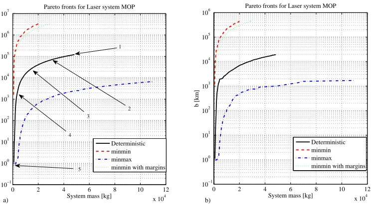
6. Multi Objective Optimization Under Uncertainty
Once the uncertainties on system design and asteroid physical characteristics are defined, one can try to find the optimal design of the deflection system under uncertainty. The performance, i.e. the achieved deviation, needs to be maximised while minimising a measure of the cost of the mission, e.g. the mass into space. According to the spacecraft system model presented in previous sections, performance and cost can be optimised with respect to four design parameters: the diameter of the primary mirror dM, the number of spacecraft nsc, the warning time twarn (time
from the beginning of the deflection action to the time of the expected impact with the Earth) and the concentration ratio Cr. The performance measure to be maximised is the impact parameter b, while the cost measure to be
minimised is the total mass of the formation msys. This leads to a classical multiobjective optimisation problem. The
impact parameter is computed by means of the deflection and ablation model detailed in Sec.2 and Sec.4 while the total system mass is derived as in Sec.3.
As a first step one can determine the set of Pareto optimal solutions for a fixed value of the uncertain parameters L
η
,η
SA,ρ
R,ρ
L,ρ
M, Esub, Tsub, cA, kA and ρA. Their value was chosen according to the available literature (Britt et al. 2002; Pieters and McFadden, 1994; Price 2004) and are reported in Table 7. Moreover, since at this stage uncertainties are not yet accounted for with Evidence theory, system margins as in Table 1 are included in the model, in order to replicate the standard system engineering method to deal with uncertainty.
NEO Physical properties Technological parameters Parameter Value Parameter Value
cA [J/KgK] 750
η
L 0.6kA [W/mK] 2
η
SA 0.41ρA [kg/m3] 2600
ρ
M [kg/m 2] 0.1
Tsub [K] 1800
ρ
L [kg/W] 0.005 Esub [J/kg] 5·106ρ
R [kg/m2
[image:17.595.187.410.516.630.2]] 1.4
Table 7 Set of fixed values for uncertain parameters
The multi objective optimisation problem to be solved is:
( )
( )
min
system,
,
D
m
b
∈
−
x
x u
x u
(38) where x is the design parameter vector comprising x=[dM, nsc, twarn, Cr]T, for which the boundaries are in Table 8, and
Lower Upper
dM [m] 2 20
nsc 1 10
twarn [yrs] 1 8
[image:18.595.185.410.116.176.2]Cr 1000 3000
Table 8 Boundaries for optimization parameters
Note that the presence of the discrete variable nsc makes this a mixed integer-nonlinear multiobjective
optimisation problem. The optimisation problem is solved with MACS, a hybrid memetic stochastic algorithm (Vasile and Zuiani 2011).
When epistemic uncertainties are introduced through Evidence Theory the MOO problem (38) has to be reformulated in order to maximise the Belief in the optimal value of impact parameter and total system mass. Formally problem (38) would translate into the MOO under uncertainty:
max
(
( , )
)
max
(
( , )
)
min
min
b D
sys m
D
b
m
Bel
b
Bel m
ν
ν
ν
ν
∈ ∈−
<
<
x
x
x u
x u
(39)
The solution of problem would require the computation of the Belief value for different design parameters and for different values of the thresholds νb and νm for all possible values of the uncertain parameters u within the uncertain space U: for each x, set (33) needs to be computed for each of the functions b and msys for different νb and
νm respectively and the cumulative functions (34) need to be independently computed for both b and msys.. The identification of the set (33) would need the computation of the max and min of b and msys over all the focal elements in U. However, the number of focal elements in U is an exponential function of the number of uncertain parameters (Vasile and Croisard 2010) which translates into an exponentially increasing number of optimisation problems required to compute the cumulative quantities in (34). In practise, however, the full Belief and Plausibility curves are not required and one can study only the worst and best case scenarios.
The best case scenario corresponds to the design, uncertainty vectors and thresholds that yield a Plausibility equal to 0. Below this value of the thresholds the deflection mission is not possible assuming the available body of knowledge of spacecraft systems and asteroid physical properties. The worst case scenario corresponds to the design, uncertainty vectors and thresholds that yield a Belief equal to 1. Above this value of the thresholds the mission is certainly possible, given the current body of knowledge, but would be suboptimal.
The optimal design vector and thresholds that yield a Belief equal to 1 for all possible u in U can be computed solving the following multiobjective minmax problem:
( )
(
( )
)
min max
system,
max
,
D U
m
Ub
∈ ∈ ∈
−
x u
x u
ux u
(40) In fact, for a given x, the minimum possible threshold value corresponds to the maximum value of msys and –b over the whole uncertain space U, for which boundaries are reported in Table 5 and Table 6. Because the focal elements in U can be overlapping or can be disconnected, the identification of the maximum of msys and –b might be problematic as one would need to explore each focal element independently and therefore face an exponential number of optimisation problems. In order to avoid this exponential complexity, all focal elements are collected, through an affine transformation, into the unit hypercube
U
such that they are not overlapping or disconnected.The optimal design vector and thresholds that yield a Plausibility equal to zero for all possible u in U can be computed by solving the following multiobjective minmin problem:
( )
(
( )
)
min min
system,
min
,
D U
m
Ub
∈ ∈ ∈
−
x u
x u
ux u
(41)Again as before the focal elements are mapped into the unit hypercube
U
and the search is run overU
. Note that, differently from the case of problem (38), system design margins are no longer needed and therefore the values for kdry, kS, kM, kL are all set to 1.multiobjective minmin/minmax problems. The standard MACS framework is used to explore the design space D and solve the minimisation problem, i.e. generate new candidate design vectors xc and select the ones that minimise the
vector function:
( )
max
(
,
)
max
(
(
,
)
)
T
c system c c
U
m
Ub
∈ ∈
=
−
u u
J x
x u
x u
(42)The value of each component of the vector function J is the result of a single objective maximisation over the space of the uncertain parameters.
The maximisation subproblems in (42) are solved by running an evolutionary algorithm based on Inflationary Differential Evolution (IDEA) (Vasile et al. 2011a) for a fixed number of function evaluations. MACS was run for 30000 function evaluations with 10 individuals, of which 2 are explorers and perform a local search (see Vasile and Zuiani 2011 for details). The sub-cycles with IDEA where run for 250 function evaluations with 5 individuals. These settings were devised after a series of preliminary tests. The solution of problems (40) and (41) provides the intervals for both the performance and the design parameters. In particular, the worst case corresponds to the maximum Belief condition:
( )
(
( )
)
[ , ]
arg min max
,
max
,
( )
1
system
D U
m
Ub
Bel
∈ ∈ ∈
=
=
−
=
x u u
y
x u
x u
x u
y
(43)
The best case instead corresponds to the minimum Plausibility point:
( )
(
( )
)
[ , ]
arg min min
,
min
,
( )
0
system
D U
m
Ub
Pl
∈ ∈ ∈
=
=
−
=
x u u
y
x u
x u
x u
y
(44)
As a comparison, a minmin problem analogous to (44) is solved with the reintroduction of system design margins. Finally the 4 optimisation problems are considered both in the case with and without the contamination are solved. In summary, a total of 8 Pareto curves are generated, 4 each for the cases with and without the contamination:
1. deterministic, i.e. a bi-objective optimisation problem on
x
∈
D
as in (38). The system model does include the margins specified in Table 1 and constant values for uncertain parameters u are used as in Table 7. The problem is solved with the standard MACS.2. minmax, bi-objective optimisation problem as in (40). The system model doesn’t include margins. The problem is solved with the modified MACS.
3. minmin, bi-objective optimisation problem as in (41). The system model doesn’t include margins. The problem is solved with the modified MACS.
4. minmin with margins, bi-objective optimisation problem as in (41). It’s analogous to the previous one but this time the system model does include the margins specified in Table 1. The problem is solved with the modified MACS.