Methods for the calculation of aerodynamic models for flight simulation

(1)

Methods for the Calculation of Aerodynamic Models for

Flight Simulation

Thesis submitted in accordance with the requirements of the University of Liverpool for the degree of Doctor in Philosophy

by

Andrew McCracken (BEng)

(2)

(3)

Copyright c2014 by Andrew McCracken

(4)

(5)

A model is a caricature that overemphasizes some features at the expense of others.

(6)

(7)

Abstract

Flight dynamics analysis using computational models is a key stage in the design of aircraft. The models used in industry consist of two main parts. The first is a tabular aerodynamic model which is essentially a large database of aerodynamic data. The tab-ular aerodynamic model is a highly dimensional database containing aerodynamic loads and moments for different parameter combinations. In order to reduce the size of the tables, a number of assumptions are made. These include having sufficient resolution of the parameter space to capture the variation in the flow dynamics; decoupling certain parameters to reduce the dimensionality; using a single dynamic derivative, assuming independence from the flow conditions; and finally neglecting flow history effects which are dominant during manoeuvres with highly unsteady flow phenomena.

Secondly is the use of dynamic derivatives to simulate unsteady motion effects. These are calculated using small–amplitude forced oscillatory motions. In order to ac-celerate their computation, frequency domain methods are used. The Linear Frequency Domain and Harmonic Balance are two such methods used in this work. As part of the frequency domain calculations, linear solvers are used to provide solution to the frequency domain problem. These solvers use preconditioners to accelerate the time to solution. An alternative method of preconditioning is proposed in this work based on the first and second order spatial discretisation Jacobian matrices. It is shown that there is significant speed up achieved by varying the proportions of the first and second order terms in the preconditioner matrix.

(8)

(9)

Acknowledgements

I would firstly like to thank my supervisors Professor Ken Badcock and Professor George Barakos for making it possible to carry out this work. Also to my examiners Dr Dorian Jones and Dr Mark White for their time in examining this thesis and for their input on improvements. As always, thanks must go to all those in the CFD lab past and present for making each day survivable and always a good laugh. The extra guidance from Dr Andrea Da Ronch, Dr Sebastian Timme and Dr David Kennett were invaluable in overcoming numerous problems, both intellectually and politically.

Thanks must also go to the Engineering and Physical Sciences Research Council (EPSRC) and Airbus Ltd for their funding of this project. Also, to the Flight Physics department at Airbus Filton for their input throughout. Further to this, the help of staff in DLR’s Institute of Aerodynamics and Flow Technology, particularly Markus Widhalm, was invaluable in the work on the Linear Frequency Domain.

(10)

(11)

Declaration

I confirm that the thesis is my own work, that I have not presented anyone else’s work as my own and that full and appropriate acknowledgement has been given where reference has been made to the work of others.

(12)

(13)

List of Publications

Da Ronch, A., McCracken, A., Badcock, K.J., “Assessing the Impact of Aerodynamic Modelling on Manoeuvring Aircraft,” AIAA Science and Technology Forum and

Exposition 2014, National Harbor, MD, 13–17 Jan 2014.

McCracken, A., Badcock, K.J., “Uncertainty Quantification in Flight Dynamics Modelling,” ECCOMAS Young Investigators Conference 2013, Bordeaux, 2–6 Sept 2013.

McCracken, A., Kennett, D.J., Badcock, K.J., “Assessment of Tabular Models Using CFD,”AIAA Atmospheric Flight Mechanics Conference, Boston, 19–22 Aug 2013.

Da Ronch, A., McCracken, A., Badcock, K.J., Widhalm, M., and Campobasso, M.S., ”Linear Frequency Domain and Harmonic Balance Predictions of Dynamic Derivatives,” Journal of Aircraft, Vol. 50, No. 3, pp 694–707, 2013.

McCracken, A., Da Ronch, A., Timme, S., Badcock, K.J., “Solution of Linear Systems in Fourier-Based Methods for Aircraft Applications,” International Journal

of Computational Fluid Dynamics, Vol. 27, No. 2, pp 79–87, 2013.

McCracken, A., Akram, U., Da Ronch, A., Badcock, K.J., “Requirements for Com-puter Generated Aerodynamic Models for Aircraft Stability and Control Analysis,“5th

Symposium on Integrating CFD and Experiments in Aerodynamics, Tokyo, October

2012.

McCracken, A., Timme, S., Badcock, K.J., ”Accelerating Convergence of the CFD Linear Frequency Domain Method by a Preconditioned Linear Solver,“ ECCOMAS 2012, Vienna, September 2012.

Da Ronch, A., McCracken, A., Badcock, K.J., Ghoreyshi, M., and Cummings, R.M., “Modeling of Unsteady Aerodynamic Loads,” AIAA–2011–2376, AIAA Atmospheric

(14)

(15)

List of Figures

1.1 Flow conditions of interest . . . 3

2.1 Unit cube control volume [1] . . . 13

2.2 Regular grid and associated dual-cells . . . 16

2.3 Point cloud with ellipse . . . 17

2.4 NACA 0012 aerofoil point distribution with underlying structural model 18 3.1 NACA 0012 grids . . . 32

3.2 NACA 64A010 grid . . . 33

3.3 SDM grid . . . 33

3.4 Goland wing grids . . . 34

3.5 LANN wing grid . . . 34

3.6 NACA0012 fine AGARD CT2 solution comparison . . . 36

3.7 NACA0012 fine AGARD CT5 solution comparison . . . 36

3.8 Convergence comparison . . . 38

3.9 Parallel performance (Goland Euler) . . . 41

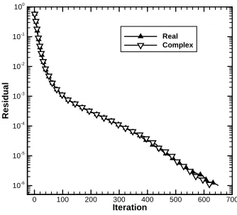
3.10 Real vs Complex solver convergence (Goland Euler) . . . 42

3.11 Second order preconditioner comparison . . . 43

3.12 First order preconditioner . . . 44

3.13 Weighted preconditionerα= 0.90 . . . 44

3.14 Influence of preconditioner weighting on convergence . . . 45

3.15 Convergence and Real Positive eigenvalue (NACA 0012 fine AGARD CT2) 46 3.16 Error from exact solution (NACA 0012 fine AGARD CT2) . . . 47

3.17 Pitching moment coefficient (NACA 0012 fine AGARD CT2) . . . 48

3.18 NACA 0012 point distributions . . . 49

3.19 Pitching moment coefficient loops from PML HB . . . 49

3.20 Speed up of PML HB . . . 50

4.1 CFD validation (McCroskey case 8) . . . 54

4.2 NACA 0012 RANS point distribution . . . 55

4.3 Ramp manoeuvre replay 2◦ /s . . . 56

(18)

4.5 Oscillatory manoeuvre replays . . . 57

4.6 NACA 0012 point distributions . . . 58

4.7 NACA 0012 point distributions with underlying structure . . . 59

4.8 Ramp motion at 10◦ /s . . . 60

4.9 Pressure coefficient distribution at two locations in the manoeuvre at Mach 0.8 . . . 62

4.10 Pressure coefficient distribution at an incidence of -2.0◦ in the manoeuvre at Mach 0.8 . . . 62

4.11 Obstacle avoidance manoeuvre(Euler) . . . 64

4.12 Obstacle avoidance manoeuvre (RANS) . . . 65

4.13 LANN wing grid . . . 67

4.14 LANN wing replay comparison . . . 67

5.1 Effect of resolution on lift coefficient prediction for aerofoil with control surface at Mach 0.8 . . . 71

5.2 Effect of input parameters in pitch damping derivative . . . 72

5.3 Aerofoil with control surface ramp replays with and without coupling . . 73

5.4 Aerofoil with control surface obstacle replays with and without coupling in the derivative . . . 75

5.5 LANN Wing: coupled and decoupled replays . . . 76

5.6 Aerofoil table resolution comparison . . . 78

5.7 LANN table resolution comparison . . . 79

5.8 Aerofoil: Effect of dynamic derivative value on replay . . . 80

5.9 LANN Wing: Effect of dynamic derivative value on replay . . . 81

5.10 Oscillatory manoeuvre replays with quasi-steady . . . 82

5.11 Turbulent eddy viscosity at 19.24◦ on the upstroke . . . 83

5.12 Turbulent eddy viscosity at 10.0◦ on the downstroke . . . 84

5.13 Effect of history on the replay . . . 85

5.14 Two degree of freedom aerofoil [2] . . . 86

5.15 Free–response control inputs . . . 87

5.16 Tabular replays with and without coupling . . . 88

5.17 Table resolution comparison . . . 88

5.18 Effect of pitch damping derivative value on replay . . . 89

5.19 Lift damping derivative variation with flight parameters . . . 90

5.20 M = 0.3, α0 = 0.0◦,αA = 5.0◦, k = 0.001 . . . 92

5.21 M = 0.3, α0 = 0.0◦,αA = 5.0◦, k = 0.1 . . . 93

5.22 M = 0.3, α0 = 8.0◦,αA = 5.0◦, k = 0.001 . . . 93

(19)

List of Tables

2.1 Example Aerodynamic Table (x indicates non-zero entry) . . . 20

3.1 AGARD test case conditions (Euler) . . . 32

3.2 Solver Parameters . . . 35

3.3 Solver speed test results . . . 37

3.4 PETSc option test cases . . . 38

3.5 PETSc option test results NACA 0012 AGARD CT2 . . . 39

3.6 Solver memory requirement . . . 40

3.7 Solver memory requirement relative to steady state . . . 40

3.8 Augmentation comparison (Goland Euler) . . . 42

3.9 TAU-HB memory requirement (NACA 0012 fine AGARD CT2) . . . 48

3.10 PML-HB memory requirement (MB) . . . 50

4.1 Example Aerodynamic Table (x indicates non-zero entry) . . . 51

4.2 Reduced table for Mach and incidence . . . 52

4.3 Reduced table for Mach and control surface deflection . . . 52

4.4 Control surface ramp manoeuvre parameters . . . 60

4.5 Control surface obstacle manoeuvre parameters . . . 63

4.6 LANN wing manoeuvre parameters . . . 66

5.1 Coupled Aerodynamic Table (x indicates non-zero entry) . . . 69

5.2 Decoupled Aerodynamic Table for sideslip (x indicates non-zero entry) . 69 5.3 Decoupled Aerodynamic Table for control surface deflection (x indicates non-zero entry) . . . 69

5.4 Coupled and decoupled table parameter ranges . . . 72

5.5 LANN coupling manoeuvre parameters . . . 76

5.6 Aerofoil with control surface table resolutions per Mach number . . . . 77

5.7 LANN wing table resolutions per Mach number . . . 78

(20)

(21)

Nomenclature

Symbols ˜

A Approximation of A

A System matrix

Aα Mixed order Jacobian matrix

Af First order spatial accruate fluid Jacobian

As Second order spatial accruate fluid Jacobian

b Right hand side vector

CL,CD,CY Force coefficients (lift, drag, side-force)

CLα Lift-curve slope (1/rad.)

CLq Lift damping derivative (1/rad./s)

Cl,Cm,Cn Moment coefficients (roll, pitch, yaw)

Cmα Pitching moment slope (1/rad.)

Cmq Pitch damping derivative (1/rad./s)

c Chord length (m)

h Plunge height (m)

Iy Moment of inertia about pitch axis (kg.m2)

k Reduced frequency

L Lift force (N)

Lh Change in lift due to heave (N/m)

Lh˙ Change in lift due to heave velocity (N/m/s)

Lα Change in lift due to pitch (N/rad.)

Lα˙ Change in lift due to pitch rate (N/rad./s)

M Mach number

Mh Change in pitching moment due to heave (N.m/m)

M_h˙ Change in pitching moment due to heave velocity (N.m/m/s)

Mα Change in pitching moment due to pitch (N.m/rad.)

Mα˙ Change in pitching moment due to pitch rate (N.m/rad./s)

(22)

m Number of Krylov subspace vectors

NH Number of harmonics retained

P Preconditioner matrix

Pα Preconditioner based on mixed order Jacobian

q Pitch rate (rad./s)

R Residual

r Krylov residual vector

Re Reynolds’ number

t Time (s)

U∞ Free stream velocity (m/s)

¯

w Steady state component

ˆ

w Vector of Fourier coefficients

w Vector of conserved flow variables

˜

w Perturbation component

x Grid point coordinates

˙

x Grid point velocities

Greek Symbols

α, β Angle of attack, Sideslip (◦

)

α0 Mean incidence

∆α Amplitude of oscillation

δele,δail,δrud Control surface deflections (elevator, aileron, rudder) (◦)

ǫ Amplitude factor for finite difference step

ω Reduced circular frequency

Subscripts

α Weight applied to second order Jacobain terms

f First order spatial accuracy

s Second order spatial accuracy

Acronyms

BCSR Block Compressed Sparse Row

CGS Conjugate Gradients

CSR Compressed Sparse Row

GCR Generalised Conjugate Residual

GMRes Generalised Minimal Residual

HB Harmonic Balance

(23)

LFD Linear Frequency Domain

LU Lower Upper

LU-SGS Lower Upper Symmetric Gauss Seidel

NLFD Non-Linear Frequency Domain

PETSc Portable Extensible Toolkit for Scientific Computation

RANS Reynolds Averaged Navier-Stokes

RCM Reverse Cuthill-McKee

SDM Standard Dynamics Model

(24)

(25)

Chapter 1

Introduction

1.1 Computational Aerodynamic Models

Industrial practice is seeing ever increasing use of computer simulations for flight dy-namics analysis. The aerodynamic models used in the simulation must be fit for purpose to ensure reliable results. The tabular aerodynamic model is one such computational model that is used frequently as part of aircraft loads assessment during the design phase, as well as in onboard control systems. Despite the frequent and long term use of this model, it has not been fundamentally assessed for civil domain problems.

Computational models used for flight simulation consist of a number of components. These typically include an aerodynamic database, a method to account for unsteady effects and a method to include the flight mechanics, in order to model the aircraft response for given loads and moments. The aerodynamic database contains the force and moment coefficients for a given parameter set covering the flight envelope, which are obtained by empirical or computational methods. For manoeuvres where the rates become significant, or where the aerodynamics begin to deviate from the linear regime, unsteady modelling is required. A number of approaches have been proposed for this which will be discussed shortly. The final part is that of the flight mechanics modelling. The equations of motion are set up for the given configuration and describe the response of the loads and moments present at each point within the manoeuvre. The manoeuvre is then simulated by stepping through time and moving the aircraft to its new position until a complete trajectory can be traced.

(26)

specif-ically calculating a confidence interval for the predictor, in order to determine where samples should be taken. This approach enables nonlinearities to be better captured in the parameter space by locating high-fidelity simulations in these regions. The second scenario was that of a changing geometry. A data fusion approach was used, whereby the original geometry aerodynamic model was augmented by a few high-fidelity sam-ples for the new configuration. The new aerodynamic model was then used for the new configuration. This approach has the benefit of only requiring a few expensive simulations to obtain an updated model. It was shown that, for the case presented, the required number of samples in the first scenario was reduced from 2000 to 35, and for the second scenario, down to just 10 samples.

Work by Da Ronch et al. [4] used the method described above for further test cases. The focus of this work was on the applicability of the models for flight dynamics simu-lation. Again, a number of aerodynamic models were used with a hierarchy of fidelities as the source of data including high-fidelity CFD. The method was assessed using five different test cases across a range of regimes. All the models were full aircraft of conven-tional and unconvenconven-tional configurations. The performance of the aerodynamic model was compared with wind tunnel and flight test data and it was shown that the model was suitable for the cases presented.

A further study by Mackman et al. [5] looked to the use of surrogate models to reduce the number of samples required to generate an aerodynamic model. In this work, CFD simulations were used as the source of aerodynamic data. Two interpolation approaches were used to create the surrogate models. The first was the same Kriging method used in the previously described studies. The second made use of radial basis functions (RBF). The sample locations were then chosen based on the mean squared error of the interpolant. The two approaches were tested on the DLR-F12 aircraft and an RAE 2822 aerofoil. It was shown that both methods required fewer points to form the aerodynamic model than space-filling techniques.

(27)

This framework was then used by Vallespin et al. in [7]. The assessment was extended to additional test cases, and for a wider range of manoeuvres, with the main focus on the use of an unmanned combat air vehicle (UCAV). This case was designed to cover a large flight envelope, which at high angles of attack, included complex vortical flow adding to the difficulty in modelling the unsteadiness. Again it was seen that there was good agreement across most of the manoeuvres, although when very high rates were present, the tabular model began to breakdown. The fundamental assumptions in the tabular model are mentioned as possible sources of error, although they are not individually assessed.

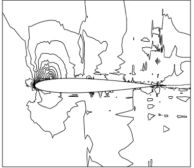
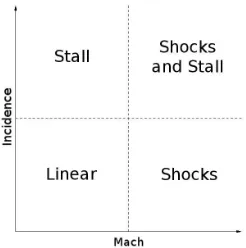
[image:27.595.257.380.373.497.2]

There are a number of examples where the tabular model is no longer adequate but little work has been carried out to assess the fundamental assumptions in the formulation of this model, namely resolution of tables, decoupling parameters, quasi-steady modelling and dynamics modelling. Initial work to assess the assumptions was presented in [8], where an aerofoil case was taken with no control surface to better understand the performance of the tables through a number of regimes as shown in Fig. 1.1.

Figure 1.1: Flow conditions of interest

Manoeuvres in the linear portion of the figure, which was up to around Mach 0.5 and incidence = 10.0◦

for the case used, were well modelled. However, in the shock and stall region, which was the dynamic stall case in the paper, large discrepancies began to show displaying the inadequacy of modelling the time history. The tables used were two–dimensional across a small parameter space, and as a result meant it was not possible to properly assess the other assumptions. Also assessed was the dependence of the value of the dynamic stability derivatives on the Mach number, incidence, amplitude of oscillation and reduced frequency. It was shown that through the linear regime, the dynamic derivatives remained fairly constant in value, although again when there was large unsteadiness, the values began to vary.

(28)

simple was that of the dynamic stability derivative model. This was shown in previous work by the author to be inadequate for combat aircraft manoeuvre simulation. It is however used as the base method to which others are compared. The next approach is that of a Volterra series [11]. This approach is similar to the dynamic derivative method in that it expands the coefficients as a series. However, in the Volterra series, there is a method to account for time history effects in the Volterra kernel. This kernel describes how the output varies with changes in the inputs through time and must be computed using training data. The source of this data can be empirical or computational such as from CFD. A further set of methods come under Indicial approaches [12, 13]. Indicial approaches can be either linear or nonlinear in nature. The linear methods consider the response of an aerodynamic load to be linearly varying with the forcing function. For example, the lift coefficient has a constant variation with the change in incidence. This is limited in its approach due to the variation changing as the aerodynamics become more complex, such as at high angles of attack. This can be worked around by using the nonlinear indicial methods. The difference from the linear method is that the variation of the output with the input is computed for a number of input values. This provides a history of responses. It was shown that the traditional stability derivative approach was not sufficient to capture the unsteady flow phenomena and that the indicial methods were much more suitable.

A further analysis of unsteady modelling approaches with a focus on flight dynamics was carried out in [14], which covered some of those previously mentioned, although extended the work to include the Surrogate-Based Recurrence Framework (SBRF) [15]. The SBRF method requires forming a surrogate model to describe how the outputs, aerodynamic loads and moment, relate to the inputs. The surrogate is formed using a number of CFD solves as training data, with a specific number of historical solu-tions used to describe the variasolu-tions. Increasing the number of historical data points, improves the approximation power of the model. Once the surrogate is formed, the inputs can be prescribed, and the outputs determined easily. The test case was a pitch-ing NACA 0012 aerofoil in the transonic regime. The performance of each method was compared to a time–accurate CFD solution. It was shown that the SBRF model was best able to model the flow phenomena, and at a similar cost to the conventional stability derivative approach.

Although each of the above have their benefits, the most widely used in practice remains the stability derivative model originally proposed by Bryan [16]. This model is based upon the assumption that the load and moment coefficients can be broken down into a steady state component and an unsteady component (i.e. changes in the values are relative to the rate of the motion). The application of this method is discussed later.

(29)

the 1940s used oscillatory wind tunnel tests with various aerofoil cross sections to view the effect of the flight conditions on the dynamic derivatives. It was shown that there can be significant variation with the oscillatory frequency, oscillatory amplitude, mean incidence, location of the axis of oscillation, Reynolds number and the aerofoil profile. It was particularly noted that the pitch damping derivative can vary between negative and positive values with changes in the mean incidence. This is of importance around the stall, where the difference between a damped (negative derivative) and under– damped (positive derivative) system can be significant. Further work was carried out by Greenwell in [18]. In this work, there was a focus on the effect of the oscillatory frequency on the values of the static and dynamic stability derivatives. Again this was done using wind tunnel tests. A delta wing test case was used, where it was shown that the frequency of oscillation can have a significant effect on the dynamic derivative values, particularly at high angles of attack. When a manoeuvre simulation is carried out, a single value for the dynamic derivative is usually taken, which is assumed to be independent of the flight parameters. This is however not the case.

1.2 Frequency Domain Methods

Running full-order time-accurate unsteady CFD calculations to obtain all the dynamic derivative values required for a complete aircraft flight envelope assessment, can be very computationally expensive. The periodicity in the simulations used to compute the derivative values allow the use of frequency domain methods to accelerate the computation time. These were initially developed for turbomachinery flows [19, 20]. The methods have been adapted for use in many areas of aerospace including the prediction of unsteady air loads [21], flutter analyses [22] and on the application of predicting dynamic derivatives for flight dynamics [23]. These methods make use of the periodic nature of certain simulations, to allow a frequency domain representation of the solution. This has the benefit of being able to compute the periodic state directly, without the need to resolve an initial transient. Two methods are used in this work. The first is the Linear Frequency Domain (LFD) method. LFD assumes periodic, small amplitude variations about a steady state, which allows linearisation of the time-accurate flow equations and subsequent solution in the frequency domain. This is described further in Section 2.4.1. The second is the Harmonic Balance (HB) approach which models the flow equations as a Fourier series, and truncates this to a specified number of harmonics. This is described in Section 2.4.2.

(30)

of the incomplete factorisation preconditioner has received attention with many papers being published, although the outcomes are usually only focused on stabilising for a particular type of matrix. In this thesis, a method of stabilisation is explored for general cases arising from CFD problems.

The Linear Frequency Domain method was originally developed for use in turbo-machinery flows by Hall and Crawley [24] as a small disturbance Euler method. This paper set out to address the limitations of linearisation of the unsteady problem, namely the assumptions of isentropy and irrotationality of the flow, to allow shock waves to be accurately predicted. The method was demonstrated using a hyperbolic channel, and a cascade. The results from the cascade are of most interest here, featuring a pitching aerofoil section. The method was compared against incompressible analytical solutions. The method showed very good agreement in the pressure plots with just a little over-estimation in the real and imaginary components of pressure.

The linearized Euler equations have been used for CFD solution. A small distur-bance Euler equations solver which was developed by Kreiselmaier and Laschka in [25], and which was then developed for use with the Navier-Stokes equations by Pechloff and Laschka in [21]. The underlying flow solver was Technische Universit¨at M¨unchen’s FLM Navier-Stokes solver. The method was demonstrated on sinusoidally pitching NACA 64A010 and NLR 7301 aerofoils at AGARD CT8 and CT5 [26] viscous condi-tions respectively. The results from the FLM.SD.NS method were compared against the FLM.NS and FLOWer codes showing good agreement even for the stronger shock dynamics in the CT5 case.

The LFD formulation is derived from the same principles as the small disturbance Navier-Stokes method however, the perturbations are transformed into the frequency domain to allow subsequent solution of a linear system in the form Ax=b. This has been implemented within the DLR TAU-code. It was first presented by Widhalm et al. [22] being demonstrated on both 2D and 3D cases including the full DLR-F12 aircraft model. The method is run on an inviscid subsonic heaving NACA 0012 case, a viscous transonic pitching NACA 64A010 case, the viscous transonic pitching LANN wing and a viscous transonic DLR-F12 full aircraft case. The paper shows very good perfor-mance of the LFD method in terms of predicting the pressure distributions against the RANS calculations for all cases. There are only small discrepancies at large gradients, particularly at the peaks for the LANN wing. A limitation of this method is in the formulation of the right-hand side of the linear system using finite differences which introduces problems when choosing a general finite difference step size. This method is the basis for the work presented in this thesis.

(31)

improve-ment in CPU time is achieved using the LFD method, whilst retaining the main flow features to provide a good estimate of the dynamic derivatives. This paper offers a comprehensive study of the methods for several test cases.

The Harmonic Balance was originally proposed for modelling unsteady nonlinear flows by Hall et al [27]. The purpose of this paper was to solve the Navier-Stokes and Euler equations in Harmonic Balance form to then be able to solve these as a steady state problem when applied to turbomachinery cascade flows. The method involves expanding the flow unknowns in a Fourier series and then retaining a limited number of harmonics. The method is validated on a front stage compressor rotor in viscous transonic conditions with an inflow Mach number of 1.27 and Reynold’s number of 1.35x106_{. The rotor blades undergo a harmonic pitching motion with a reduced}

frequency of 1.0 and pitch amplitudes of 0.01◦

and 1.0◦

. For the smaller amplitude case, it is shown that even using one harmonic is sufficient to represent the flow due to nonlinear effects being very small for this case. The larger amplitude pitch however requires at least three harmonics to represent the flow to within engineering accuracy. The method was found to be between one and two orders of magnitude quicker in terms of CPU time than the equivalent unsteady time-accurate computation.

In [28], an implicit version of the Harmonic Balance technique was described for use in flight dynamics analysis. The purpose of implementing the implicit solver was to speed up the solution time by removing the reliance on explicit convergence acceleration methods such as Multigrid. The new solver is tested using a pitching NACA 0012 aerofoil under AGARD CT1 conditions and a pitching F-5 wing with a wing tip launcher and missile at Mach 0.896, α=0.004◦

, ∆α=0.117◦

andk= 0.275. It was shown that for both cases, one harmonic was sufficient to obtain accurate solutions at certain points in the pressure plots and moment loops, but that accurate reconstruction through the whole cycle required higher numbers of harmonics. The Harmonic Balance technique was shown to be an order of magnitude quicker in terms of CPU time than the equivalent unsteady time-accurate calculation. The paper sets out to use the method to generate the dynamic terms for flight simulation and the use for calculating dynamic derivatives is listed as future work.

(32)

time-accurate calculation.

The Non-Linear Frequency Domain (NLFD) method was first proposed by Mc-Mullen in [30] and [31]. The NLFD method is very similar to that of LFD but does not linearise the problem. Instead, a number of harmonics of the flow are retained thus being able to resolve a greater number of the non-linear flow features at higher frequencies. The motivation for this research was to improve the solver technologies for calculating the direct periodic state of a flow. The NLFD formulation is very similar to that of the Harmonic Balance technique. The method was validated for two cases; first a cylinder undergoing vortex shedding then a pitching NACA 64A010 aerofoil at AGARD CT6 conditions [26]. It was shown that for the vortex shedding case, the NLFD method compares well with experimental results when three or more harmonics are retained. The same is shown for the aerofoil case. It was stated that the NLFD method is an order of magnitude more efficient than dual-time stepping methods.

1.3 Preconditioning of Linear Systems

As part of the implicit methods used in solving the LFD and HB problems, linear solvers are employed with preconditioners. For iterative linear solvers, the rate of convergence is strongly influenced by the preconditioning strategy employed [32]. There are many methods of preconditioning of which Incomplete Lower–Upper (ILU) is widely considered one of the most effective for Krylov type solvers. A review of preconditioning techniques until 2002 was carried out by Benzi [33]. This review will cover parts of the pre-2002 literature directly related to this work, and the published research since. A comprehensive review of ILU preconditioning methods is described in Saad [34].

Nejat [35] assesses the effect of fill-in for an ILU preconditioner when applied to 2nd_{, 3}rd _{and 4}th _{order accurate spatial discretisations. The preconditioning efficiency}

and memory requirement are compared to that of using a direct LU preconditioner. A NACA 0012 aerofoil and a 15% thick diamond aerofoil were chosen as test cases at high Mach numbers, in order to generate systems that were difficult to solve. To obtain a good initial guess, some implicit iterations were run before the linear solve took place to enhance the stability of the solver, particularly for the higher-order schemes. A preconditioner based on the first-order discretisation was used for all cases due to the memory requirement of storing the higher-order matrices. A GMRes Krylov solver was used. The baseline solution used LU preconditioning, against which the efficiency of the ILU method was compared. It was found that ILU with four levels of fill-in provided a rate of convergence very similar to that of the exact LU decomposition, but with significantly reduced memory requirements. Two levels of fill-in were recommended for most cases as the most efficient.

(33)

was used for this. The same conclusion was reached, with ILU(4) being most effective, but memory intensive. A comparison with the LU-SGS implicit solver was also made, showing the linear solver to be superior, converging twice as many orders of magnitude in the L2 norm of the density residual in the same CPU time of 20,000 secs.

Duff and Meurant [37] carried out a study of a number of reordering techniques for bandwidth optimisation and reduced fill-in. More importantly, they introduced the use of the Frobenius norm of the residual matrix R = A −LU, to help determine the convergence of the system through the accuracy of the incomplete factorisation. This has been used in a number of subsequent papers. Various orderings were used on four different model problems arising from Laplace’s equation with different boundary conditions. Results showed that the number of iterations for convergence is directly related to the norm of the residual matrix.

A key paper was written by Chow [38] in which the author tried to establish condi-tions for the failure of ILU preconditioners. Test matrices were chosen to be of varying difficulty to solve due to a mix of zero pivots and unstable triangular solves, along with matrices of various sizes and sparsity patterns. Three parameters were established to analyse the effectiveness of the ILU factorisation. The first was the condition number of (LU)−1

, which gives insight into the stability of the triangular solve. The second was the value of 1/pivot, which finds small or zero pivots. Finally, the size of the largest element in the L and U factors gives information on inaccuracies due to the dropping strategy used. It was decided that the condition estimate was the most useful of the three statistics, although this can be very expensive to compute for large matrices. A framework was developed to give reasons for the preconditioner break-down based on the condition estimate, and the value of 1/pivot. An analysis was then carried out us-ing this framework for a number of different ILU preconditioners, givus-ing the reason for failure. This paper concluded that there is no generalisable ILU factorisation, but that there are several methods that can be tried to converge a system. Even though reasons were given for each failed case, there is no explanation as to why the factorisations become unstable.

ILU preconditioners have proven to be useful across a wide range of problems. However, when certain types of matrix, such as indefinite matrices are encountered, the stability of the preconditioner can become poor and even make the condition num-ber of the input matrix worse. This leads to the search for methods to stabilise the preconditioner. Stabilisation methods typically involve some form of permutation of the diagonal terms.

(34)

and depending on the value, a quantity would be subtracted from the diagonal term. This method proved very beneficial for the case used, and performed better than the standard ILU preconditioner, although it was not as robust.

Chapman [41] looked at scaling of matrix terms to improve the diagonal dominance. CFD problems were the focus. A number of approaches were studied. One method took the terms close to the diagonal as a way to reduce bandwidth and improve diag-onal dominance. Another method involved scaling of the diagdiag-onal blocks by adding a multiple of the identity matrix. Matrices were looked at from the Harwell-Boeing and FIDAP libraries as well as others from CFD simulations. The stabilisation proved ef-fective for the more difficult CFD matrices, although across the majority of cases, there was little difference in the performance compared with standard ILU, when equivalent levels of fill-in were used.

An approach to stabilisation taken by Duff et al. [42], which has been further anal-ysed in [43] and [44], looked to improve the diagonal dominance of the matrices, but this time with both reordering of the values and scaling. Both direct and iterative methods, along with preconditioning are all described as potential beneficiaries. The method involves making sweeps across all the matrix terms within each row, and searching for the largest terms. These are then permuted to the diagonal, with an entry added to the permutation matrix for later use in the solver. It was shown in [42, 43, 44] that the stabilisation is effective, being able to converge systems which would not converge with standard ILU, and in some cases improved the convergence by more than one order of magnitude.

Finally, a paper by Pueyo and Zingg [45], and used by Wong and Zingg [46], looked to the use of Newton-Krylov solvers for the calculation of aerodynamic flows. The preconditioning is done with the use of a level of fill based ILU method, which is reordered using Reverse Cuthill-McKee. An ILU(0) preconditioner based on a second order Jacobian matrix, and an approximate Jacobian Matrix were tested. The latter was shown to have better convergence properties. The approximation used was to take the first order discretisation, and then add the numerical dissipation terms, where the dissipation coefficient is a linear combination of the second order coefficient, and the inverse fourth order coefficient. A weighting is applied to the fourth order term.

1.4 Summary

(35)

Further to this, two frequency domain methods are studied for use in calculating the dynamic derivatives in the above model. The solution methods however are not optimal. As part of this work, the Linear Frequency Domain method is implemented with an implicit solver in order to accelerate time to solution. This implicit approach is assessed against the previously available for a number of test cases of various complexities. The preconditioner in the implicit solver is also studied. A preconditioner is then developed which improves the performance of the implicit solver further by up to a factor of 5.

(36)

(37)

Chapter 2

Formulation

2.1 CFD Solvers

The benefits of using CFD over physical experiments are numerous, including cost savings in time and money, being able to explore the finer details of flows, and enabling greater control over simulations. With the applications of CFD growing, the models are becoming of larger dimension, enabled by the rapid growth in computational power.

For the majority of CFD solvers, a finite volume approach is taken. A unit cube control volume such as that shown in Fig. 2.1, will have a quantity of fluid flowing in and out, with varying velocity vectors and energy. The conservation laws of mass, momentum and energy can be applied to the volume in order to obtain the fluxes at each face. This leads to partial differential equations that describe the fluid flow.

2.1.1 Governing Flow Equations

[image:37.595.240.397.576.722.2]

In this thesis, both the inviscid Euler equations (where viscosity is equal to zero) and the Reynolds Averaged Navier-Stokes (RANS) equations are used to model the flow.

(38)

The more general Navier-Stokes equations in three dimensions, can be written in vector form as:

∂w

∂t +∇ ·(fc(w)−fv(w)) = 0 (2.1) where the functionsfj(w) forj ∈[c, v] are:

fc(w) = Ec+Fc+Gc

fv(w) = Ev+Fv +Gv (2.2)

with the subscriptscand vrepresenting the convective and viscous fluxes respectively, and w =         ρ ρu ρv ρw ρE        

,Ec =         ρu ρu2+p

ρuv ρuw ρHu        

,Fc =         ρv ρuv ρv2₊_p

ρvw ρHv        

,Gc =         ρw ρuw ρvw ρw2+p

ρHw         ,

Ev =         0 τxx τxy τxw

τxU+qx        

,Fv =         0 τyx τyy τyw

τyU+qy        

,Gv =         0 τwx τwy τww

τwU+qw         (2.3)

where the velocity vectorU= [u, v, w]T_,_q _{is the heat flux vector,}_τ _{is the viscous shear}

stress, ρ is the density and p is the pressure obtained from the ideal gas equation of state.

In order to solve turbulent flow problems in a computationally efficient manner, time averaging of the turbulent terms is carried out through Reynolds Averaging. Reynolds averaging decomposes the instantaneous flow variables into a mean and a varying com-ponent. Time averaging is then applied to each of these components. The time averaged mean and varying components are then substituted back into the Navier–Stokes equa-tions, but are now the Reynolds Averaged Navier–Stokes equations. The turbulence model used in this thesis is that of Spalart and Allmaras [47].

2.1.2 Unsteady Solution

(39)

additional terms in the residual to capture the flow history. The semi–implicit form of the governing flow equations is written for the outer iterations, solved in real time, as:

∂w ∂t =−R

n+1_, _(2.4)

where n is the current time step. The residual is then modified to include the flow variables at the previous two time steps for a second order accurate solution. The unsteady residual R∗

is written as:

R∗

=Rn+1+3w

n+1₋_4wn₊_wn−₁

2∆t (2.5)

This residual term is then used at the inner iterations to solve the following equation, as a steady–state problem,R∗

=0, in pseudo time.

∂w

∂τ =−R ∗,m+1

, (2.6)

where m is the pseudo time step and τ the pseudo time. During a time–accurate unsteady simulation, equation (2.6) is converged to a desired level, with the solution being equal to that at the real time step. In addition to capturing the history effects in an unsteady simulation, it is also necessary to capture the motion effects. This is done by applying velocities to the points in the computational domain. For example, a moving boundary will cause fluid points close to the boundary to move. This is simulated by applying a velocity to the points in the normal direction to the velocity vector at the surface.

A modification that can be made to the fully unsteady approach above, is to remove the dual–time terms so that only the point velocities are retained. This leads to solution of equation (2.6), but with the following residual.

R∗

=Rn+1 (2.7)

This quasi–steady model will be of particular use for comparisons later in this thesis.

2.1.3 DLR TAU-code

The TAU-code [49, 36, 50], developed by DLR (German Aerospace Centre), is an unstructured finite volume compressible RANS code, which is widely used in industry across Europe, in particular by Airbus.

The TAU-code is a software package with stand-alone modules for grid partitioning, a preprocessor, solver, grid adaptation and grid deformation. The code is capable of calculating from low subsonic through to hypersonic flows.

(40)

central scheme, or a variety of first-order upwind schemes with linear reconstruction to regain second-order accuracy. The dual-grid approach used in TAU takes the primary grid, defined by the mesh, and forms a secondary grid on top of this to provide the faces between the primary grid vertices at which to calculate the fluxes. The dual-cell faces are formed by taking the centroids of the primary grid cells and then connecting these, whilst passing through the mid-point of the perpendicular primary grid face as shown in Fig. 2.2, where the primary grid has the solid lines and the dual-cells have the dashed lines.

Figure 2.2: Regular grid and associated dual-cells

The solver uses either an explicit Runge-Kutta scheme or a semi–implicit LU-SGS (Lower-Upper Symmetric Gauss-Seidel) method. The results presented in this thesis use the implicit solver with a central finite difference for the discretisation of the flow equations. Each of the methods uses a dual-time stepping [48] approach and a multi-grid [51] convergence acceleration algorithm. Multimulti-grid accelerates the convergence to solution using varying levels of grid coarseness. The accelerated convergence occurs from the use of the fine grids to resolve the high frequency modes, and the coarser grids to resolve the lower frequency modes. The grid levels are formed by merging the dual-grid cells. During the solution process, the residuals from the fine grid solution are interpolated onto the coarser mesh, where only the lower frequency modes can be resolved on the coarser grid spacing. A refinement of the solution is then done when the coarse grid residuals are passed back up to the finer grids. This cycle is carried out at each iteration, with the number of levels, and number of passes made between the levels specified by the user.

2.1.4 Parallel Meshless (PML)

(41)

[image:41.595.273.363.95.162.2]

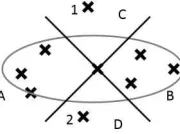
Figure 2.3: Point cloud with ellipse

points. Unlike the finite volume methods which calculate the fluxes at the faces of the control volume, PML calculates the fluxes halfway between the star point of a stencil and all other points in the stencil. The system of equations is linearised, and solved implicitly using approximate, analytical Jacobian matrices where the inviscid flux is obtained from an approximate Riemann solver, and turbulent terms modelled using a one-equation Spalart-Allmaras model. A preconditioned Krylov subspace iterative method is used as the linear solver.

The meshless approach removes the need to generate meshes for complex geometries, and instead only requires simple point distributions of component parts of a model, which PML assembles using the point data to create a large cloud to be used by the solver. The preprocessor to allow this requires a novel stencil selection algorithm which is described in [53]. The stencil selection process makes use of the connectivity in the underlying component meshes to guide the orientation of the ellipses used to select the stencils. For each star point, an ellipse is formed with the semi-major axis as close to perpendicular to the flow direction as possible. The ellipse is divided into quadrants, and a minimum number of points is required in each quadrant to form a stencil. An example is shown in Fig. 2.3, taken from [53].

Increasing the required number of points should increase the stability of the solver, through greater resolution in each stencil. This is however not always possible.

Several cases have been studied including a cylinder undergoing vortex shedding, turbulent aerofoil problems, a three-dimensional fighter aircraft configuration and store release problems with bodies in relative motion. The capability of this solver is par-ticularly useful for modelling control surfaces. This will be demonstrated later in this thesis.

2.2 Control Surface Modelling

(42)

Figure 2.4: NACA 0012 aerofoil point distribution with underlying structural model

that represents the structural elements of a model. In this work, this is a simple beam stick model as shown in Fig. 2.4.

Deformations are prescribed for the structure, which in turn is used to deform the fluid domain. In order to communicate the deformation from the structure to the fluid domain, a mapping is carried out. This mapping describes how much the fluid domain points should be moved for a deformation in the underlying structural grid. At each step within a manoeuvre, the relevant deformation can rapidly be established and applied to the fluid domain points. At the point where the deformed section meets that of the undeformed, the surface is smoothed in a blending procedure. It is also possible, for three-dimensional cases, to insert a cut in the geometry, as would be the case in a physical test. A number of these methods were assessed in [54].

In this work, the deformation technique has been used for the RANS control surface simulations. For the mapping from structure to surface, an interpolation matrix, H is formed, which is used to transfer the displacements between the structural and fluid grids using Eq. (2.8).

(δyf)i= js

X

j=1

hij(δys)j, (2.8)

where (δyf)_i is the displacement of the fluid mesh at node i, (δys)j is the

dis-placement of the structure at node j, and hij are the coefficients of the displacement

(43)

calculated, so that when the structural points are deformed, the fluid point deforms in a manner that maintains the volume of the tetrahedral element. This method is used due to its simplicity and speed of calculation.

The boundary points are moved in line with the interpolation matrix and is de-scribed further in [56]. Once the boundary deformations have been determined, the points in the rest of the computational domain are deformed using an inverse distance approach, as described in [57].

The second approach is to make use of the capabilities of the meshless PML solver. Point distributions are defined for the body and control surface, which are then over-lapped according to the desired deflection. The preprocessor then redefines the bound-aries, removes any points inside the boundary, then reselects the stencils for computa-tion. This has been used for all Euler simulations with a control surface in this work. This approach has the benefit of modelling the control surface in a more realistic man-ner than that of the deformation. There is no smoothing of the edges, as there wouldn’t be on a real aircraft, and the flap is treated as a separate entity to the body.

2.3 Tabular Models

Tabular models are used to determine the flight mechanics loads (the loads subse-quently referred to in this thesis) and moments on manoeuvring aircraft. They are frequently used in the design phase for flight mechanics loads assessment and control systems design. For commercial aircraft the flight envelope can be highly dimensional, with many data points required within the range for each parameter. This can require data points in the order of millions. The data stored in the aerodynamic tables must cover the parameter space in order to effectively simulate manoeuvres. In forming the tables, a number of assumptions are made which give rise to certain limitations. One initial assumption that is made in forming the tables, is that the resolution (i.e. how many data points are in the parameter space) is sufficient to represent the aerody-namic variations of interest. With the tables requiring data to be obtain at millions of points, if CFD is used as the source of the aerodynamic data, it is clearly not feasible to have a solution for each parameter combination. To reduce the number of points required, the parameters can be decoupled. For example, the six dimensional table in Table 2.1, [M,α,β,δele,δail,δrud] can be reduced to four three dimensional tables of

[M,α,β], [M,α,δele], [M,α,δail] and [M,α,δrud]. The assumption here is that the

influ-ence of each decoupled parameter on another is negligible, through the use of small perturbations, which may not be the case for certain flow conditions.

(44)

M α β δele δail δrud CL CD CY Cl Cm Cn

x x x - - - x x x x x x

x x - x - - x x x x x x

x x - - x - x x x x x x

x x - - - x x x x x x x

Table 2.1: Example Aerodynamic Table (x indicates non-zero entry)

proposed in [58], where a 30% reduction in computational time was achieved without loss of accuracy. In [3] this approach was extended to use the DATCOM [59] database as the source of the low-fidelity data, which was then assessed using a commercial jet aircraft case with changing geometry. Kriging interpolation was also applied in this work to further minimise the number of calculations required to fill the tables. It was also used to locate points in the parameter space where a high-fidelity solution is required (i.e. location of high parametric sensitivity).

In this work, only high-fidelity CFD data are used due to the low number of data points required for the cases presented. Kriging is then used to obtain unknown data points within the manoeuvre parameter space.

2.3.1 Dynamic Derivatives

Dynamic derivatives describe how the forces and moments vary with rates of motion. For example, the pitch-damping derivative CMq describes how the pitching moment coefficient,CM, varies with the pitch rate, q. The derivative values are used to account

for motion effects, by taking the static load or moment coefficient and modifying this as shown in Eq. (2.9) for a pitching motion.

Cj(t) =Cj0+Cjα∆α(t) +Cjα˙

c 2U∞

˙

α(t) +Cjq c 2U∞

q(t) +Cjq˙

c 2U∞

2

˙

q(t). (2.9)

The j subscript represents the force or moment of interest (i.e. L,D,M), the zero subscript term is the steady value at timet. The non-dimensionalisation factor is taken from the reduced frequency k = ωc

2U∞. The term ω is in radians per second, as are ˙α and q. This factor maintains consistency with the prescribed inputs, usually k, for describing the oscillatory motion in the calculation of the dynamic derivatives.

For a harmonic pitching motion, the following can be defined

∆α=αAsin(ωt) α˙ =q =ωαAcos(ωt)

¨

(45)

This allows Eq. (2.9) to be rewritten as

Cj(t) =Cj0(t) + ¯Cjαα(t) + ¯Cjqq(t) c 2U∞

, (2.11)

where the bar terms are formed as below again with k= ₂ωc_U ∞.

¯

Cjα = (Cjα−k

2_C

jq˙) ¯

Cjq = (Cjα˙ +Cjq) (2.12)

The derivative values can be calculated from forced periodic oscillations as described in [60]. The periodic time-dependent solution can then be written as a Fourier series, with the first Fourier coefficients corresponding to the values of the stability derivatives. These can be calculated directly using Eq. (2.13),

¯ Cjα =

2 αAncT

Z ncT

0

∆Cj(t) sin(ωt)dt

¯ Cjq =

2 kαAncT

Z ncT

0

∆Cj(t) cos(ωt)dt (2.13)

where the terms αA, k, nc, T and ω are the oscillatory amplitude, reduced frequency,

number of cycles, time period and circular frequency respectively.

Given this model consists of a steady and unsteady component dependent on the instantaneous motion rates, there is no accounting for history effects. As such, this approach is considered as quasi-steady, as described for the CFD solvers previously.

2.4 Frequency Domain Methods

2.4.1 Linear Frequency Domain

The Linear Frequency Domain method [22] uses the assumptions of periodicity and small amplitudes to reduce an unsteady nonlinear problem into a steady linear one.

The governing equations of a fluid are first written in the semi-discrete form as

∂w

∂t +R(w,x,x˙) = 0, (2.14)

where R is the residual, w is the vector of conservative flow variables, with x and ˙x, the grid position and grid velocities respectively.

The assumption of small amplitudes allows the variables to be calculated as a steady state plus a small perturbation about that steady mean state. This gives rise to

w(t) = w¯ + ˜w(t), where w˜

≪

w¯

x(t) = x¯+ ˜x(t), where x˜

≪

x¯

(46)

Combining equations (2.14) and (2.15), leads to the following.

dw˜ dt + ∂R ∂w ¯

w,¯x

˜

w+∂R ∂x ¯

w,x¯

˜

x+∂R ∂x˙

¯

w,x¯

˙˜

x=0 (2.16)

The small periodic time-dependent perturbation is then written as a Fourier series in terms of the base frequencyω and the modek

˜

w(t) =

∞

X

k=1

( ˆwkeikωt), (2.17)

where ˆw is a vector of complex Fourier coefficients corresponding to the flow solu-tion. This is also applied to ˜x. The LFD system can be rewritten by combining equations (2.16) and (2.17) as,

ikωI+ ∂R ∂w

ˆ

wk=−

∂R

∂xˆxk−ikω ∂R

∂x˙ xˆk. (2.18)

Limiting interest to the perturbations which are harmonic in the forced frequency,k is taken to be 1, and hence the nonlinear Eq. (2.14) has been reduced to a single linear equation. The linear system is then solved for ˆwk.

The real and imaginary parts in Eq. (2.18) are taken to form two coupled real systems as

−ω

ℑ

( ˆw) +∂R

∂w

ℜ

( ˆw) = − ∂R

∂x

ℜ

(ˆx) +ω ∂R

∂x˙

ℑ

(ˆx)

ω

ℜ

( ˆw) +∂R

∂w

ℑ

( ˆw) = − ∂R

∂x

ℑ

(ˆx)−ω ∂R

∂x˙

ℜ

(ˆx). (2.19)

The above linear system is written in the form

Ax=b, (2.20)

whereA is the system matrix written as

A=

" ∂R

∂w −ωI

ωI ∂_∂R_w

#

, (2.21)

where x is the vector of Fourier coefficients to be calculated and b is the right-hand side obtained through central finite differences from the steady state solution as

∂R ∂xxˆ ≈

R( ¯w,x¯+ǫˆx,0)−R( ¯w,x¯−ǫxˆ,0) 2ǫ

∂R ∂x˙ xˆ ≈

R( ¯w,x¯, ǫˆx)−R( ¯w,x¯,−ǫxˆ)

2ǫ . (2.22)

(47)

of higher-order terms, but also small enough to reduce the truncation error. Once this linear system has been obtained and set up, it can be solved using a linear solver as described in section 3.1.

2.4.2 Harmonic Balance

The Harmonic Balance method was initially proposed for use in turbomachinery flows for the rapid solution of periodic oscillatory simulations. The benefit is that there is no linearisation involved in the formulation, and as such, nonlinearities can be captured to varying degrees of accuracy depending on the number of harmonics retained in the solution. HB has been extended for use with aircraft aerodynamics and in particular for flight dynamics and the generation of dynamic derivatives.

The formulation again begins with the semi-discrete form of the governing flow equations as

∂w(t)

∂t +R(w) =0, (2.23)

wherewis the vector of conserved variables, andRis the residual of the flux terms. As-suming a periodic motion, these terms can be written as a Fourier series with frequency ω as

w(t) = wˆ0+

∞

X

k=1

( ˆwkeikωt)

R(t) = Rˆ0+

∞

X

k=1

( ˆRkeikωt)). (2.24)

The exponential is broken down into its sine and cosine components, along with the corresponding Fourier coefficients denoted by the subscriptsaandb. The series is then truncated to a specified number of harmonics NH leading to the following

w(t) ≈ wˆ0+

NH

X

k=1

( ˆwakcos(ωkt) + ˆwbksin(ωkt))

R(t) ≈ Rˆ0+

NH

X

k=1

( ˆRakcos(ωkt) + ˆRbksin(ωkt)). (2.25)

Combining Eqs. (2.23) and (2.25), then grouping similar harmonic terms yields

ˆ

R0 = 0

ωnwˆbn+ ˆRan = 0

(48)

A system ofNT = 2NH + 1 equations has now been obtained, which can be written in

matrix form as

ωA ˆw+ ˆR= 0, (2.27)

where A is a block matrix of size NT x NT containing blocks with diagonal terms

A(n+1,NH+n+1) = n, and A(NH+n+1,n+1) = -n. The vectors ˆwand ˆRare composed

of ˆ w=               ˆ w0 ˆ

wa1 .. . ˆ

wa_NH

ˆ

wb1 .. . ˆ

wb_NH               ˆ R=               ˆ R0 ˆ

Ra1 .. . ˆ

Ra_NH

ˆ

Rb1 .. . ˆ

Rb_NH               , (2.28)

where the coefficients are those seen in Eq. (2.25). A solver could be written to solve Eq. (2.27), however this could be complicated due to the complex Fourier terms, par-ticularly when dealing with viscous flows, as well as finding a relationship between ˆw

and ˆR. To overcome this problem, the system is transformed back to the time domain. The solution is discretised intoNT equally spaced intervals over the cycle to obtain

whb=      

w(t0+ ∆t)

w(t0+ 2∆t)

.. .

w(t0+T)

     

Rhb=      

R(t0+ ∆t)

R(t0+ 2∆t)

.. .

R(t0+T)

      , (2.29)

where T is the time for one cycle and ∆t= 2π/(NTω). The vectors in Eq. (2.29) are

initialised from steady state solutions at each of the intervals to provide a good initial guess. The vectors of Fourier terms are then related to the corresponding HB vectors via an NTxNT transformation matrix E

ˆ

(49)

where

E = 2

NT               

0.5 0.5 . . . 0.5

cos(2π1×1

NT ) cos(2π

1×2

NT) . . . cos(2π

1×_N_T

NT )

.. . cos(2πNH×1

NT ) cos(2π

NH×2

NT ) . . . cos(2π

NH×_N_T

NT )

sin(2π1×1

NT) sin(2π

1×2

NT) . . . sin(2π

1×_N_T

NT )

.. . sin(2πNH×1

NT ) sin(2π

NH×2

NT ) . . . sin(2π

NH×_N_T

NT )

               . (2.31)

It is possible to compute one large Fourier transform on the full system, however, in using this matrix with one column per time slice, this has the effect of carrying out lots of small transforms and reduces the computational cost. Substituting Eq. (2.30) into Eq. (2.27) and premultiplying by E−1

gives

ωE−₁

AEwhb+ E

−₁

ERhb= 0. (2.32)

This can then be reduced to

ωDwhb+Rhb= 0, (2.33)

where

D = E−₁

AE = 2 NT

NH

X

k=1

ksin(2πk(j−i)/NT). (2.34)

Equation (2.33) is then solved by introducing a pseudo-time term to be able to time-march the system to achieve a converged solution.

dwhb

dt +ωDwhb+Rhb= 0. (2.35)

Equation (2.35) only differs from Eq. (2.23) by the HB source term ωDwhb. This

allows for simple extension of existing CFD solvers for the solution of this system. The time domain response can be reconstructed from the whb and Rhb vectors through

transformation to the frequency domain, where the Fourier coefficients in Eq. (2.25) are obtained. Solution approaches to equation (2.35) are described in section 3.2.

2.4.2.1 Implicit Solution

(50)

time slices. This is defined as follows        ∂R ∂w _t

0+∆t ωD1,2 . . . ωD1,NT

ωD2,1 ∂_∂R_w

t0+2∆t ..

. . ..

ωDNT,1 ωDNT,2

∂R

∂w

_t

0+T

       (2.36)

The diagonal terms are the Jacobian matrices of the individual time slices, and the off–diagonal terms are taken from the HB source term in Eq. (2.35). This approach allows rapid solution of the Harmonic Balance problem with linear solvers and are used in this thesis with the PML solver.

2.4.3 ILU Preconditioner

The linear system in Eq. (2.20) ideally would be solved by finding the inverse of A and then multiplying this by the right hand side to obtain x. However, finding the inverse of the very large sparse matrices encountered in CFD using direct methods is computationally expensive. The alternative used is to take the linear system and represent it as an equivalent system, which is better conditioned, and thus quicker to iteratively solve. This is done with the use of a preconditioning matrix P which is an approximation ofA, and can be inverted easily. This is used as shown in Eq. (2.37) for left preconditioning:

P−1

Ax=P−1

b (2.37)

and in Eq. (2.38) for right preconditioning

AP−1

Px = AP−1 y=b

wherex = P−1

y. (2.38)

If P−1

is equal to the inverse of A, an identity matrix is obtained on the left hand side and the system is solved. The most simple preconditioning technique is Jacobi

Preconditioning, where the preconditioner matrix is a diagonal matrix with the inverse

of the diagonal terms of Aalong it.

(51)

non-zeros have been added. In this work up to 1 level of fill-in is used, which usually adds around two further non-zeros for every one in the A matrix, although this varies slightly depending on the problem. The algorithm for the ILU factorisation is as follows

1. For all non-zero elements aij define lev(aij) = 0

2. Fori= 2, . . . , n Do:

3. Fork= 1, . . . , i−1 and for lev(aik)≤p Do:

4. Computeaik =aik/akk

5. Computeai∗=ai∗−aikak∗

(where * indicates operation on all non-zero terms in the row) 6. Update the levels of fill of the non-zeroaij’s using:

levij =min{levij, levik+levkj + 1}

7. EndDo

8. Replace any element in row iwithlev(aij)> pby zero

9. EndDo

(52)

(53)

Chapter 3

Performance of Frequency

Domain Methods

Frequency domain methods have proven useful for flight dynamics purposes. They offer accelerated computation of the aerodynamic response to a periodic oscillation required to calculate the dynamic derivative terms in the unsteady aerodynamic model. This chapter looks to accelerate the Linear Frequency Domain and Harmonic Balance methods, through an approach to preconditioning for linear solvers.

3.1 Linear Frequency Domain

The origins of the Linear Frequency Domain method are in the small disturbance Euler method developed for use in turbomachinery flows by Hall and Crawley [24]. It has since been extended for use in external aerodynamic problems. It has been implemented in the DLR TAU code, as described in [22], and forms the basis of the method described in this chapter.

3.1.1 Solver Options

There are a number of different solution methods available for solving the linear systems in the LFD formulation. In order to improve upon them, it is first necessary to assess how well they perform in their current form. Three approaches are available within TAU, namely MG LU-SGS, PETSc and a Generalised Conjugate Residual (GCR) linear solver, the latter of which has been implemented as part of this work.

MG LU-SGS

The MG LU-SGS option is implemented within TAU and drives the solution to con-vergence by solving

˜

(54)

where ˜A is an approximation of A, and the matrix-vector product ˜Axis driven to an L2 norm of zero. This is done using the semi-implicit LU-SGS iterative solver [36] with Multigrid [51] to accelerate the convergence. The MG LU-SGS option can also be used with a GMRes [61] Krylov solver, in order to further accelerate the convergence, but at the expense of memory. This method only operates on the matrix-vector product and never stores the full Jacobian matrix explicitly in memory. This minimises the memory requirement to enable very large grids to be run on relatively inexpensive machines, and gives this approach a competitive edge over the other two solver options, in this sense.

PETSc Linear Solvers

The second option is to use the linear solvers built into the PETSc linear libraries [62, 63]. TAU can be compiled with the PETSc libraries for solution of both the Adjoint and LFD problems. The implementation requires the storage of the Jacobian matrix explicitly in memory, and as such requires significantly more memory than MG LU-SGS. The PETSc libraries include many solvers, from the direct LU and Cholesky methods through to the approximate Krylov methods, including GCR and GMRes used in this work. PETSc also has a variety of preconditioners, ranging from the simple Jacobi preconditioning to the ILU factorisation used here. The solvers also have many options to monitor convergence properties, along with other options to improve convergence such as Reverse Cuthill-McKee reordering. This array of solver options makes PETSc a useful tool for optimising the linear solution.

Generalised Conjugate Residual Linear Solver

The final option is the GCR [64] linear solver. This method has been implemented in TAU for solution of the LFD problem as part of this work. It uses a block matrix structure rather than an element-wise structure to minimise the memory required to store the sparse matrix, and to increase the speed with which the data can be accessed. This requires a blocked version of the ILU(k) preconditioner mentioned in Section 2.4.3. As with PETSc, the full Jacobian matrix is stored in memory.

The GCR solver is a Krylov subspace method whereby the system is projected onto a subspace shown in Eq. (3.2).

Km(A,r0) =span{r0, Ar0, A2r0, ..., Am−1r0}, (3.2)

wheremis the number of subspace vectors allocated in advance, and the residual r0 is