This is a repository copy of
An efficient nonlinear cardinal B-spline model for high tide
forecasts at the Venice Lagoon
.
White Rose Research Online URL for this paper:
http://eprints.whiterose.ac.uk/1945/
Article:
Wei, H.L. and Billings, S.A. (2006) An efficient nonlinear cardinal B-spline model for high
tide forecasts at the Venice Lagoon. Nonlinear Processes in Geophysics, 13 (5). pp.
577-584. ISSN 1607-7946
[email protected] https://eprints.whiterose.ac.uk/ Reuse
Unless indicated otherwise, fulltext items are protected by copyright with all rights reserved. The copyright exception in section 29 of the Copyright, Designs and Patents Act 1988 allows the making of a single copy solely for the purpose of non-commercial research or private study within the limits of fair dealing. The publisher or other rights-holder may allow further reproduction and re-use of this version - refer to the White Rose Research Online record for this item. Where records identify the publisher as the copyright holder, users can verify any specific terms of use on the publisher’s website.
Takedown
If you consider content in White Rose Research Online to be in breach of UK law, please notify us by
www.nonlin-processes-geophys.net/13/577/2006/ © Author(s) 2006. This work is licensed
under a Creative Commons License.
Nonlinear Processes
in Geophysics
An efficient nonlinear cardinal B-spline model for high tide forecasts
at the Venice Lagoon
H. L. Wei and S. A. Billings
Department of Automatic Control and Systems Engineering, University of Sheffield, Mappin Street, Sheffield, S1 3JD, UK
Received: 19 July 2006 – Revised: 16 October 2006 – Accepted: 16 October 2006 – Published: 23 October 2006
Abstract. An efficient class of nonlinear models, con-structed using cardinal B-spline (CBS) basis functions, are proposed for high tide forecasts at the Venice lagoon. Ac-curate short term predictions of high tides in the lagoon can easily be calculated using the proposed CBS models.
1 Introduction
The Venice lagoon is one of the world’s most delicate and unstable ecosystems. Since the disastrous flood that occurred in November 1966, the problems of the Venice lagoon have become one of national and international interest. The threat-ened Venice city has frequently been inundated by high wa-ters formed in the northern Adriatic Sea, where interactions of several astronomical and meteorological phenomena often occur. The end results are the Venice floods due to a combi-nation of astronomical and meteorological effects: the tides induced by the moon and the tides caused by stormy weather arise from low atomospheric pressure combined with winds. To prevent disastrous floods, measures have been taken since 1966, and perhaps the most famous project is the recently endorsed MoSE (Modulo Sperimentale Elettromeccanico— Experimental Electromechanical Module) project, although the feasibility of this project is still in public debate (Rosen-thal, 2005; Salzano, 2005). A parallel and complementary approach to engineering constructions, for example the bar-rier system as involved in the MoSE, is to build an opera-tional flood warning system, which is used to forecast the main surge, for some time ahead ideally many hours or even several days. The objective of such a flood warning system is to support some necessary actions such as the removal of goods from ground floors, the redirection of the city boat traffic, and the installation of elevated pedestrian walkways
Correspondence to: H. L. Wei
(Vieira et al., 1993). The flood warning system is model-based: it utilises both statistical and hydrodynamic models to obtain short term as well as long term forecasts (Vieira et al., 1993). The hydrodynamic modelling usually starts with first principles that require a comprehensive physical insight into the underlying dynamics of the system, whereas the sta-tistical modelling and similar methods often start with ob-servational data, based on which mathematical models that support forecasts of the main surge are deduced.
Several authors have discussed the data-based modelling problem relating to high tide forecasts at the lagoon, by treat-ing the regularly measured water level as a nonlinear time series, with the assumption that no information on the hydro-dynamics of the lagoon is involved, but merely observed wa-ter level data are available (Zaldivar et al., 2000). Many ap-proaches have been proposed to model the associated nonlin-ear time series including nonlinnonlin-ear regression models, chaos and embedding methods, neural networks, evolutionary al-gorithms, and other methods, see Zaldivar et al. (2000) and del Arco-Calderon et al. (2004) and the references therein.
578 H. L. Wei and S. A. Billings: Cardinal B-spline model for high tide forecasts
Table 1. Cardinal B-splines of order 1 to 4.
N1(x) N2(x) 2N3(x) 6N4(x)
0≤x<1 1 x x2 x3
1≤x<2 0 2−x −2x2+6x−3 −3x3+12x2−12x+4 2≤x<3 0 0 (x−3)2 3x3−24x2+60x−44 3≤x≤4 0 0 0 −x3+12x2−48x+64
elsewhere 0 0 0 0
provide not only accurate short term forecasts, but also pro-vide good long term predictions for the variation of water levels in the lagoon. Compared with existing data-based methods, the proposed data-based CBS modelling approach can produce more accurate predictions for high tides at the Venice lagoon.
2 Time series forecasting problem
Let{y(t )}T
t=t0 be a known observed sequence for the
under-lying dynamical time series. The goal of multi-step-ahead forecasts is to predict the values ofy(t+s), withs≥1, using the information carried by the observed sequence{y(t )}T
t=t0.
To achieve such a goal, a commonly used approach is to learn a model, or a predictor, from the available data. To obtain multi-step-ahead predictions of nonlinear time series, both iterative and direct methods can be employed (Wei and Billings, 2006). In theory, long-term predictions can be ob-tained from a short-term predictor, for example a one-step-ahead predictor, simply by applying the short predictor many times in an iterative way. This is called iterative prediction. Direct prediction, however, provides a once-completed pre-dictor and multistep forecasts can be obtained directly from the established predictor in a way that is similar to computing one step predictions.
Following Wei and Billings (2006), a direct approach will be considered. Take the case of thes-step-ahead forecasting problem as an example. The task fors-step-ahead forecasts is to find a model that can predict the value ofy(t+s)using a set of selected variables{y(t ),y(t−1),· · ·, y(t−d+1)}, in the sense that
y(t+s)=f(s)(y(t ),· · ·, y(t−d+1))+e(t ) (1)
wheref(s)withs≥1 are some nonlinear functions,e(t )is an unpredictable zero mean noise sequence,dis the model order (the maximum lag). For a real system, the nonlinear function f(s) is generally unknown and might be very complex. A class of models that are both flexible, with excellent approx-imation capabilities, and which can represent a broad class of highly complex systems are therefore required to ensure accurate directs-step predictions. The model class that uses cardinal B-splines as the basis functions to approximate the
s-step predictorf(s)(·)satisfies all these conditions and will
therefore be investigated in the present study as a new ap-proach of achieving accurate directs-step predictions.
3 Cardinal B-spline models
3.1 Cardinal B-splines
Themth order cardinal B-spline function is defined by the following recursive formula (Chui, 1992):
Nm(x)= x
m−1Nm−1(x)+ m−x
m−1Nm−1(x−1), m≥2 (2)
where
N1(x)=χ[0,1)(x)=
1 ifx ∈ [0,1)
0 otherwise (3)
It can easily be shown that the support of the mth order B-spline function is suppNm=[0, m]. Compared with other
basis functions, the most attractive and distinctive prop-erty of B-splines are that they are compactly supported and can be analytically formulated in an explicit form. Most importantly, they form a multiresloution analysis (MRA) (Chui, 1992). B-splines are unique, among many com-monly used basis functions, because they simultaneously possess the three remarkable properties, namely compactly supported, analytically formulated and multiresolution anal-ysis oriented, among many popular basis functions. These splendid properties make B-splines remarkably appropriate for nonlinear dynamical system modelling. The most com-monly used B-splines are those of orders 1 to 4, which are shown in Table 1.
For the mth order B-spline function Nm∈L2(R), let Nj,km(x)=2j/2Nm(2jx−k),Djm={Nj,km :k∈Z}, wherej, k∈Z
are called the scale (or dilation) and position (translation) parameters respectively. Following (Chui, 1992), for each j∈Z, let Vjm denote the closure of the linear span of Djm, namely, Vjm=closL2(R)<Djm>. The following properties
(Chui, 1992) possessed byDmj andVjmform the foundations of the cardinal B-spline multiresolution analysis modelling framework for nonlinear dynamical systems:
i) For any pair of integersmandj, withm≥2, the family Dmj={Nm
j,k(x):k∈Z}is a Riesz basis ofVjmwith Riesz
boundA=Am(Amis a constant related tom) andB=1.
Furthermore, these bounds are optimal.
ii) Themth order B-spline functionNmis a scaling function
andVjmforms a multiresolution analysis (MRA).
From the above discussions, for every function f∈Vm j ,
there exists a unique sequence{cm
k}k∈Z∈ℓ2(Z)such that
f (x)=X k∈Z
ckm2j/2Nm(2jx−k) (4)
For convenience of description, the symbolφwill be intro-duced to represent themth order B-spline functionNm and
the symbol “m” will be omitted in associated formulas.
3.2 The cardinal B-spline model for high dimensional problems
The result for the 1-D case described above can be extended to high dimensions and several approaches have been pro-posed for such an extension. Tensor product and radial con-struction are two commonly used methods (Wei and Billings, 2004; Billings and Wei, 2005). Following the idea in Hastie and Tibshirani (1990) and Kavli (1993), in the present study, a linear additive CBS model structure will be employed to represent a high dimensional nonlinear function. Kavli (1993) suggested a method to successively refine a linear B-spline model for multivariate problems by adding new 1-D submodels step by step.
For ad-dimensional functionf∈L2(Rd), the linear
addi-tive representation is given below
f (x1, x2,· · ·, xd)=f1(x1)+f2(x2)+ · · · +fd(xd) (5)
where fr∈L2(R) (r=1,2,. . . ,d) are univariate functions,
which can be expressed using the expansion (4) as below
fr(xr)=
X
k∈Z
crj,kφj,k(xr) (6)
whereφj,k(x)=2j/2φ (2jx−k), andj, k∈Zare the scale and
position parameters, respectively.
Now consider the model given by Eq. (1) and let xr(t )=y(t−r+1)forr=1, 2,. . . , d. Using Eqs. (5) and (6),
model (1) can be expressed as
y(t+s)= d X
r=1
fr(s)(xr(t ))= d X
r=1
X
k∈Z
c(s,r)j,k φj,k(xr(t ))+e(t ) (7)
The remaining task is how to deduce, from Eq. (7), a parsi-monious model that can be used fors-step-ahead forecasts for a given prediction horizon s. The following problem needs to be solved:
– How to choose the scale and position parametersj and k?
– In practical modelling problems, the variables xr(t )
(r=1, 2, . . . , d), as the lagged versions of y(t ), are usually sparsely distributed in the associated space and therefore the problem may be ill-posed. The representa-tion (7) is thus often redundant in the sense that most of the basis functions (or model terms),φj,k(·)in Eq. (7),
can be removed from the model, and experience shows that only a small number of significant model terms are required for most nonlinear dynamical modelling prob-lems. The question is: how to select the potential sig-nificant model terms from a large number of candidate basis functions?
The scale and position determination problem will be dis-cussed in the following section. The model term selection problem has been systematically investigated in Billings et al., 1989; Chen et al., 1989). In the present study, an orthog-onal least squares (OLS) algorithm, interfered with by an er-ror reduction ratio (ERR) index (Billings et al., 1989; Chen et al., 1989), and regularized by a Bayesian information crite-rion (BIC) (Schwarz, 1978; Efron and Tibshirani, 1993), will be used to select significant model terms and to determine the model size (the number of model terms included in the final model). One version of the OLS-ERR type algorithm, called the forward orthogonal regression (FOR) algorithm, is pre-sented in the Appendix.
3.3 Determination of the scale and position parameters
Assume that ad-variate functionf of interest is defined in the unit hypercube[0,1]d. Consider the scale parameter de-termination problem first. Experience on numerous simula-tion studies relating to wavelet multiresolusimula-tion modelling for dynamical nonlinear systems, for example Wei et al. (2004a, b) and Wei and Billings (2004) and the references therein, has shown that the scale parameterj in model (7) should not be chosen too large. A value that is between zero and two or three forj is often adequate for most nonlinear dynamical modelling problems.
For cardinal B-spline functions, the position parameterk is dependent on the corresponding resolution scalej. Indeed, for each fixed pointx∈[0,1], sinceNmhas compact support,
all except a finite number of terms in the expression (4) are zero. Take the 4th-order B-spline function as an example. At a given scalej, the non-zero terms are determined by the po-sition parameterkfork=−3,−2,−1,· · ·,2j−1. In general, for the B-spline function of orderm, whose support is[0, m], the support for the associated functionφj,k(x)=2j/2(2jx−k)
is[2−jk,2−j(m+k)], therefore, the position parameterk at a resolution scalejshould be chosen as−(m−1)≤k≤2j−1.
4 Water level modelling and high tide forecasting
4.1 The data
580 H. L. Wei and S. A. Billings: Cardinal B-spline model for high tide forecasts
0 50 100 150 200
-40 -20 0 20 40 60 80 100 120 140
Time [hr]
W
a
te
r
L
e
v
e
l
[c
m
[image:5.595.51.280.64.244.2]]
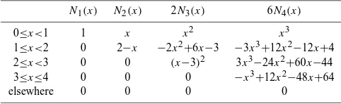
Fig. 1. One-hour-ahead prediction for typical high tides. The thin
line with dots indicates the measurements (observed in 1993), and the thick dashed line indicates the prediction values.
water levels in 1993 and the predicted values will then be compared with the real observations.
The maximum lag for the input variables in the initial modelling procedure was chosen to be 24, to cover the range of the maximum oscillation cycle of the related time series. Thus, the variablesy(t ), y(t−1),· · ·, y(t−23)were used as inputs to form a predictor, whose output was the future be-haviour, denoted byy(t+s)(s≥1).
Note that the original data were initially normalized to [0,1] via a transformy(t )=(y(t )−a)/(b−a)˜ , wherey(t )˜ in-dicate the initial observations, anda=−100 andb=150. The identification procedure was therefore performed using nor-malized valuesy(t ). The outputs of an identified model were then recovered to the original measurement space by taking the associated inverse transform.
4.2 The models
Letxr(t )=y(t−r+1),r=1, 2,. . . , 24. The structure of the
initial CBS model was chosen to be
y(t+s)= 24
X
r=1 0
X
k=−3
c(s,r)0,k φ0,k(xr(t ))
+ 24
X
r=1 1
X
k=−3
α(s,r)1,k φ1,k(xr(t )) (8)
where φj,k(x)=2j/2φ (2jx−k),with j, k∈Z, are the
4th-order B-spline functions. Notice that model (8), which in-volves two scale levels forj=0 andj=1, is in structure dif-ferent from model (7), where the model termφj,k(·)only
in-volves a single scale level. The reason that the initial model (8) was chosen to be such a structure was to enrich the pool of the model term dictionary, so that basis functions with dif-ferent scale parameters can be sufficiently utilised. Although
0 50 100 150 200
-40 -20 0 20 40 60 80 100 120 140
Time [hr]
W
a
te
r
L
e
v
e
l
[c
m
[image:5.595.310.543.64.244.2]]
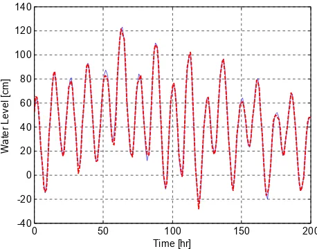
Fig. 2. Four-hour-ahead prediction for typical high tides. The thin
solid line indicates the measurements (observed in 1993), and the thick dashed line indicates the prediction values.
a total number of 216 model terms (basis functions) were in-volved in the initial model (8) for any givens, only a small number of basis functions were required to describe the re-lationship between{y(t ), y(t−1),· · ·, y(t−23)}andy(t+s), and significant model terms were efficiently selected by per-forming a model term detection algorithm,. Also, different values fors usually led to different final models. For each s, an OLS-ERR algorithm (Billings et al., 1989; Chen et al., 1989), regularized by a Bayesian information criterion (BIC) (Schwarz, 1978; Efron and Tibshirani, 1993), was used to determine the number of model terms, and the parameters of the final CBS model was then re-estimated by introducing a linear moving average (MA) model of order 10 (Billings and Wei, 2005; Wei and Billings, 2006).
4.3 Prediction results
Eight cases, corresponding to s=1, 4, 12, 24, 28, 48, 72, and 96, were considered, and eight different CBS models were identified for each of four data sets “data90”, “data91”, “data92”, and “data93”. The resultant eight models were ap-plied respectively over four test data sets, “data91”, “data92”, “data93”, and “data94”, to calculates-step-ahead forecasts of water levels. Prediction performance, measured by the root-mean-square-errors (RMSE) as used in Zaldivar et al. (2000) and del Arco-Calderon et al. (2004), over the four test data sets, obtained from the identified CBS models, are shown in Table 2. Compared with the results produced by multilayer neural networks (Zaldivar et al., 2000) and evolutionary algo-rithms (del Arco-Calderon et al., 2004), the results produced by the proposed CBS models are better, both for short and long term predictions.
To visually illustrate the performance of the identified CBS models for high tide forecasting, both short term and
Table 2. Prediction errors for water levels of the years 1991, 1992, 1993, and 1994, with 8760, 8784, 8760, and 8760 records, respectively.
Prediction horizon 1991 1992 1993 1994
Model size RMSE Model size RMSE Model size RMSE Model size RMSE
1 39 1.521 38 1.538 49 1.519 37 1.489
4 36 5.389 35 5.408 35 5.274 31 5.075
12 24 7.072 21 7.406 18 6.656 20 6.439
24 23 7.325 16 7.353 18 6.858 19 6.584
28 27 9.232 26 9.246 26 8.637 23 8.352
48 22 10.686 18 10.752 23 9.788 20 9.716
72 20 13.036 21 13.352 23 12.019 19 11.940
96 18 14.480 23 15.108 25 13.576 21 13.449
0 50 100 150 200
-40 -20 0 20 40 60 80 100 120 140
Time [hr]
W
a
te
r
L
e
v
e
l
[c
m
[image:6.595.53.284.246.423.2]]
Fig. 3. Twelve-hour-ahead prediction for typical high tides. The
thin solid line indicates the measurements (observed in 1993), and the thick dashed line indicates the prediction values.
long term predictions for some high tides were calculated using the identified CBS models. Taking the prediction re-sults for some typical high tides in the year 1993 as an exam-ple, the 1-, 4-, 12-, and 24-h-ahead predictions are shown in Figs. 1 to 4, respectively.
It can be seen from Figs. 1 to 4 that albeit the identified CBS models can produce very good short term (4 h-ahead) predictions for typical high tides at the lagoon, the resul-tant models can not effectively produce long (>12 h-ahead) term predictions for high waters (water level>110 cm). The reason that the models can not provide effective long term predictions may be that the “input” signals, considered here, for the associated dynamical models may not be sufficient to describe the real world dynamical systems, in other words, additional input signals may be required to adequately char-acterize the underlying dynamical behaviour. One solution to this problem is likely to involve multiple time series, and tides at several places in the Adratic Sea or the use of a 3-D
0 50 100 150 200
-40 -20 0 20 40 60 80 100 120 140
Time [hr]
W
a
te
r
L
e
v
e
l
[c
m
]
Fig. 4. Twenty-four-hour-ahead prediction for typical normal water
level. The thin solid line indicates the measurements (observed in 1993), and the thick dashed line indicates the prediction values.
hydrodynamical model with adequate forcing. Following the idea of Cao et al. (1998), the extension of the methodology to multiple time series approach, will be addressed in a future paper.
5 Conclusions
[image:6.595.310.542.246.427.2]582 H. L. Wei and S. A. Billings: Cardinal B-spline model for high tide forecasts
Appendix A The forward orthogonal regression algorithm
The CBS models are based on a prescribed prototype func-tion, and temporal analysis is performed using some dilated and translated versions of the same function. Data analy-sis can thus be implemented using the corresponding coef-ficients. The initial CBS model (8), where each basis func-tion (model regressor) is a variant of the same cardinal B-spline function, can easily be converted into a linear-in-the-parameters form
y(t )= M
X
m=1
θmψm(t )+e(t ) (A1)
where x(t )=[x1(t ), x2(t ),· · ·, xd(t )]T, with xr(t )=y(t−r+1) for r=1,2,. . . ,d, is the “input”
(pre-dictor) vector, ψm(t )=ψm(x(t )) are the model regressors, θmare the model parameters, andM is the total number of
candidate regressors.
The initial regression model (A1) often involves a large number of candidate model terms. Experience suggests that most of the candidate model terms can be removed from the model, and that only a small number of significant model terms are needed to provide a satisfactory representation for most nonlinear dynamical systems. The orthogonal least square (OLS) type algorithms (Billings et al., 1989; Chen et al., 1989) interfered with by an error reduction ratio (ERR) index, can be used to select significant model terms, and a Bayesian information criterion (BIC) (Schwarz, 1978; Efron and Tibshirani, 1993), can be used to aid the determination of the associated model size (Wei et al., 2006).
Consider the term selection problem for the linear-in-the-parameters model (A1). Let {(x(t ), y(t )):x∈Rd, y∈R}Nt=1 be a given training data set andy=[y(1),· · ·, y(N )]T be the
vector of the output. LetI = {1,2,· · ·, M}, and denote by ={ψm:m∈I}the dictionary of candidate model terms in an
initially chosen candidate regression model similar to (A1). The dictionarycan be used to form a variant vector dic-tionaryD={φm:m∈I}, where themth candidate basis vector φm is formed by the mth candidate model termψm∈, in
the sense thatφm=[ψm(x(1)),· · ·, ψm(x(N ))]T. The model
term selection problem is equivalent to finding, fromI, a sub-set of indices,In={im:m=1,2,· · ·, n, im∈I}wheren≤M, so
that y can be approximated using a linear combination of αi1,αi2,· · ·,αin.
A1 The forward orthogonal regression procedure
A non-centralised squared correlation coefficient will be used to measure the dependency between two associated ran-dom vectors. The non-centralised squared correlation coeffi-cient between two vectorsxandyof sizeNis defined as
C(x,y)= (x Ty)2
||x||2||y||2 =
(xTy)2 (xTx)(yTy) =
(PN
i=1xiyi)2
PN
i=1x2i
PN
i=1yi2
(A2)
The squared correlation coefficient is closely related to the error reduction ratio (ERR) criterion (a very useful index in respect to the significance of model terms), defined in the standard orthogonal least squares (OLS) algorithm for model structure selection (Billings et al., 1989; Chen et al., 1989).
The model structure selection procedure starts from Eq. (A1). Letr0=y, and
ℓ1=arg max
1≤j≤M{C(
y,φj)} (A3)
where the functionC(·,·)is the correlation coefficient de-fined by (A2). The first significant basis can thus be selected asα1=φℓ1, and the first associated orthogonal basis can be
chosen asq1=φℓ1. The model residual, related to the first
step search, is given as
r1=r0− yTq1
qT1q1
q1 (A4)
In general, themth significant model term can be chosen as follows. Assume that at the (m-1)th step, a subset Dm−1,
consisting of (m−1) significant bases, α1,α2,· · ·,αm−1,
has been determined, and the (m−1) selected bases have been transformed into a new group of orthogonal bases q1,q2,· · ·,qm−1via some orthogonal transformation. Let
q(m)j =φj− m−1
X
k=1 φTjqk
qTkqk
qk (A5)
ℓm=arg max
j6=ℓk,1≤k≤m−1
{C(y,q(m)j )} (A6)
where φj∈D−Dm−1, and rm−1 is the residual vector
ob-tained in the (m−1)th step. Themth significant basis can then be chosen asαm=φℓm and themth associated
orthogo-nal basis can be chosen asqm=q(m)ℓm. The residual vectorrm
at themth step is given by
rm=rm−1− yTqm qT
mqm
qm (A7)
Subsequent significant bases can be selected in the same way step by step. From (A7), the vectorsrmandqmare
orthogo-nal, thus
||rm||2= ||rm−1||2−
(yTqm)2 qT
mqm
(A8)
By respectively summing (A7) and (A8) formfrom 1 ton, yields
y= n
X
m=1 yTqm qT
mqm
qm+rn (A9)
||rn||2= ||y||2− n
X
m=1
(yTqm)2 qT
mqm
(A10)
The model residualrn will be used to form a criterion for
model selection, and the search procedure will be terminated when the norm ||rn||2 satisfies some specified conditions.
Note that the quantityERRm=C(y,qm)is just equal to the mth error reduction ratio (Billings et al., 1989; Chen et al., 1989), brought by including themth basis vectorαm=φℓm
into the model, and thatPn
m=1C(y,qm)is the increment or
total percentage that the desired output variance can be ex-plained byα1,α2,· · ·,αn.
In the present study, the following Bayesian information criterion (BIC) (Schwarz, 1978; Efron and Tibshirani, 1993) is used to determine the model size
BIC(n)=N+n[ln(N )−1]
N−n MSE(n) (A11)
In the present study, the mean-squared-error (MSE) in (A11) is defined as
MSE(n)=||rn||
2
2N = 1 2N
XN
t=1[y(t )− ˆy(t )]
2 (A12)
where y(t )ˆ is the model prediction produced from the as-sociated model ofnterms. The model size will be chosen as the value where the index function BIC(n)is minimized. Note that other popular definitions for MSE in (A11) are also available, for example, MSE(n)=||rn||2/N(Wei et al. 2006).
A2 Parameter estimation
It is easy to verify that the relationship between the selected original basesα1,α2,· · ·,αn, and the associated orthogonal
basesq1,q2,· · ·,qn, is given by
An=QnRn (A13)
whereAn=[α1,· · ·,αn],Qnis anN×nmatrix with
orthog-onal columns q1,q2,· · ·,qn, and Rn is an n×n unit
up-per triangular matrix whose entriesuij(1≤i≤j≤n)are
cal-culated during the orthogonalization procedure. The un-known parameter vector, denoted byθn=[θ1, θ2,· · ·, θn]T,
for the model with respect to the original bases, can be calculated from the triangular equation Rnθn=gn
withgn=[g1, g2,· · ·, gn]T , wheregk=(yTqk)/(qTkqk)for k=1,2, . . . ,n.
Acknowledgements. The authors gratefully acknowledge that this work was supported by EPSRC (UK). They are grateful to J. M. Zaldivar Comenges and C. L. del Arco-Calder´on for the constructive comments and helpful suggestions for improving the manuscript.
Edited by: R. Grimshaw
Reviewed by: C. L. del Arco-Calder´on and J. M. Zaldivar Comenges
References
Billings, S. A., Chen, S., and Korenberg, M. J.: Identification of MIMO non-linear systems suing a forward regression orthogonal estimator, Int. J. Control, 49(6), 2157–2189, 1989.
Billings, S. A. and Wei, H. L.: A new class of wavelet networks for nonlinear system identification, IEEE Trans. Neural Networks, 16(4), 862–874, 2005.
Cao, L. Y., Mees, A., and Judd, K.: Dynamics from multivariate time series, Physica D, 121, 75–88, 1998.
Chandre, C., Wiggins, S., and Uzer, T.: Time-frequency analysis of chaotic systems, Physica D, 181, 171–196, 2003.
Chen, S., Billings, S. A., and Luo, W.: Orthogonal least squares methods and their application to non-linear system identification, Int. J. Control, 50(5), 1873–1896, 1989.
Chui, C. K.: An Introduction to Wavelets, Academic Press, Boston, 1992.
del Arco-Calderon, C. L., Vinuela, P. I., and Castro, J. C. H.: Fore-casting time series by means of evolutionary algorithms, Lecture Notes in Computer Science, 3242, 1061–1070, 2004.
Efron, B. and Tibshirani, R. J.: An Introduction to the Bootstrap, Chapman & Hall, New York, 1993.
Grinsted, A., Moore, J. C., and Jevrejeva, S. : Application of the cross wavelet transform and wavelet coherence to geophysical time series, Nonlin. Processes Geophys., 11, 561–566, 2004. Hastie, T. J. and Tibshirani, R. J. : Generalized additive models,
London, Chapman & Hall, 1990.
Kallache, M., Rust, H. W., and Kropp, J.: Trend assessment: ap-plications for hydrology and climate research, Nonlin. Processes Geophys., 12, 201–210, 2005.
Kavli, T.: ASMOD – an algorithm for adaptive spline modeling of observation data, Int. J. Control, 58(4), 947–967, 1993. Kumar, P. and Foufoula-Georgiou, E.: Wavelet analysis for
geo-physical applications, Rev. Geophys., 35(4), 385–412, 1997. Malamud, B. D. and Turcotte, D. L.: Self-affine time series I:
gen-eration and analyses, Adv. Geophys., 40, 1–90, 1999a.
Malamud, B. D. and Turcotte, D. L.: Self-affine time series: mea-sures of weak and strong persistence, J. Stat. Plan. Infe., 80, 173– 196, 1999b.
Maraun, D. and Kurths, J.: Cross wavelet analysis: significance testing and pitfalls, Nonlin. Processes Geophys., 11, 505–514, 2004.
Rosenthal, E.: Venice turns to future to rescue its past, The New York Times Electronic Edition, online: http://www.nytimes.com/ 2005/02/22/science/22veni.html, 22 February 2005.
Salzano, E.: The Venice Lagoon: what it is, what they are doing on it, Eddyburg, online: http://www.eddyburg.it/article/articleview/ 1355/1/122, August 2005.
Schwarz, G.: Estimating the dimension of a model, Ann. Stat., 6(2), 461–464, 1978.
Vieira, J., Fons, J., and Cecconi, G.: Statistical and hydrodynamic models for the operational forecasting of floods in the Venice Lagoon, Coastal Engineering, 21(4), 301–331, 1993.
Wei, H. L., Billings, S. A., and Balikhin, M.: Analysis of the geo-magnetic activity of the D-st index and self-affine fractals using wavelet transforms, Nonlin. Processes Geophys., 11, 303–312, 2004a.
584 H. L. Wei and S. A. Billings: Cardinal B-spline model for high tide forecasts
Wei, H. L. and Billings, S. A.: Identification and reconstruction of chaotic systems using multiresolution wavelet decompositions, Int. J. Syst. Sci., 35(9), 511–526, 2004.
Wei, H. L. and Billings, S. A.: Long term prediction of nonlinear time series using multiresolution wavelet models, Int. J. Control, 79(6), 569–580, 2006.
Wei, H. L., Billings, S. A., and Balikhin, M. A. :Wavelet based nonparametric NARX models for nonlinear input-output system identification, Int. J. Syst. Sci., accepted, to appear in 37(15), 2006.
Zaldivar, J. M., Guti´errez, E., Galv´an, I. M., Strozzi, F., and Tomasin, A.: Forecasting high waters at Venice Lagoon using chaotic time series analysis and nonlinear neural networks, J. Hy-droinformatics, 2(1), 61–84, 2000.