The identification of cellular automata

This is a repository copy of The identification of cellular automata_. White Rose Research Online URL for this paper:

http://eprints.whiterose.ac.uk/74597/

Monograph:

Zhao, Y. and Billings, S.A. (2006) The identification of cellular automata. Research Report. ACSE Research Report no. 938 . Automatic Control and Systems Engineering, University of Sheffield

eprints@whiterose.ac.uk https://eprints.whiterose.ac.uk/ Reuse

Unless indicated otherwise, fulltext items are protected by copyright with all rights reserved. The copyright exception in section 29 of the Copyright, Designs and Patents Act 1988 allows the making of a single copy solely for the purpose of non-commercial research or private study within the limits of fair dealing. The publisher or other rights-holder may allow further reproduction and re-use of this version - refer to the White Rose Research Online record for this item. Where records identify the publisher as the copyright holder, users can verify any specific terms of use on the publisher’s website.

Takedown

If you consider content in White Rose Research Online to be in breach of UK law, please notify us by

The Identification of Cellular Automata

Y. Zhao, S.A. Billings

Research Report No. 938

Department of Automatic Control and Systems Engineering The University of Sheffield

Mappin Street, Sheffield, S1 3JD, UK

The Identification of Cellular Automata

Zhao, Y., Billings, S.A.

September 4, 2006

Abstract

Although cellular automata have been widely studied as a class of the spatio

temporal systems, very few investigators have studied how to identify the CA rules

given observations of the patterns. A solution using a polynomial realization to

describe the CA rule is reviewed in the present study based on the application of an

orthogonal least squares algorithm. Three new neighbourhood detection methods

are then reviewed as important preliminary analysis procedures to reduce the

com-plexity of the estimation. The identification of excitable media is discussed using

simulation examples and real data sets and a new method for the identification of

hybrid CA is introduced.

1

Introduction to Identification of Cellular Automata

Cellular Automata (CA) are a class of spatially and temporally discrete

mathemati-cal systems characterized by lomathemati-cal interactions. Because of the simple mathematimathemati-cal

constructs and distinguishing features, CA have been widely used to model aspects of

advanced computation, evolutionary computation, and for simulating a wide variety of

complex systems in the real world [3], [8], [17] and [12].

In many applications the resulting CA pattern can be observed but the underlying CA

rule is unknown. This would be true for example when dealing with natural systems.

The key problem the observer faces is to understand how the system works, this involves

identifying the underlying rule and then using the identified model of the system to

pre-dict the output. The theory of how CA rules can be extracted from observed patterns of

spatio-temporal behavior is therefore fundamental to the study of CA. Essentially, this

is an inverse problem, which means that the order of cause and effect is reversed: the

observer knows the effects instead of the causes and tries to deduce the CA rule from the

observed patterns. Often solving inverse problems is difficult because the problem itself

can be ill posed. Because of these difficulties determining how the transition rules can

be extracted from observed patterns of spatio-temporal behavior has attracted only few

investigators, but if this problem can be solved, many applications may benefit from it.

One of the first major contributions to this field was made by, Adamatzky, who

pre-sented a sequential and parallel algorithm to determine the local CA transition table [2],

and introduced a genetic programming solution with automatically defined functions,

to evolve a rule for the majority classification task for one-dimensional CA’s [1]. Other

authors including Richard [21], Maeda2003 [18], Veronique [26] and Sanchez [22] etc.

have also made important contributions to this field.

However, the focus of the present paper is to provide an overview of the results developed

at Sheffield. These include the introduction of a polynomial realization to represent CA

rules, neighbourhood detection and system identification algorithms, the application of

these methods in excitable media and real data sets, and the identification of hybrid CA.

The paper is organized as follows. The identification of CA rules using a polynomial

real-ization and an orthogonal least squares algorithm (CA-OLS) is discussed in Sec.2. Three

new algorithms for neighbourhood detection are reviewed in Sec.3. The identification of

excitable media and other real data sets are discussed in Sec.4 and a new algorithm for

the identification of hybrid CA is discussed in Sec.5.

2

Identification of CA using the CA-OLS Method

Because most CA use either the von Neumann, the Moore or larger neighbourhoods in order to model systems with long-range interactions, the number of potential rules can

become very large and this in turn complicates an already challenging problem. For

example, a three-site one dimensional CA will have 223

= 256 possible rules while the

number of possible rules will explode to 229

CA. It is therefore often very difficult to scan all the possible rules even using modern

computers. To simplify the problem, Yang and Billings [27]-[28] showed that CA binary

rules can be realized using a simple polynomial model with the advantage that this

simplifies the identification problem. Based on this idea, they proposed the CA-OLS

method which can determine the CA neighbourhood and the unknown model parameters.

2.1

Boolean Form of CA Rules

The local rule for a binary cellular automata may also be considered as a Boolean function

of the cells within the neighbourhood. For a 1-D CA, denote the state of the cell at

position j at time step t as s(j;t) and the states of the cells within the neighbourhood

of cell j at previous time steps as N(j;|t) where |t represents time steps before t. The

1-D CA can then be represented by

s(j;t) = f(N(j;|t)) (1)

where f is the Boolean form of the local transition rule.

According to [28], every CA with an nsite neighbourhood cell(x1;|t), cell(xn;|t) may be

written as

s(xj;t) = a0⊕a1s(x1;|t)⊕ · · · ⊕aN(s(x1;|t)∗ · · · ∗s(xn;|t)) (2)

where N = 2n_{−1 and cell (x}

j;t) is the cell to be updated.

Equation (2) is important because it significantly reduces the complexity of CA

identi-fication by using a reduced set of logical operators. The difficulty in identifying

multi-dimensional CAs is also decreased because the higher multi-dimensional CA rules are reduced

to an equation which depends on the size of the neighbourhood not the dimensionality.

2.2

Polynomial Form of CA Rules

Every CA with an n site neighbourhood can be reformulated from a truth table to a

Boolean function of the form of Eq. (2). However, the model to be identified is defined

in terms of AN D and XOR operators and is therefore nonlinear in the parameters.

However, it is often advantageous to reconfigure the nonlinear model to be linear in the

Ifa,a1,a2 are binary integer variables taking the values 0 and 1 for true and false,

respec-tively, then there is an exact polynomial representation of each of the logical functions

a1⊕a2 =a1+a2−2a1×a2

a1×a1 =a1

(3)

Therefore, all CA rules can be represented by an exact polynomial expressions.

More-over, using the Principle of Duality and Absorption in Boolean Algebra where for

ev-ery binary variable a, a×a = a, considerable simplification can be achieved. Hence,

a general polynomial expression of all binary CA rules with an n-site neighbourhood

{cell(x1;|t), ..., cell(xn;|t)} can be expressed by the exact polynomial expression

s(xj;t) =θ1s(x1;|t) +· · ·+θns(xn;|t) +· · ·+θNs(x1;|t)× · · · ×s(xn;|t) (4)

where N = 2n_{−1 and cell(x}

j;t) is the cell to be updated. Using this important

obser-vation the number of parameters to be identified can be substantially reduced to only

2n_{−1. It can also be seen that the most important factor is the size of the neighbourhood}

n, not the order of the dimension.

2.3

Identification using the CA-OLS method

Based on the form of the polynomial model, an algorithm called the CA-OLS was

intro-duced to detect the significant terms and estimate the related coefficients. The CA-OLS

algorithm was derived by applying a modified Gram-Schmidt orthogonalisation

proce-dure to Eq.(4). Full details of the CA-OLS algorithm are given in [28]. For a 3-D CA,

for example, the number of possible candidate terms can be excessive, but simulations

by many authors show that often complex CA patterns can be produced using simple

models. If the appropriate model terms that are significant can be selected therefore

all other model terms can be discarded without a deterioration in model precision or

prediction accuracy and a concise CA model can be obtained. One way to determine

which terms are significant or which should be included in the model can be derived

as a by-product of the CA-OLS estimation algorithm and is very simple to implement.

From [28], the quantity referred to as the Error Reduction Ratio (ERR) can be used to

measure the contribution that each candidate term makes to the updated states(i, j, l;t)

the candidate model terms can be ranked in order of importance and insignificant terms

can be discarded by defining a cutoff value ct, below which terms are considered to

con-tribute a negligible reduction in the mean-squared error. The threshold value of ct for

the CA model can be set as zero because the polynomial model is not an approximation

but an exact representation of the CA rules.

2.4

Identification of Probabilistic CA

Probabilistic cellular automata (PCA), which are referred to as stochastic cellular

au-tomata by some authors, are constructed by introducing probabilistic elements into

de-terministic local CA rules. The identification of PCA consists of determining the

prob-abilistic local transition rules and the associated neighbourhood over which the rule is

operated, from a given set of spatio temporal patterns generated by the PCA evolution.

In [27], the identification of PCA was studied using a two stage neighbourhood

detec-tion algorithm. It is shown that a binary probabilistic cellular automaton (BPCA) can

be described by an integer-parameterized polynomial corrupted by noise. Searching for

the correct neighborhood of a BPCA is then equivalent to selecting the correct terms,

which constitute the polynomial model of the BPCA, from a large initial term set. It was

proved by Yang ans Billings [27] that the contribution values for the correct terms can be

calculated independently of the contribution values for the noise terms. This allows the

neighborhood detection technique developed for deterministic rules in [28] to be applied

with a larger cutoff value to discard the majority of spurious terms and to produce an

initial pre-search for the BPCA neighborhood. A multi-objective genetic algorithm (GA)

search with integer constraints can then be employed to refine the reduced neighborhood

and to identify the polynomial rule which is equivalent to the probabilistic rule with the

largest probability. A probability table representing the BPCA can then be determined

based on the identified neighborhood and the deterministic rule.

2.5

Fast CA-OLS

As shown in above sections, OLS is a core algorithm for the identification of CA. To

improve the efficiency, Mei [19] proposed a fast CA-OLS (FCA-OLS) algorithm

iterations instead of time expensive computations at every step. The modified algorithm

is computationally less expensive.

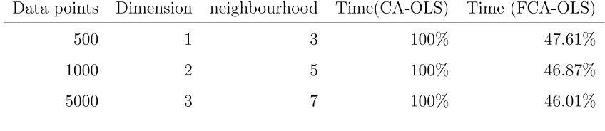
The detail of this algorithm is given in [19]. Table 1 shows that the new FCA-OLS

routine results in a significant reduction in the computational time.

Table 1: Comparison of computational cost

Data points Dimension neighbourhood Time(CA-OLS) Time (FCA-OLS)

500 1 3 100% 47.61%

1000 2 5 100% 46.87%

5000 3 7 100% 46.01%

2.6

Conclusions

The estimation procedures discussed above exploit the observation that binary CA rules

can be exactly represented as polynomial models which collapse to relatively simple forms

even for high-dimensional CAs. This transforms the problem from a

nonlinear-in-the-parameters to a linear-in-the -nonlinear-in-the-parameters formulation. The only information required

to initialise the algorithm is to set the range of the largest expected neighborhood over

which the algorithm searches for candidate model terms. The CA-OLS estimator then

searches through all the possible terms and discards all the redundant terms to yield the

final estimated model.

Several simulated examples in [27], [28] show the power of the new approaches and

demonstrate for the first time how polynomial CA models can be extracted from data

generated from deterministic, probabilistic and high-dimensional CA systems. The

sim-ulation examples in [19] show the proposed fast CA-OLS can improve the effectiveness

substantially, and this may assist further research into real-time identification for real

3

Neighbourhood Detection

3.1

Background and Motivation

In most former studies, the CA neighbourhood was manually predefined as the cells

that were immediately close to the cell to be updated. For example Richards directly

selected the Moore structure as the neighbourhood of the pattern generated by dendritic

solidification [21]. Adamazky set a minimal neighbourhood before the identification of

a one-dimensional CA [2]. But for most systems, especially higher order CA, it will

often be very difficult to manually choose a candidate neighbourhood that just covers

the exact neighbourhood and which rejects many possible redundant cells. Hence, the

detection of the significant neighbourhood before identifying the rule is a key step in CA

identification.

3.2

Neighbourhood Detection using CA-OLS

As shown in Sec.2, Yang and Billings proposed the CA-OLS to detect the neighbourhood

based on the polynomial realization (4) [27]-[28]. The preliminary step in this algorithm

involves choosing an initial candidate neighbourhood, which can be coarse but must be

large enough to include all correct neighbourhoods. Consider a one-dimensional CA

for example and assume the neighbourhood of the cell c(j;t) is chosen as {c(j −1;t−

1), c(j;t −1), c(j + 1;t −1)}, a polynomial model, expressed as equation (5), can be

generated according to equation (4).

c(j;t) = θ0+θ1c(j −1;t−1) +θ2c(j;t−1)

+θ3c(j+ 1;t−1) +θ4c(j−1;t−1)c(j;t−1)

+θ5c(j−1;t−1)c(j+ 1;t−1)

+θ6c(j;t−1)c(j+ 1;t−1)

+θ7c(j−1;t−1)c(j;t−1)c(j+ 1;t−1) (5)

Determining which terms are significant and which terms are redundant can be derived

directly from the Error Reduction Radio (ERR), which measures the contribution of each

candidate term to the updated cell, and which is part of the CA-OLS routine. Using

terms can then be discarded.

3.3

Neighbourhood Detection based on a Statistic

Mei and Billings [20] recently proposed a new neighbourhood detection routine, which

can refine the candidate neighbourhood according to a statistic associated with each

combination of candidate neighbourhood cells and the updated cell, and from which an

exact neighbourhood can be obtained.

The basis of this algorithm is to select a neighbourhood candidate set initially, which

must be large enough to include all potential neighbourhood cells. Then each cell in

the neighbourhood candidate set will be assessed according to the contribution made to

the cell to be updated. Consider a one-dimensional deterministic CA for example and

assume the neighbourhood of the cellc(j;t) is chosen asRk{c(j;t)}at iteration time step

k. The cells of the considered neighbourhood could be divided into two parts: confirmed

cells and unconfirmed cells. A series of data pairs can be collected as (Rk{c(j;t)}, c(j;t)).

Consider one of the unconfirmed cells inRk{c(j;t)}. If it is a redundant cell based on the

statistic of collected data pairs (see [20] for full details), this cell should be discarded and

the data pairs should be re-collected because of the change of candidate neighbourhood.

If it is a significant cell, the cell would be moved into the set of confirmed cells, and the

next unconfirmed cell would be considered. This procedure is repeated until all cells in

the candidate neighbourhood are confirmed.

3.4

Neighbourhood Detection using Mutual Information

All previous methods need an initial candidate set before neighbourhood detection can

commence and this must include all the correct neighbourhoods. This maybe difficult for

some unknown systems. To avoid this step, a new neighbourhood detection algorithm

was introduced by Zhao and Billings [31] based on mutual information (MI) to provide

an initial indication of the temporal and spatial range in the identification of CA. This

initial neighbourhood is then used to prime a FCA-OLS algorithm to find the correct

model terms and unknown parameters in a CA model. This provides a coarse-to-fine

re-duce the potential neighbourhood choices which are then optimised using the FCA-OLS

identification algorithm.

Consider the one-dimensional CA case to illustrate the approach and assume the

neigh-bourhood of the cell c(j;t) is {c(j − a1;t −b1), ..., c(j − an;t − bn)}. The aim is to

determine the maximal spatial lag an and the maximal temporal lag bn.

Definition 1 A case is defined as a pair of {f(R{j;t}), c(j;t)}, where R{j;t} is the

neighbourhood of a cell c(j) at time step t and the c(j;t) is the state value of the cell at time stept, andf(R{j;t}) = c1+2c2+..+2m−1c

m assumingR{j;t}={c1, c2, ..., cm}. For

example, if the state value of the updated cellc(j;t)is1and the state of its neighbourhood

R{j;t} is {0,1,1}, the case can be described as {5,1}.

Essentially, R{j;t} represents the input and the c(j;t) represents the output of a

non-linear system. If the candidate neighbourhood R{j;t} is large enough to cover all the

correct neighbourhoods, the mutual information between f(R{j;t}) with c(j;t) should

be close to 1. If R{j;t} can not contain all the correct neighbourhoods, the Mutual

Information between f(R{j;t}) with c(j;t) will be close to 0. Based on these results a

new criteria, which introduces MI as a fitness function to establish a measurement for

ranking each candidate neighbourhood was introduced in Zhao and Billings [31].

3.5

Conclusions

Three new neighbourhood detection methods have been derived for both deterministic

and probabilistic CA. Yang’s method directly selects the significant terms by the ERR

values, the by-product of CA-OLS, but the procedure can be time consuming if the

can-didate neighbourhood is large. Mei’s method allows the neighoubhood detection to be

decoupled from the CA rule determination by choosing the exact neighbourhood.

Es-sentially, this is a preliminary step before Yang’s method, which may save time when

implementing CA-OLS. Zhao’s method solves the problem of initial neighbourhood

se-lection and produces an exact neighbourhood as well.

Many simulation examples have been given in the corresponding papers to demonstrate

4

Identification of Excitable Media

4.1

Introduction

Excitable media systems, which were first introduced by Wiener and Rosenbluth in order

to explain heart arrhythmia caused by spiral waves [23], are now recognized as an

im-portant class of spatio-temporal dynamic systems. Examples of excitable media systems

include the Belousov-Zhabotinskii (BZ) reaction [16], waves of electrical stimulation in

heart muscles [25], autocatalytic reactions on metal surfaces [15], and the propagation

of forest fires [9].

Wiener introduced the notation ofrefractory state,excited state andexcitable state to in-vestigate excitable media. The defining characteristics of excitable systems are: starting

at a stable equilibrium (excitable state) a stimulus above a certain threshold generates a

burst of activity (excited state) followed by a refractory period. Due to the activity

ini-tiated by a supercritical perturbation, travelling excitation waves of various geometries

can occur, including ring and spiral waves.

In this section the focus is on developing algorithms which can be applied to determine

the neighbourhood and a representative model of excitable media from observations of

the spatio-temporal pattern and no other a priori information. The study begins with examples of excitable media behaviour to demonstrate that highly complex patterns, can

be generated from relatively simple models. A algorithm using mutual information is

then derived to determine the neighbourhood, the excitation threshold, and the number

of excitation states. Based on the above steps two methods of identifying the rule based

on a multimodel and a polynomial model representation are introduced.

4.2

Simulation of Excitable Media in CA

The Greenberg-Hasting Model(GHM), which was introduced by Greenberg and Hasting

[14], is the most common CA form of model for excitable media.

The GHM model γt is a very simple cellular automata that emulates an excitable media

[Robert, 1993]. At each timet, γt ∈ {0, ..., N −1}Z

d

. This means that for each x∈_Zd_,

γt(x) has one of N possible values 0, ..., N−1. The evolution of the GHM model can be

rule.

For the GHM, the commonly used type of lattice is the square lattice. The neighbourhood

structure varies depending on the construction of the model. Consider a two-dimensional

GHM as a CA for example. The neighbourhood could be a von Neumann structure, a

Moore structure or an Extended Moore structure [32].

The transition rule of a GHM can be determined by three parameters: the number N

of all available states; the number E of excited states; the threshold number T of sites

needed for excitation. Denoting the cell at position (x, y) at time step t as c(x;y;t).

The state c(x;y;t)(c(x;y;t) ∈ {0, ..., N − 1}) is an integer value, where 0 represents

an excitable state, 1, ..., E represent the excited states, and E + 1, ..., N −1 represent

the refractory states. Initializing each cell at time step 0, the GHM updates all cells

synchronously by Transition Rule 1 at each step.

Transition Rule 1 The transition rule of the GHM as a CA:

• if 1≤c(x;y;t)< N, then c(x;y;t+ 1) = (c(x;y;t) + 1) mod N

• if c(x;y;t) = 0, then c(x;y;t+ 1) = 1 when #(Rc(x;y;t))≥T, else c(x;y;t+ 1) = 0

(Rc(x;y;t)denotes the neighbourhood ofc(x;y;t),#(R)denotes the number of excited

sites in R)

Using this simple rule, different complex patterns can be generated using different initial

values or parameters. Figure 1 shows an example generated by GHM.

4.3

Identification of Excitable Media

There are two parameters that need to be determined during the identification of

ex-citable media: the neighbourhood and the transition rule. In the following sections

algorithms to detect the neighbourhood and to identify the rule will be discussed.

4.3.1 Neighbourhood detection

For most systems, especially high dimensional CA, it will be very difficult to manually

select an appropriate candidate neighbourhood that just covers the exact neighbourhood

(a) t=1 (b) t=10 (c) t=12 (d) t=14

(e) t=16 (f) t=18 (g) t=20 (h) t=22

Figure 1: Evolution of a GHM as a CA on a 60× 60 square lattice with an Extended Moore

neighbourhood(r_{= 2), and} N_{= 7,} E_{= 1 and}T _{= 3.}

such as excitable media systems. If an incorrect neighbourhood is selected, it will

ei-ther be impossible to find the correct model or the model will be over parameterized

and computational time will increase dramatically. Based on the special properties of

excitable media, a new neighbourhood detection approach has been introduced based on

mutual information, which can not only determine the neighbourhood but also estimate

the number E of excited states [32].

The neighbourhood detection procedure can be briefly summarized by the following

steps.

Initially select the candidate neighbourhood as the von Neumann neighbourhood and select E as 0.

1. Threshold all the observed patterns to create a binary pattern using the current

E.

2. Scan all the binary patterns and calculate the value of the mutual information.

3. Increase E and repeatsteps 1 and 2 untilE =n, where n denotes the number of current candidate neighbourhood cells.

structureto theMoore structureor from theMoore structureto theExtended Moore structure (r= 2) and reset E to 0. Then repeatsteps 1 to 3 until a peak value of mutual information appears. The candidate neighbourhood and E with maximal

mutual information can be determined as the final results.

4.3.2 Rule identification

Two types of models, the multiple model and the polynomial model, can represent the

transition rule of excitable media, and algorithms for the identification both of these

have been proposed.

Rule identification using a multiple model: The advantage of this type of model is

the principle of the evolution can easily be understood and it is not difficult to simulate

the model. The evolution of a GHM is determined by four parameters: the

neighbour-hood; the number N of all available colours; the number E of excited colours; and the

threshold number T of sites needed for excitation. The selection of the neighbourhood

and E have been described using mutual information above, and only N and T are

un-known parameters. The estimation ofN can often be ignored here because the evolution

of a GHM mainly depends on the excitation from excitable cell to excited cell, and it is

not important how many refractory states exist. The threshold number T therefore is

the only parameter needed to be estimated in this step. The detail about how to identify

T can be found in [32].

Rule identification using a polynomial model: The main advantage of the

poly-nomial model form is that it is much easier to analyse and validate than the multiple

model. After generating binary frames using the detected value of E, the identification

of the rule using a polynomial representation can be summarized as:

1. Collect the input-output cases{xi;yi}, i∈ {1, ..., M}using the detected

neighbour-hood and E, where

xi ={c(x−a1;y−b1;t−1), c(x−a2;y−b2;t−1), ..., c(x−an;y−bn;t−1)}

yi =c(x;y;t)

(6)

M denotes the number of collected cases and n denotes the number of

2. Apply the Orthogonal Least Squares (OLS) algorithm for CA to estimate the

parameters of Eq. (4) using the collected data set {xi;yi}.

4.4

Identification of a Belousov-Zhabotinsky Reaction using

CA Models

4.4.1 Introduction

The Belousov-Zhabotinsky (BZ) chemical reaction, named after B.P.Belousov who first

discovered the reaction [10] and A.M.Zhabotinsky who continued Belousov’s early work

[29], is a famous experiment in excitable media. Once the reaction gets started grey

rings and spirals can be seen propagating from localized regions on a red background. A

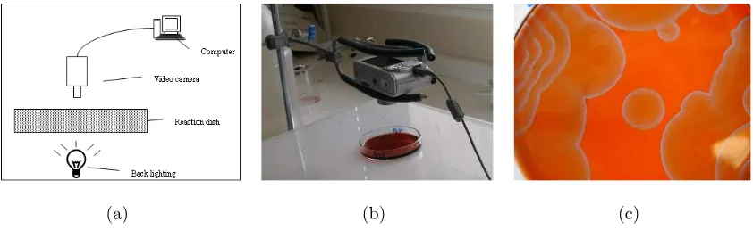
snapshot of a typical pattern is shown in Fig.2.(c), where the wave fronts of the observed

patterns appear to be quite similar to those of the simulated patterns using the GHM,

especially the pattern shown in Fig.1.

In this section the identification of a model of a real BZ reaction using a CA model

(a) (b) (c)

Figure 2: (a) Schematic of the data acquisition setup; (b) Photo of acquiring device ; (c)A snapshot of

an acquired pattern

directly from sampled data will be studied. The focus of the section will be on the

prac-tical aspects of imaging a real BZ reaction and the identification of dynamic models of

4.4.2 Data acquisition and pre-processing

The chemical processor was prepared in a thin layer BZ reaction using a recipe adapted

from Field and Winfree [24]. The experimental apparatus of acquisition is illustrated

by Fig.2.(a). To acquire the high quality images a digital camera, which was fixed by

a bracket and connected to the computer directly using the USB socket as shown in

Fig.2.(b), was used. The images were acquired with 640×480 pixel resolution where

each pixel had a 24bit colour-scale value. Before identification the acquired raw data

must be pre-processed to reduce noise and must then be mapped onto a lattice based

on the three components of CA, which involves the calibration of the pixel size and the

calibration of the number of colours. The detail of these steps can be found in [33].

4.4.3 Rule identification

Region selection: In most recent studies of excitable media the evolution of the

pat-tern is assumed to be uniform so that each cell in the patpat-tern has the same transition

rule. This may not hold for a real system because there may be noise introduced by

data acquisition which could make the rule change. Hence, it is necessary to select an

appropriate region of the image which has a uniform or nearly uniform rule. A method

was proposed in [33] which divides the image into ns squares, and then estimates the

threshold number T in the GHM of each part. Normally, ns was chosen as 64 for a raw

image with 640×480 pixels. Part of the image can then be chosen as the sample area

where the rule is assumed to be uniform based on the generated rule distribution graph.

Rule identification: The identification of the rule for the considered region of the BZ

reaction is the same as the method for excitable media.

Model evaluation: To evaluate the identified models visually and quantitatively, One

Step Ahead (OSA) predictions were compared with the recorded data. Figure

3.(a)-(c) visually shows the 10,50,80 time step OSA predictions using the identified multiple

model, and Fig.3.(d)-(f) show the 20,60,100 time step OSA predictions using the

iden-tified polynomial model. Both these clearly demonstrate the diffusion characteristics of

the BZ patterns. To quantitatively access the performance of the obtained CA rules we

can compare the results of the predictions from the identified models to the actual BZ

(a) 10 steps (b) 50 steps (c) 80 steps

(d) 20 steps (e) 60 steps (f) 100 steps

Figure 3: (a)-(c):OSA predictions using the identified GHM; (d)-(e):OSA predictions the identified

polynomial model

into account the correct and false cell predictions for the excited state and refractory

state, and the correct and false cell predictions for the excitable state are used. Full

details of these procedure can be found in [33].

4.5

Conclusions

New methods of extracting mathematical models of CA directly from real imaged data

from a BZ reaction has been presented. A procedure which maps the digital image to

a latticed CA pattern has been proposed. New methods of synthesizing the horizontal

and vertical calibration were introduced, together with the edge purging procedure to

remove the gradient between the wave fronts and the background. A new region selection

approach has also been proposed, and procedures for the identification of two CA model

types, the GHM and the polynomial model, have been described. A comparison of the

results are very encouraging. The identified models can reproduce the patterns with

similar dynamic features compared to the actual BZ reaction.

Identification of real reaction systems is often very difficult because of the many factors

involved. Moreover, natural data will always be slightly corrupted by the imaging devices

during data acquisition. The results in the section represent preliminary results and

many more experiments need to be conduced and all aspects of the data collection and

modelling of this complex class of system require further study.

5

Identification of Hybrid Cellular Automata using

Segmentation Methods

Most previous investigations of CA have concentrated on uniform cellular automata, or

CA where the transition rule is identical at all positions over the whole lattice and at

all times during the evolution. However, when studying an unknown real system, it

may be unwise to assume that the rule representing the system is homogeneous over the

whole image. Hence, recently, the application of hybrid cellular automata has attracted

more and more investigations [11]-[13], which try to represent a complex system using

multi-rules. However, very few of these methods can solve the inverse problem - that is

identifying the hybrid cellular automata rule given the observed data.

This section introduces a new method for the identification of hybrid CA which initially

simplifies the problem from hybrid CA to uniform CA by partitioning the regions based

on the rules by employing the segmentation methods. Then the methods described in

previous sections can be applied for the identification of CA with a uniform rule in each

separate region to obtain the final hybrid rule or model.

The procedure of transferring the identification of hybrid CA to the identification of

uniform CA can be summarized by the steps in the following sections.

5.1

Map the realistic CA pattern to a virtual image.

An image is composed of pixels on a lattice, and a CA is composed of cells on a lattice,

which makes the possibility of applying segmentation methods from image processing to

The key step is that a pixel in a virtual image can be created by mapping a rectangular

region with size nb × nb in the CA pattern, and this will be refereed to as a block.

Consider a CA pattern on a nx×ny lattice, a virtual image with n_nx

b ×

ny

nb pixels could be generated by setting the size of block asnb. The selection ofnb is important because

if nb is selected to be too large, then obviously the segmentation would be less accurate

and the probability of multi-rules in one block may be large. This in turn could lead

to the difficulty in calculating the property of the block. If nb is selected too small, the

sample data for calculating the property of the block will be less, which could make the

result over-estimated.

The method proposed in this section introduces a parameter namedTu, which represents

a noise-immune ability. Consider a block which has n rules denoted by r1, r2, ..., rn. If

there is a rule ri whose percent of occupancy in that block is larger than Tu, this block

will be marked as obeying ri. If there is no such rule, this block should be marked as

unidentifiable. Obviously, Tu should be chosen between 0.5 to 1. The smaller Tu is, the

more probability there is of identifying the block, but there is more risk of getting a

wrong rule. Hence, there is a clear tradeoff between the accuracy of segmentation and

the property calculations, and a tradeoff in the block property between the accuracy and

the identifiability. The crucial step of the mapping procedure is how to calculate the

property of each block in a CA pattern. The detail of this method could be found in

[34]. Finally, the mapping procedure between the pattern of hybrid CA and the virtual

image can be summarized as:

Consider a nx ×ny hybrid CA pattern and denote the selected block size as nb. If the

currently considered block is identifiable, the property of the considered pixel in the image is assigned the value Pv of the corresponding block. If the block is unidentifiable, the

property of the corresponding pixel in the image should be assigned a special value, such as 0. The size of the mapped virtual image would be nx

nb ×

ny

nb.

5.2

Region Segmentation

Two popular image segmentation methods are introduced in the following sections to

assist the identification of hybrid CA by partitioning the generated virtual image into

The objective of segmentation is to partition an image into regions. This section

dis-cusses the segmentation techniques that are based on finding the regions directly. Let

R represent the entire image region. The segmentation may be viewed as a process that

partitions R into n subregions, R1, R2, ..., Rn, such that

(a) Sn_i=1Ri =R,

(b) Ri is a connected region, i= 1,2, ..., n,

(c) Ri∩Rj =φ for all iand j, i6=j

(d) P(Ri) = TRUE for i= 1,2, ..., n,

(e) P(Ri∪Rj) = FALSE for i≤j,

(7)

where P(Ri) is a logical predicate defined over the points in set Ri, and φ is the null

set. Condition (a) indicates that the segmentation must be complete; that is, every

pixel must be in a region. The second condition requires that points in a region must

be connected. Condition (c) indicates that the regions must be disjoint. Condition (d)

deals with the properties that must be satisfied by the pixels in a segmentation region.

In the current application, P(Ri) =T RU E implies the pixels in the region Ri have the

same properties. Finally, condition (e) indicates that regions Ri and Rj are different in

the sense of predicateP.

5.2.1 Region Growing

Region growing is a well known technique for image segmentation. It postulates that neighbouring pixels within the same region have similar intensity values. The general

idea ofregion growing is to group pixels with the same or similar intensities to one region according to a given homogeneity criterion. More precisely, region growing starts with a set of pre-specified seed pixel(s) and grows from these seeds by merging neighbouring

pixels whose properties are most similar to the pre-merged region. Typically, the

ho-mogeneity criterion is defined as the difference between the intensity of the candidate

pixel and the average intensity of the pre-merged region. If the homogeneity criterion is

satisfied, the candidate pixel will be merged to the pre-merged region. The procedure is

iterative: at each step, a pixel is merged according to the homogeneity criterion. This

process is repeated until no more pixels are assigned to this region. The homogeneity

5.2.2 Region Splitting and Merging Method

The procedure discussed in the previous section grows regions starting from a given set

of seed pixels. An alternative is initially to subdivide an image into a set of arbitrary,

disjoined regions and then merge and/or spit the regions in an attempt to satisfy the

conditions stated in Equation (7). A region splitting and merging algorithm that itera-tively works toward satisfying these constraints is explained as follows.

LetRrepresent the entire image region and select a predicateP as discussed in Equation

(7). For a hybrid CA, P(Ri) =TRUE means all the cells in Ri have the same CA

tran-sition rule. Assume a square image, one approach for segmentation of R is to subdivide

it successively into smaller and smaller quadrant regions such that, for any region Ri,

P(Ri) =TRUE. That is, if P(Ri) =FALSE, the image is divided into quadrants. If P is

FALSE for any quadrant, that quadrant is subdivided into sub-quadrants, and so on.

5.2.3 Removing noise

A popular nonlinear filter in image processing called the median filter can be employed to remove noise in the segmented image. The Median filter replaces the considered pixel value by the median of the values in a neighbourhood of that pixel. This method is

particularly effective when the noise pattern consists of strong, spike-like components.

Whennb is chosen small, there could be some blocks which can not be identified because

the number of measurements is small compared to the number of possible discrete states.

For this reason, the segmented image could include salt-pepper noise. Median filtering

can remove this kind of noise effectively.

5.3

Conclusions

Some examples, including one-dimensional CA and two-dimensional CA, have been

em-ployed to evaluate this method [34]. It is shown that the results are encouraging by

comparing the original rule distribution graph and the detected rule distribution graph,

and comparing the comparison the reconstructed patterns and the observed patterns.

Moreover, the hybrid cellular automata could be more complex than what is described

in this paper. For example, the rule could be changed in the same position following the

are required to deal with the more complex cases which could occur in the real systems.

Acknowledgment

The authors gratefully acknowledge that part of this work was financed by EPSRC(UK).

We are very grateful to Alex Routh, Department of Chemical Engineering, University

of Sheffield who set up and conducted the real experiment. We would also like to thank

A.Adamatzky for the kind invitation to write a paper reviewing the results developed at

Sheffield.

References

[1] Adamatzky, A. [1994]Identification of Cellular Automata(Taylor Francis, London).

[2] Adamatzky, A. [1997] ”Automatic programming of cellular automata: identification

approach,” Kybernetes 26 (2-3): 126-133.

[3] Adamatzky, A. [2001] Cellular Automata: a discrete university (World Scientific, London).

[4] Adamaskiy, A & Bronnikov, V. [1990] ”Identification of additive cellular automata,”

Soviet journal of computer and systems sciences 25(5), 47-51.

[5] Adamaskiy, A. [1991] ”Identification of fuzzy cellular automata,” Avtomatika I vy-chislitelnaya tekhnaika 6, 75-80.

[6] Adamaskiy, A. [1992] ”Identification of probabilistic cellular automata,”Soviet jour-nal of computer and systems sciences 30(3), 118-123.

[7] Adamaskiy, A. [1992] ”Complecity of identification of cellular automata,” Automa-tion and remote control 53(9), 1449-1458.

[8] Andersson, C., Rasmussen, S. & White, R. [2002] ”Urban settlement transitions,”

Enviroment and Planning B-Planning and Design 29(6), 841-865.

[9] Bak, P., Chen, K. & Tang, C. [1990] ”A forest-fire model and some thoughts on

[10] Belousov, B. P. [1958] ”A Periodic Reaction and Its Mechanism,”Sbornik Referatov po Radiasionni Meditsine, Moscow.

[11] Cattell, K. & Zhang, S. [1999] ”2-by-n Hybrid Cellular Automata with Regular

Configuration: Theory and Application”,IEEE Transactions on Computers 48(3), 285-295.

[12] Chaudhuri, P.P., Chowdhury, D. R., Nandi, S. & Chattopadhyay, S. [1997] Additive Cellular Automata: Theory and Applications (IEEE Computer Society Press).

[13] Corno, F. & Maurizio, R. [2000] ”Low Power BIST via Non-Linear Hybrid Cellular

Automata”, Proceedings of the 18th IEEE VLSI Test Symposium (VTS’00), pp.29.

[14] Greenberg, J. M., Hassard, B. D. & Hastings, S. P. [1978] ”Pattern

forma-tion and periodic structures in systems modeled by reacforma-tion-diffusion equanforma-tions”,

B.Am.Math.Soc. 84, 1296-1327.

[15] Gerhardt, M. & Schuster, H. [1989] ”A cellular automaton describing the formation

of spatially ordered structures in chemical systems,”Physica D. 36, 209-221.

[16] Jahnke, W., Skaggs, W. E. & Winfree, A. T. [1989] ”Chemical vortex dynamics in

the Belousov-Zhabotinskii reaction and in the two-variable Oregonator model,” J. Phys. Chem.93, 740-749.

[17] Li, X.B., Jiang, R. & Wu, Q.S. [2003], ”Cellular automata model simulating complex

spatiotemporal structure of wide jams,” Physical Review E, 68(1) Part2.

[18] Maeda, K. & Sakama, C. [2003] ”Discovery of Cellular Automata Rules Using

Cases,”Discovery science, Proceedings lecture notes in artificial intelligence 2843, 360-368.

[19] Mei, S.S. & Billings, S.A. [2005] ”A New Fast Cellular Automata Orthogonal Least

Squares Identification Method,”International journal of system science 36(8), 491-499.

[20] Mei, S.S., Billings, S.A. & Guo, L.Z. [2005] ”A Neighbourhood selection method for

[21] Richards, F.C. [1990] ”Extracting cellular automata rules directly from experimental

data,” Phys.D, 45,189-202.

[22] Sanchez, J.R. [2004] ”Pattern recognition of one-dimensional cellular automata using

Markov chains,” International journal of modern physics C 15(4), 563-567.

[23] Wiener, N. & Rosenbluth, M. [1946] ”The mathematical formulation of the problem

of conduction of impulses in a network of connected excitable elements, specifically

in cardiac muscle,” Archos. Inst. Cardiol. Mex. 16, 205-265.

[24] Winfree, A. T. [1972] ”Spiral waves of chemical activity,”Science, 175, 634-636.

[25] Winfree, A. T. [1989] ”Electrical instability in cardiac muscle: phase singularities

and rotors,” J. Theor. Biol. 138, 353-405.

[26] Veronique, T. [1999] ”Two-dimensional cellular automata recognizer,” Theoretical Computer Science 218, 325-346.

[27] Yang, Y.X. & Billings, S.A. [2003] ”Identification of probabilistic cellular automata,”

IEEE Transactions on systems Man and Cybernetics Part B 33(2), 225-236.

[28] Yang, Y.X. & Billings, S.A. [2003] ”Identification of the neighbourhood and CA

rules from spatio-temporal CA patterns,” IEEE Transactions on systems Man and Cybernetics Part B 30(2), 332-339.

[29] Zhabotinskii, M. [1964] ”Periodic Kinetics of Oxidation of Malonic Acid in Solution

(Study of the Belousov Reaction Kinetics),” Biophys 9, 306-311.

[30] Zhang, Q, ”Using wavelet network in non parametric estimation,” IRISA, France,

Publication Interne, 32p.

[31] Zhao, Y. & Billings, S.A. [2006] ”Neighborhood Detection Using Mutual Information

for the Identification of Cellular Automata”, IEEE Transactions on systems Man and Cybernetics Part B 36(2), 473-479.

[32] Zhao, Y., Billings, S.A. & Routh, A. [2005] ”Identification of Excitable Media using

[33] Zhao, Y, & Billlings, S.A. [2006] ”Identification of the Belousov-Zhabotinsky

Re-action using Cellular Automata Models,” International journal of bifurcation and chaos, accepeted.

[34] Zhao, Y. & Billlings, S. A. [2006] ”Identification of Hybrid Cellular Automata

us-ing Image Segmentation Methods,”Report of department of Automatic Control and Systems Engineering, University of Sheffield, 936.

[35] Zhu, Q.M. & Billings, S.A. [1996] ”Fast identification of linear stochastic models