Power Generation for a 2D Tethered Wing Model with a Variable Tether Length

(1)

Theses Thesis/Dissertation Collections

8-2014

Power Generation for a 2D Tethered Wing Model

with a Variable Tether Length

Ashwin Chander Ramesh

Follow this and additional works at:http://scholarworks.rit.edu/theses

This Thesis is brought to you for free and open access by the Thesis/Dissertation Collections at RIT Scholar Works. It has been accepted for inclusion in Theses by an authorized administrator of RIT Scholar Works. For more information, please [email protected].

Recommended Citation

(2)

Power Generation for a 2D Tethered Wing

Model with a Variable Tether Length

by

A Thesis Submitted in Partial Fulfillment of the Requirements for the Degree of Master of Science

in Mechanical Engineering

Supervised by

Assistant Professor Dr. Mario W. Gomes Department of Mechanical Engineering

Kate Gleason College of Engineering Rochester Institute of Technology

Rochester, New York August 2014

Approved by:

Dr. Mario W. Gomes, Assistant Professor

Thesis Advisor, Department of Mechanical Engineering

Dr. Agamemnon Crassidis, Associate Professor

Committee Member, Department of Mechanical Engineering

Dr. Steven Day, Associate Professor

Committee Member, Department of Mechanical Engineering

Dr. Wayne Walter, Professor, PE

(3)

Rochester Institute of Technology Kate Gleason College of Engineering

Title:

Power Generation for a 2D Tethered Wing Model with a Variable Tether Length

I, Ashwin Chander Ramesh, hereby grant permission to the Wallace Memorial Library to reproduce my thesis in whole or part.

(4)

iii

(5)

Acknowledgments

The Master’s degree at RIT has been a great experience and an amazing journey for

me. Firstly I would like to thank my family who have always stood by me. I would

like to thank my mother Shanthi who has guided me with advice and encouraged

me to pursue my every dream, my sister Sanju who makes my day by having long

conversations with me and making me feel like I’m back home for the time I am

talking to her.

The completion of the thesis could not be possible without the support of the Dr.

Gomes. Working with you has been a life changing experience for me. I have learned

a lot of things from you, not only academic but also real life lessons. I am very glad

I met you and you have been a great influence on me. Thank you for being patient

with me and guiding me through any and all problems.

I would also like to thank my committee members Dr. Crassidis and Dr. Day

for all your help with my research and academic progress. The faculty at Mechanical

Engineering are really great, and I thank them for teaching me everything that I have

learned over the past two years. Without this knowledge I would likely not have been

able complete my thesis successfully.

I would like to thank Jill, Diane, Diedra and Hillary for always welcoming me at the

ME office with a nice smile and all your help with the scheduling, room reservation,

registration and all other academic paper work. Bill thank you for all the software,

and computer support that you have provided over the past two years and hiring me

to work as a labbie. Mostly I thank everyone for being a good friend.

(6)

v

Bill, Paul, Kyle, Saj and all the other students who have worked in the Energy and

Motion Lab. Energy and Motion Lab has been my second home at Rochester for more

than a year and my labmates have been like family to me. You guys have always

been available for me when I needed you and all your inputs at lab meetings were

very helpful to me. I sincerely hope we continue to stay in touch, and bounce ideas

(7)

Abstract

Power Generation for a 2D Tethered Wing Model with a Variable Tether

Length

Supervising Professor: Dr. Mario W. Gomes

Airborne wind energy systems consist of a lifting body and a tether. Several airborne wind energy systems have been created by others, but the most promising consists of a wing which translates through the air in a crosswind motion. Two computational models of a translating wing system were used to study the dynamics and performance of these systems. The first model that was examined consists of a rigid connecting arm between a rotating base station and a wing. A study of this model showed that one can increase the power production of the system by changing the wing angle relative to the connecting arm during motion. Using a variable relative wing angle, an average power of 7.7W is generated which is an increase of 30% over the fixed wing angle system.

(8)

B.1 2D and 3D lift and drag coefficients [7]. This model uses steady state lift and drag coefficients. McConnagy et al. analyzed these experimen-tal values of lift and drag coefficients for a range of Reynolds numbers (104_to107_{) [16] and observed that the lift and drag coefficients selected} hold good for this range. . . 134

B.2 Initial conditions for the first phase of the CLRS . . . 135

B.3 Initial conditions for the second phase of the CLRS . . . 135

B.4 Initial conditions for the second phase of the CLRS . . . 138

B.5 Initial conditions for the fourth phase of the CLRS . . . 140

B.6 Initial conditions for the first phase of the RRS . . . 146

B.7 Initial conditions for the second phase of the RRS . . . 147

(12)

List of Figures

1.1 Average wind-speed over the Netherlands over 20 years. Image taken from [13] . . . 6 1.2 The wind power density profiles at the five largest cities in the world.

Image taken from [3] . . . 7 1.3 Wind power density comparison for land versus sea at different

alti-tudes. Image taken from [3] . . . 8 1.4 A sketch of the design of ’Charvolant’ -a kite drawn carriage. Image

taken from [17] . . . 10 1.5 A sketch of the carriage being powered by a kite . Image taken from [17] 11 1.6 Density of effective area of added drag affects global KEE. Image taken

from [15] . . . 12 1.7 Atmospheric kinetic energy deceases with increase in KEE. Image taken

from [15] . . . 13 1.8 The production rate of atmospheric kinetic energy increases with

in-crease in KEE. Image taken from [15] . . . 13 1.9 Kitegen para-foils reaches altitudes of about 1000m and tethered to a

spinning carousel at the ground. Image taken from [3] . . . 16 1.10 Kitegen para-foils reaches altitudes of about 1000 mand tethered to a

spinning carousel at the ground. Image taken from [3] . . . 17 1.11 Flying electric generators by Sky Windpower. Tethered rotor-crafts

reaches altitudes of 10,000 m. Image taken from [3] . . . 18 1.12 Kitegen para-foils reaches altitudes of about 1000 m and tethered to a

spinning carousel at the ground. Image taken from [3] . . . 18 1.13 Flying electric generators by Sky Windpower. Tethered rotor-crafts

reaches altitudes of 10,000 m. Image taken from [3] . . . 19 1.14 Forces and velocities on a weightless simple kite. Image taken from [14] 21 1.15 Forces and velocity vectors on a mass-less kite during the crosswind

motion. Image taken from [14] . . . 21 1.16 Comparison of the power obtained in the three cases with a fixed L/D

ratio kite. Image taken from [14] . . . 23 1.17 Forces acting on a kite during ascent. Image taken from [10] . . . 25

(13)

1.18 Variation of average power with load during ascent.Image taken from [10] . . . 26 1.19 Instantaneous power during the descent.Image taken from [10] . . . . 27 1.20 Normalized instantaneous power for different loads during ascent.Image

taken from [10] . . . 27 1.21 Drag flaps used for steering stability. Image taken from [13] . . . 29 1.22 Servos located under the kite for control of angle of attack. Image

taken from [13] . . . 30 1.23 Control mechanism for the tether attachment point on the kite. Image

taken from [13] . . . 30 1.24 2D model of a kite with the bridle angle,azimuth angle,lift force and

center of pressure. Image taken from [19] . . . 32 1.25 Basic system diagram. Image taken from [19] . . . 32 1.26 Equilibrium altitude increases with increase in wind velocity. Image

taken from [19] . . . 33 1.27 Simplified representation of a tethered kite system with a moving

ground vehicle. Image taken from [24] . . . 35 1.28 Nominal system parameters. Image taken from [24] . . . 36 1.29 Optimal kite trajectories for low and high wind speeds.[24]. Image

taken from [24] . . . 38 1.30 Power generated increases with increase in cycle time.[24]. Image taken

from [24] . . . 39 1.31 Variation of azimuth angle ψ and the zenith angle φ at the ground

station .Image taken from [21] . . . 41 1.32 Pitching moment of the Kiteplane. Image taken from [21] . . . 42 1.33 Lift and Drag forces acting on the left and right wing. Image taken

from [21] . . . 42 1.34 zenith and pitch equilibrium. Image taken from [21] . . . 43 1.35 symmetric 2D motion of the Kiteplane. Image taken from [21] . . . . 43

2.1 The free body diagram rigid boom model . . . 47 2.2 The schematic of the rigid boom model . . . 48 2.3 The schematic view for the fixed beta system during the deploy stroke 50 2.4 The schematic view for the variable beta system during the deploy stroke 50 2.5 Average power as a function of beta to find the right parameter to

(14)

xiii

2.6 Average power as a function of generator constant to find the right value to maximize power production while keeping the beta fixed at 52◦_{. 57}

2.7 Fixed beta system . . . 57 (a) The acngular position attains periodicity with time for a fixed

beta system. . . 57 (b) The angular velocity attains periodicity with time for a fixed beta

system. . . 57 2.8 The system transitioning from transient to the steady-state can be

noticed for a fixed beta system. . . 58 2.9 The beta value which generated the highest torque is chosen as optimal

for a range 0◦

≤β _≤360◦_{. . . .} ₅₉

2.10 Surface plot showing the optimal beta values to maximize torque at the pivot point of the rigid boom system. . . 60 2.11 Contour plot for optimal beta values as a function of angular position

and angular velocity. . . 61 2.12 Variable beta system . . . 62

(a) Change in angular position for a variable beta system. The ac-ngular position attains periodicity with time for a variable beta system. . . 62 (b) Change in angular velocity for a variable beta system. The

ac-ngular velocity attains periodicity with time for a variable beta system. . . 62 2.13 Beta changes with time to maximize torque at every time step to

in-crease average cycle power . . . 63 2.14 The phase plane showing both transient and steady-state phases for

variable beta. This system reaches steady state over time. . . 64 2.15 Optimal generator constant for variable beta system . . . 65

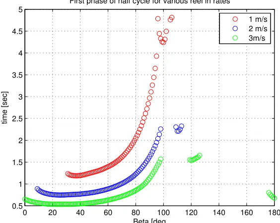
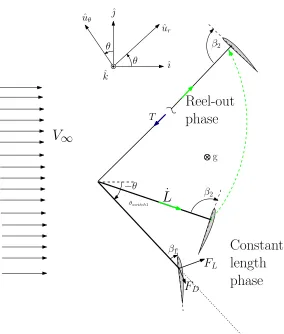
3.1 The schematic view for a half cycle of the variable tether length . . . 68 3.2 Time taken to reach a desired angular velocity for various beta values

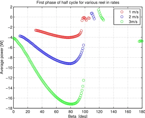
during the reel-in phase . . . 73 3.3 Energy consumed for variousβ values and reel-in rates . . . 74 3.4 Average power for variousβ values and reel-in rates during the reel-in

(15)

3.5 Instantaneous power for the half-cycle of the variable tether system. Power is consumed by the system during the reel-in phase and gen-erated during the reel-out phase. The negative power shown on the graph is when the system consumes power. . . 75 3.6 Tension force is proportional to the instantaneous power produced

dur-ing the reel-out phase . . . 75

4.1 The schematic view of the deploy stroke showing phases one and two of the CLRS . . . 79 4.2 The schematic view of the return stroke showing phases three and four

of the CLRS . . . 80 4.3 The schematic view of the final phase of one set for CLRS . . . 80 4.4 The schematic view of the CLRS showing three cycles which comprise

a single set . . . 81 4.5 Five different beta values chosen for the five phases in one set for the

CLRS . . . 83 4.6 The change from the constant-length and reel-out phases can be seen

noticed with change in length for the CLRS. The constant-length, reel-out and retraction phases can be seen. . . 83 4.7 The fluctuation in angular velocity with tether length for the CLRS . 84 4.8 Phase plane plot for third set of the CLRS. The three distinct curves

represent the three cycles of the system in each set. . . 84 4.9 Instantaneous power for the third set of the CLRS . . . 85 4.10 A closer view of the instantaneous power for the third set of the CLRS

showing the constant length, reel-out and the retraction phases. Power is not generated during the constant-length phase, generated during the reel-out phase and consumed by the system for the retraction phase. 86 4.11 Instantaneous for the three cycles of one set without the retraction phase. 87 4.12 Relative velocity for the third set of the CLRS. The relative velocity

increases resulting in higher peaks with time, because of the change in tether length with time. . . 88 4.13 Variation of the relative velocity with angular position for the CLRS.

The relative velocity reduces at the end of each stroke. . . 88 4.14 Analyzing the bridle angle to locate a local maximum of average power

(16)

xv

4.15 Analyzing the θswitch to locate a local maximum of average power for

the CLRS system. The θswitchis a crucial control parameter as it is the

angular position at which the system transitions between the constant-length phase and the reel-out phase. . . 90 4.16 Analyzing the beta for the reel-out phases to locate a local maximum

of average power production for the CLRS . . . 91 4.17 Analyzing the reel-out rates for the CLRS to locate a local maximum

of average power production . . . 91 4.18 The schematic view of the deploy stroke showing phases one and two

for RRS . . . 93 4.19 The schematic view of the return stroke showing phases three and for

the RRS . . . 94 4.20 Five different beta values chosen for the five phases in a cycle of the

RRS . . . 96 4.21 Change in length of the tether during the reel-in and reel-out phases

of the RRS . . . 97 4.22 The phase plane plot for the third set of the system of the RRS . . . 97 4.23 Instantaneous power for the third set of the RRS . . . 98 4.24 Closer look at the instantaneous power for the last set of the RRS.

Positive power is generated when the tether is reeled out and power is consumed by the system when the tether is reeled in . . . 99 4.25 Change in length of the tether during the reel-in and reel-out phases

of the RRS. The three distinct curves represent the three cycles in a set. . . 100 4.26 Analyzing the bridle angle for the reel-in phase to locate a local

maxi-mum of average power for the RRS . . . 101 4.27 Analyzing the bridle for the reel-out phases to locate a local maximum

of average power production for the RRS . . . 101 4.28 Analyzing the various reel-in rates for the reel-in phase to locate a local

maximum of average power production for one set of the RRS . . . . 102 4.29 Analyzing the reel-out rates for the RRS to locate a local maximum of

average power . . . 102 4.30 Analyzing the θswitch to locate a local maximum of average power for

the RRS. The θswitch is a crucial control parameter as it is the angular

(17)

B.1 Choosing the optimal control parameter for the first phase of the reel-out system . . . 136 (a) Searching for the optimal beta to minimze time consumed . . . 136 (b) Analysing the angular velocity of the system at the end of the

first phase as a function of time . . . 136 (c) Analyzing the angular velocity of the system for diferrent bridle

angles . . . 136 B.2 Analyzing a close range of control parameters for the second phase . . 138

(a) Analyzing averge power as a function of reelout rates and beta angles . . . 138 (b) Analyzing averge power as a function of reelout rates and beta

angles . . . 138 B.3 Analyzing reel-out rates while keeping beta fixed at 98◦ _{for the second}

phase to maximize power production . . . 139 (a) Average power produced during the secon phase while keeping

the bridle fixed . . . 139 (b) Checking the angular velocity of the system at the end of the

second phase for various reel-out rates while keeping the bridle fixed. . . 139 B.4 Analyzing different beta angles while keeping the reel-out rate fixed a

4m/s during the second phase . . . 139 (a) Analyzing the range of beta angles to maximize power production

for the second phase . . . 139 (b) Checking the angular velocity of the system at the end of the

second phase for various beta angles while keeping the reel-out rates fixed . . . 139 B.5 Selecting the optimal beta for the third phase of the reel-out system . 141

(a) Average power produced during the third phase for a range of bridle angles . . . 141 (b) Angular velocity reached at the end of the third phase as a

func-tion of the time consumed . . . 141 (c) Angular velcoity reached at the end of the third phase for a range

of beta angles . . . 141 B.6 Analyzing averge power as a function of reelout rates and beta angles 142 B.7 Analyzing a range of beta values while keeping the reel out rate fixed

(18)

xvii

(a) Average power produced during the fourth phase while keeping the reelout rate fixed for a range of beta . . . 143 (b) The angular velocity reached at the end of the phase for a range

of beta values . . . 143 B.8 Analyzing a range of reel-out rates while keeping the beta fixed at ₋98◦₁₄₃

(a) Average power produced for a range of reel-out rates while keep-ing the beta constant . . . 143 (b) Angular velocity of the system at the end of the fourth phase for

a range of reel-out rates . . . 143 B.9 Optimizing the control parameters for the first phase of the

reel-in-reel-out system . . . 145 (a) The variation in power used for the first phase for diferrent reel

in rates and bridel angle . . . 145 (b) A closer view of the variation in bridle angle between 0◦ _{and 80}◦ ₁₄₅

(c) The time taken to reach the predefined angular position for di-ferrent control parameters are analysed . . . 145 (d) A closer view of the variation in bridle angle between 0◦ _{and 80}◦ ₁₄₅

B.10 Analyzing optimal control parameters for the first phase . . . 146 (a) Analyzing optimal control paramters for the first phase for a

small range as a function of power . . . 146 (b) Analyzing optimal control paramters for the first phase for a

small range as a function of time . . . 146 B.11 Optimizing the control parameters for the second phase of the

reel-in-reel-out system . . . 149 (a) The variation in average power used for the second phase for

diferrent reel-out rates and bridel angle . . . 149 (b) The variation in average power used for the second phase for

diferrent reel-out rates and bridel angle . . . 149 (c) The time taken to reach the predefined angular position for

di-ferrent control parameters are analysed . . . 149 (d) The time taken to reach the predefined angular position for

di-ferrent set of control parameters are analysed . . . 149 B.12 The time taken to reach the end of the second phase for deterrent

(19)

(a) Analyzing the optimal bridle angle and the reel-out rate to max-imze power . . . 150 (b) Analyzing the optimal bridle angle and the reel-out rate to

mkin-imze the time used . . . 150 B.14 Optimizing the control parameters for the third phase of the

reel-in-reel-out system . . . 151 (a) The variation in power used for the third phase for diferrent reel

in rates and bridel angle . . . 151 (b) A closer view of the variation in bridle angle between 0◦ _and₋₈₀◦ ₁₅₁

(c) The time taken to reach the predefined angular position for di-ferrent control parameters are analysed . . . 151 (d) A closer view of the variation in bridle angle between 0◦ _and

−80◦ ₁₅₁

B.15 Analyzing optimal control parameters for the third phase . . . 152 (a) Analyzing optimal control paramters for the third phase for a

small range as a function of power . . . 152 (b) Analyzing optimal control paramters for the first phase for a

small range as a function of time . . . 152 B.16 Optimizing the control parameters for the fourth phase of the

reel-in-reel-out system . . . 153 (a) The variation in average power used for the fourth phase for

diferrent reel in rates and bridel angle . . . 153 (b) The variation in average power used for the fourth phase for

diferrent reel in rates and bridel angle . . . 153 (c) The time taken to reach the predefined angular position for

di-ferrent control parameters are analysed . . . 153 (d) The time taken to reach the predefined angular position for

di-ferrent set of control parameters are analysed . . . 153 B.17 A closer view to locate the optimal control parameters . . . 154

(a) Analyzing the optimal bridle angle and the reel-out rate to max-imze power . . . 154 (b) Analyzing the optimal bridle angle and the reel-out rate to

(20)

(21)

Nomenclature

0.0.1 General

ˆı Inertial coordinate frame, X-axis

ˆ

 Inertial coordinate frame, Y-axis ˆ

k Inertial coordinate frame, Z-axis

β Angle between the chordline of the airfoil and the tether

θstart Angular position at which the kite starts

α Angle of attack ~

L Lift force ~

D Drag force ~

T Tether tension

CD 3-D Drag coefficient

CL 3-D Lift coefficient

Cd 2-D Drag coefficient

Cl 2-D Lift coefficient

ρ Air density ˆ

λL Unit vector in the direction of the lift force

ˆ

λD Unit vector in the direction of the drag force

Pavg Average cycle power

τgen generator constant

Vr Relative velocity acting on the kite

g Gravity

b Span of airfoil

c Chord length of airfoil

V∞ Free stream velocity

Vk Velocity of the kite

AR Aspect ratio of the airfoil

e Span effieciency factor

(22)

3

0.0.2 Rigid boom model

m Kite mass

mb Mass of boom

lb Boom length

θstart Initial angular position

θend Final angular position

βf ixed Bridle angle for the fixed beta system

Iboom Moment of inertia of the boom

Ikite Moment of inertia of the kite

Ecycle Energy generated for one full cycle

to Initial start time of the cycle

tf Time at end of cycle

kgen−f ixed Generator constant for the fixed beta system

kgen−var Generator constant for the variable beta system

0.0.3 Variable tether model

θswitch Angular position where the system transitions from constant-length to reel-out phase

L Length of tether

˙

L Rate of change of length of tether ˙

Lr Reel-in rate for retraction phase

β1 Bridle chosen for the first phase

β2 Bridle chosen for the second phase

β3 Bridle chosen for the third phase

(23)

Chapter 1

Background Information

1.1

Introduction

The usage of kites and their history go back to the 18th century. George Pocock

invented the ’Charvolant’, a kite-drawn carriage. Pocock experimented pulling loads

using kite power, he experimented with pulling vehicles using kite power. Pocock

discusses how the large kites were able to pull a carriage with passengers by harnessing

wind energy [17]. Modern day turbines have a maximum height of approximately 120

m. Power generated by a wind turbine is a function of wind speed and density of

the medium going over the blades. The wind power available per unit area of swept

blades can be written as shown in Eqn. 1.1. Archer [3] determined that for some

regions of the earth above 2000 m, the wind power density increases with height and

the altitude range between 500 m and 2000 m has relatively constant wind power

densities. Tethered systems can be designed to harvest energy at these promising

high altitudes to harnessing the kinetic energy of these winds. Loyd[14] analyzed

the power production capabilities of several simple tethered kite systems, his paper

explores and expands upon the crosswind motion model discussed by Loyd to harvest

wind energy. Goela et al. [10] created and examined a simplified model of a water

pumping system using a kite. Goelas et al. kite pumping system consists of three

(24)

5

connects the aerodynamic body to the energy conversion system. Some researchers

have conducted experiments to control the motion of actual power generating kites.

For example, Lansdorp et al. [13] examined how a kites path can be controlled by

varying the orientation of a surfkite by mounting servos on the kite itself. The model

examined here is a 2D kite model. McConnaghy [16] analysed power generation of a

hydrokite system, her system was essentially an underwater kite which exploits

cross-flow motion to harness hydropower. Hydrokite systems could be used to transform

kinetic energy in a river into useable electrical energy. Similar to Goelas simple kite

model which consisted of an ascent stroke and a descent stroke, McConnaghys model

consisted of a deploy and a return stroke. The model that is examined here is an

extension of the McConnaghys 2D steady state model that consisted of a rigid boom,

a hydrofoil and a fixed beta for each stroke. In our study we look at how changing

the tether length and the orientation of the wing can affect its path and the systems

power production. Canaleet al. in his paper [6] talks about the ’Yo-Yo’ system which

effectively consists of two phases, a power and a return phase. This system very similar

to our model consists of a base station, a tether and a aerodynamic body. Energy is

generated during the power phase when the tether is unwound from the base station.

The tether is reeled back in to its original tether length once the maximum tether

length is reached, energy is consumed by the system during this phase. No theoretical

or experimental study has been conducted for a tethered system that cycles between

zero velocity states to maximize power production. The concept of using an input

force on the tether to bring the system to desired speed is explored in detail on a 2D

(25)

[image:25.612.177.440.91.358.2]

Fig. 1.1: Average wind-speed over the Netherlands over 20 years. Image taken from [13]

1.2

Literature Review

1.2.1 High altitude wind energy

Wind speeds increase with in altitude, the graph shows the data of wind speed

col-lected in Holland over a period of 20 years.[13]

Power generated by a wind turbine is a function of wind speedVw and density of

the medium ρgoing through the blades. Wind speed increases with height above the

boundary layer, while air density decreases. Wind power density δ can be calculated

from these two parameters. The wind power available per unit area of swept blades

can be written as.

δ = (1/2)ρVw3 (1.1)

To calculate wind power density throughout the troposphere, Archer[3] uses wind

(26)

[image:26.612.172.444.185.574.2]

7

(27)

Fig. 1.3: Wind power density comparison for land versus sea at different altitudes. Image taken from [3]

for Environmental Prediction (NCEP) and the Department of Energy (DOE), with

a frequency of 6-hours from 1979 to 2006. Archer found that the highest wind power

densities are at altitudes 8,000 to 10,000 m above ground as shown inFig. 1.3. For

high-altitude wind power harvesting 10,000m above ground is most suitable altitude.

Above 2000 m wind power density increases with height, the altitude range between

500 and 2000 m has relatively constant wind power densities. The wind power

densi-ties are analyzed at different altitudes for the five largest cidensi-ties in the world. The wind

power densities are not symmetric or periodic with altitude. This can be inferred as

there is a large difference between the values of 5% and the 50% percentiles but only a

small difference between the 50% and the 95% percentiles. For cities that are affected

by polar jet streams like Tokyo, Seoul and New York the energy harvesting at high

altitude is efficient. The wind power densities are greater than 10 kW/m2 _{for more}

than 50% of the time at 8,000 m altitude as shown in the Fig. 1.2.

(28)

9

The maximum wind power density at 1,000 m are found generally over the oceans.

Over land, the best locations are the tip of South America and the horn of Africa.

The data show that 5% of the time, the wind power density at 1,000 m is effectively

zero over land. On an average the δat 10,000 m is five times larger than at 1,000m.

The comparison is as shown in the Fig. 1.2. Above 10,000m 50% of the time the δ is

found to be greater than 10 kW/m2 _{as shown in Fig. 1.2 . Sometimes high values of}

δ can be achieved at low altitudes. The wind speed at different altitudes also depend

on weather conditions. Low-level jets sometimes cause high δ at altitudes around

1000 m.

1.2.2 Kinetic Energy Extraction

The large scale energy harvesting devices can alter the general circulation patterns in

the troposphere and have significant effects on global and local climate. The current

global demand for power is noted to be 18T W annually. There is enough power in

the earth’s winds to replace the renewable energy completely and make the planet

more Eco-friendly by reducing the emissions. Wind turbines have been used in this

world for many centuries. Marvel et al. [15] mentions that wind turbines fixed on

earth can extract kinetic energy at the rate of 400T W[15]. Ground structures such

as windmills cannot be used to reach very high altitudes. But high altitude winds

are steadier and faster than surface winds. At high rates of extraction of energy

leads to climatic consequences like change in local temperatures. That is because

huge windmill blades chop up the incoming wind and mix the different layers of the

atmosphere. High altitude wind-energy systems could extract wind energy at the

rate of 1800 T W. Generally the wind power growth will be limited by economic

or environmental factors. However for the study conducted by Kate Marvel the

environmental factors that effect the amount of energy that can be extracted from

(29)

(30)

11

(31)

Fig. 1.6: Density of effective area of added drag affects global KEE. Image taken from [15]

energy that can be extracted from both surface and high altitude winds, considering

only geophysical limits.

Geophysical limits are quantified by applying additional drag forces which remove

momentum from the atmosphere in the global climate model. The simulations were

performed using the National Center for Atmospheric Research Community

Atmo-sphere Model (Version 3.5). Small amounts of additional drag added to the surface

environment or the atmosphere lead to increase in rate of kinetic energy extraction

(KEE). If infinite amount of drag is added in the climate model, then the atmosphere

is motionless and there is no kinetic energy to extract. This implies that there is a

limitation on the added drag to maximize the KEE. The effects of increased drag in

the atmosphere were studied by Marvel et al. . In the global climate model used by

K.Marvel[15], surface friction was uniformly increased across the globe, and there was

a decrease in the atmospheric kinetic energy.

Generally in the case of wind turbines, the kinetic energy is converted to

mechan-ical or electrmechan-ical. Most of this electrmechan-ical or mechanmechan-ical energy is dissipated as heat. In

the climate model discussed, the added drag affects the surface roughness and heat

dissipation. The parameter introduced to vary additional drag is ρArea, where ρArea

is the effective extraction area per unit volume. The Fig. 1.6 shows KEE vs ρArea for

(32)

13

Fig. 1.7: Atmospheric kinetic energy deceases with increase in KEE. Image taken from [15]

(33)

When low values of drag are added, with increase in ρArea(extraction area) there is

an increase in KEE. The graph shows that d(KEE/(ρArea))>0. At the point when

the KEE is close to the geophysical limit d(KEE/(ρArea)) = 0. As shown in the

1.7, for both the near-surface and whole-atmosphere cases, the geophysical limits are

not reached since the slope does not reach a zero value. From the Fig. 1.7 and 1.6

the author K.Marvel[15] infers that the geophysical limit on wind power availability

is greater than 428 TW in the near-surface case and greater than 1873 TW in the

whole-atmosphere cases since the geophysical limits are not reached.

If the Earth was not rotating, atmospheric mass will accelerate down rapidly

converting available potential energy into kinetic energy. On a rotating earth, the

apparent Coriolis forces would prevent the conversion of potential energy into kinetic

energy. The added drag changes the flows such that the flow permits the conversion

of potential energy to kinetic energy. In the atmosphere kinetic energy is produced

by conversion of available potential energy. Increases in the net dissipation result in

increase in net production of potential energy. The energy transfer in the atmosphere

must take place such that energy is transferred from regions of energy accumulations

to regions of energy losses. In steady sate, net kinetic energy dissipation is balanced

by net kinetic energy production. In 1.8 the energy transfer from low altitudes to

high altitudes with energy losses can be seen. When drag is added near the surface,

for large KEE there is a decrease in Poleward atmosphere heat transfer whereas

when added to the whole atmosphere there is no decrease until KEE exceeds 1600

T W . Poleward atmosphere heat transport is a function of the eddy currents in the

atmosphere, therefore added drag to the atmosphere affects the eddies which in turn

increase or decrease the poleward heat transport. Transfer of poleward atmosphere

heat is the net heat that can be transferred as sensible heat and latent heat. The

drag applied on the near-surface and the whole-atmosphere leads to a cooling effect

(34)

15

could result from increased heating of warm air masses and decreased cooling of cool

air masses. From the simulation discussed [15], the area of snow and ice covered land

expands as KEE increases. The simulation carried out by Marvel in the study does

not limit the added drag to high velocity winds or certain locations, but is generalized

for all locations across the earth. Therefore Marvelet al. concludes by saying that the

amount of kinetic energy can be extracted from the atmosphere depends on which part

of atmosphere is considered for extraction, whether the part considered is extracted

at near surface or whole atmosphere.

1.2.3 Companies constructing prototype kite wind-energy systems

Archer et al. [3] discusses two basic approaches to harness wind power at high

alti-tudes. Fig. 1.9 shows a design of the KiteGen where an aerodynamic body is connected

by tethers to generators at the ground. These tethers are pulled and released by a

control unit. Kitegen team mention in their website that the most favorable altitude

in terms of wind power is around 10,000 mwhere the average wind speeds can exceed

45m/s. The Kitegen research team have estimated that at 800m, the wind speed is

estimated to be 7.2 m/s on a global average. The KiteGen uses parafoils to collect

energy. The kinetic energy generated is collected and transmitted in the form of

elec-trical energy by the generators on the ground. The main advantage of such tether

systems is that they can reach high altitudes.

Another approach is as shown in 1.11 this design was proposed by Sky Windpower

where four rotors are mounted on an airframe, tethered to the ground via insulated

aluminum conductors. Th rotors help generate lift and power . This aircraft initially

is supplied with electricity to reach the desired altitude. Multiple high altitude wind

turbines could be arranged in arrays for large scale power generation.

(35)

Fig. 1.9: Kitegen para-foils reaches altitudes of about 1000mand tethered to a spinning carousel at the ground. Image taken from [3]

The standardized power generation equation used by the Skywind power is as

shown in the equation. E is the efficiency of capturing the wind energy that is

available in a unit area. This is called as Betz limit and this cannot exceed 59.3%. H

is the amount of time for which the system was used. The average capacity factor for

flying electric generators range between 35% to 40%. Capacity factor is defined as the

actual generated power over rated power. By being able to reach the optimal height,

higher rates of capacity factor are obtained and power harvested is maximized. One

of the main concerns in this model are the electrical losses, therefore the transmission

is at high voltage. Substituting V =IR in the formula for power P =V I, P =I2_R

which is the equation for power loss across a wire. The equation for power loss shows

that higher the voltage supplied lesser the power loss.

The ampyx power uses a tethered airplane concept. The system consists of a

tethered aerostructure and a ground station. Conversion to electrical power happens

at the ground station while the tether is let out. When the tether is let out and the

power stroke is completed, plane is controlled to dive to a lower altitude such that

(36)

17

(37)

Fig. 1.11: Flying electric generators by Sky Windpower. Tethered rotor-crafts reaches altitudes of 10,000m. Image taken from [3]

(38)

19

Fig. 1.13: Flying electric generators by Sky Windpower. Tethered rotor-crafts reaches altitudes of 10,000 m. Image taken from [3]

power consumed during the reel in phase is lesser compared to the reel out phase.

1.2.4 Different systems used for power extraction

Goela [9] discusses about the positive output that can be obtained from the kites in

his paper. At altitudes of 300 m, the available wind power is around 10 times larger

than the wind power at 50 m [9]. The power generation of the kites is split into two

strokes, the power stroke where the maximum power is developed when the tension in

the tether is maximum and the tether is let out. The return stroke is when the tether

is reeled back in, this is the second stroke. When the wind velocity is minimum, then

the kite would tend to lose its altitude. To prevent this from happening various cases

have been discussed in this paper. One of the solutions discussed in by Goela was, to

fill the empty spaces in the kite with helium gas. This helium gas would generate an

upward pull to balance the downward gravity force due to weight of the kite and the

line and maintain altitude in the air. Another method discussed was to tie a helium

filled balloon to the kite. The disadvantage in this method is that the drag force on

the kite would increase. This concept of power generation has many applications.

(39)

flying at a high altitude maybe hazardous to low flying airplanes. Therefore to avoid

any accidents, the line and the kites could be mounted with flashy lights that make

the system visible.

Loyd[14] discusses the power generation based on simple kite models. The kite

is an aerodynamic body attached to a tether. Loyd uses a C5-A airframe as the

aerodynamic body for his theoretical analysis. Lift and drag forces are generated as

the kite moves relative to the air. For the calculations of power generation by the

models a few assumptions are made. The study neglects the weight of the kite and the

drag produced by the tether. The kite is assumed to have constant velocity. Three

models are discussed here

(1) A simple kite

(2) Crosswind motion

(3) Drag power

(1) A simple kite

A simple kite faces into the wind and the motion of the kite would be relative to

the wind. Power would be generated when the tether is unwound from the drum. The

tether extends at velocityVL (load velocity)relative to the increase with wind velocity

VW (wind velocity). Tether tension is produced collinear to VL. The weight and drag

of the kite are assumed to add to the kite, the tether tension is in the negative ˆn

direction. Where ˆn is a unit vector in the radial direction as shown in Fig. 1.14.

~

T =−Tnˆ (1.3)

The Power generated by the simple kite is

P =T~ ·V~L (1.4)

(40)

21

Fig. 1.14: Forces and velocities on a weightless simple kite. Image taken from [14]

(41)

In this model the kite would be positioned such that the tether is parallel to the

wind. The path of the kite is perpendicular to the oncoming wind, and results in

apparent wind speed higher than the actual wind speed. The power produced in this

case isF c(kite lift power). The vector drawing of this system is as shown in Fig. 1.15.

Fcmax=

4 27

L (Dk)

2 (1.5)

(3)Drag power:

When a crosswind kite pulls a downwind, the lift produces a high tether tension

which produces power. This is called as lift power production. Power can also be

produced by loading the kite with additional drag by adding the air turbines on the

kite. The max Fd(kite drag power) is

Fdmax =

4 27

L (Dk)2

(1.6)

This paper discusses positive power production for each of the three models. From

the Fig. 1.16 observations can be made such that power produced in the crosswind

motion and the drag power are more than the simple kite. As already mentioned the

path of the kite makes the apparent wind speed higher than the actual wind speed.

This increases the aerodynamic forces acting on the kite and therefore creates more

tension on the tether. Since instantaneous power is a function of tension, higher

values of tension results in higher rates of power. Half of the tether weight is added

to the weight of the kite. This system cannot be purely crosswind because the tether

has a drag and both the kite and the tether have mass. Canale in his paper [6]

mainly looks at two types of systems. One is the Yo-Yo configuration and the other

is the carousel configuration.The Yo-Yo configuration in specific is very similar to our

variable length system model, In our variable length model 4.3. The yo-yo model

(42)

23

(43)

reeled-out and the other where the tether is reeled back in to bring the tether back to

its original tether length. A similar concept like the crosswind motion discussed by

Loyd [14] will be used to develop power by me in my thesis. The kite’s aerodynamic

surface would convert the wind energy into motion of the kite. Similar equations of

motion generated for the crosswind motion will be used in my thesis.

Simple kite

Goela[10] discusses the study of harnessing wind power using tethered airfoils and

kites using an approach similar to the simple kite system discussed by Loyd. A

kite-powered pumping system consists of three main parts.

(1) an aerodynamic body.

(2) A tether that is connected to the aerodynamic body.

(3) An energy conversion system.

In a kite-powered pump the reciprocating motion of the kite is converted into

energy. This pump has two strokes, an ascent stroke and a descent stroke. In the

ascent stroke the kite (aerodynamic body) pulls the load up and in the descent stroke

the load pulls the kite down. The load is a mass being lifted by the kite. This

paper studies a 2D model of the kite pump in a vertical plane as shown in Fig. 1.17.

At the initial position high lift force is required to pull the load during the ascent

stroke. Similarly a low lift force is required during descent to generate maximum

positive power. The equations of motion are formulated assuming that the tether is

weightless, rigid and straight. Simple diagram of the pumping model discussed by

Goela [10] is shown in Fig. 1.17.

In the ascent stroke the lift forces generated on the kites are enough to overcome

the gross load, therefore the kite ascends. At the start of the ascent stroke the CL/CD

ratio are chosen to be maximum. This helps generate high lift during the ascent stroke.

(44)

25

Fig. 1.17: Forces acting on a kite during ascent. Image taken from [10]

the angle of attack is reduced and the gross load can overcome the lift force generated

and result in the return stroke. At the end of the return stroke a mechanism will be

triggered on the ground station to unload the gross load and simultaneously increase

the angle of attack. For the theoretical study conducted by Goela [10], constant

CL/CD ratio are used. During the ascent stroke a high CL/CD ratio of 6.5 is used

and during the descent stroke a low CL/CD ratio of 2.0 is used.

The main aim of the study conducted by Goela was to find the conditions which

will result in a periodic motion which generate positive power output. To obtain

positive power output the power produced during ascent by increasing lift force and

conserve power during descent by decreasing the lift force. A periodic motion requires

that the start and the end points of the cycle are the same for every cycle. For a given

(45)

Fig. 1.18: Variation of average power with load during ascent.Image taken from [10]

be in equilibrium.

The initial tether angle is equal to or lesser than the equilibrium angle to obtain

a positive output. From Fig. 1.18, the maximum power was obtained when the

initial tether angle was zero. However, a tether angle of 70o _{is chosen because the}

assumptions of the straight line tether is better satisfied and for a more realistic

approach. In Fig. 1.19 and 1.20, the transient behavior changes into steady state

pattern with time can be seen. When Wla(weight load during ascent)<= 1.0, the

pump initially starts in the descent mode but after a short time shifts to the ascent

mode as shown in 1.20. Power was calculated by dividing the product of the load and

the stroke with the ascent time as shown in equation 1.7.

Pcycle=

(Wla−Wld)×stroke

cycletime (1.7)

(46)

27

Fig. 1.19: Instantaneous power during the descent.Image taken from [10]

(47)

Wld leads to lowCL/CD ratio during descent, therefore reducing the cycle time during

descent. When a long tether is used or if any another initial tether angle is used, the

tether may deviate from the ideal straight line and the assumption of the straight

line tether might fail.

1.2.5 Practical study of crosswind motion

Bas Lansdorp [13]discusses about power generation using kites using experimental

data. In the experiment the tether is connected to drum on the ground. The drum

is further connected to a generator. The high tension created during the crosswind

motion pulls the tether around the drum driving the generator. High crosswind

velocity would generate high lift and therefore the kite ascends. This is the power

stroke of the kite and positive half of the cycle. To generate a positive output the

tether tension of the kite has to be reduced when the tether is pulled back. A high

ratio between the tether tension while ascending and descending will increase the

maximum positive power. Positive energy is obtained by producing alternate cycles

of high power production during reel out and low power consumption during reel

in phase. Compared to the wind turbine, such a system can reach high altitudes

to harvest energy from stronger winds. A single line tether has low drag than two

or more lines. There are many ways to steer the kite from the ground. There are

three types of control mechanisms that can are discussed in this paper. One type

uses drag flaps mounted under the surfkite to maintain stability. This mechanism

had low performance on the maneuverability of the kite. However at a later point

the drag flap mechanism was further explores by Lansdorp [12] and the stability can

be improved by designing an optimal drag flap. Another mechanism was to change

the angle of attack of the kite. This was done by mounting servo motors under

the kite. The servos change the angle of the kite by pulling the lines in or letting

(48)

29

Fig. 1.21: Drag flaps used for steering stability. Image taken from [13]

also discussed by William, he focused on the dynamics of the tethered kite for these

control mechanisms[22].

The third control mechanism discussed in this paper is also a mechanism used to

control the angle of attack of the surfkite, this is also further explored by Williams[23].

The angle of attack can be controlled by moving the contact points of the tether on

the surfkite. If they are moved in the same direction, the angle of attack can be

increased or decreased. Whereas if they are moved asymmetrically, the kite path can

be controlled. This mechanism was observed to have good control authority, however

the only disadvantage in the system was increase in drag forces on the kite. Sensors

are used to measure various parameters such as the

1)Force vector in the tether.

2)Apparent windspeed.

A GPS was mounted on each wingtip of the kite to determine the position. Many

times the lift and drag forces are a functions of angle of attack. The pitch stability

is important, because a negative angle of attack will lead to instability of the kite.

The steering mechanism plays an important role in the power production of the kite

as the steering mechanism can be used to control tether tension. Williams also talks

about developing a controller that adjusts the trajectory of the kite by sensing the

(49)

Fig. 1.22: Servos located under the kite for control of angle of attack. Image taken from [13]

(50)

31

1.2.6 Dynamics and stability

Sanchez [19] examines a tethered body system consisting of three main parts:

1)a kite.

2) a bridle.

3)a tether line.

The equations of motion of the system are calculated using the following

assump-tions

1)The kite is rigid.

2)The aerodynamic characteristics are calculated using a flat plate model.

3)The bridle lines under traction and are assumed to be rigid.

4)The principal line is mass-less, rigid and straight.

5)The length of the tether line is constant.

Sanchez mainly studies the stability of the system and station keeping. The model

discussed in the paper is constrained to move only in the vertical plane therefore the

kite has only two degrees of freedom. But in order for the aerodynamic body to not

fall to the ground, an additional holonomic constraint is added such that f(x,z,θ,t)=0.

This additional constraint avoids the kite from hitting the ground. Here x and z are

coordinates, t is time andθis the pitch angle. The kite system is studied and analyzed

in 2D co-ordinate system.

The bridle geometry depends on the bridle length and the bridle angle. The

author used Lagranges equations to derive the equations of motions for the system.

The normal force coefficient Cn(normal force coefficient) and the center of pressure

are dependent on the angle of attack as shown in the fig 1.25.

At different angles of attack there are regions where the pressure is negative and

regions where the pressure is positive. But as the angle of attack starts increasing, for

a certain angle of attack the lift coefficient suddenly drops this is because as the angle

(51)

Fig. 1.24: 2D model of a kite with the bridle angle,azimuth angle,lift force and center of pressure. Image taken from [19]

(52)

33

Fig. 1.26: Equilibrium altitude increases with increase in wind velocity. Image taken from [19]

body is in a stalled state for some time. The stalled state causes a loss in lift force

instantaneously. Then this negative pressure on the upper surface of the kite or airfoil

creates a relatively larger force on the wing than is caused by the positive pressure

resulting from the air striking the lower wing surface.

There are two ways to control the equilibrium of the kite.

1)Change the bridle angle of the kite.

2)Change the L/D ratios of the kite.

The author says that the equilibrium of the system depends on three parameters.

The three parameters studied here are the azimuth angle, equilibrium pitch angle and

the equilibrium altitude. There are two ways to control the kite’s equilibrium. One

way is to change the bridle angle of the kite, the other is to change the aerodynamic

characteristics like the lift coefficient. The observations made in this study are that

the equilibrium pitch angle decreases and the altitude increases with increase in wind

velocity. With increase in wind velocity, the kite rises and the azimuth angle increases

(53)

However for the study control system of the model the bridle length is kept

con-stant and the bridle angle is varied. The control system developed can control the

altitude the kite must reach or maintain. To calculate the bridle angle, the azimuth

angle is to be calculated using the given equation 1.8.

Γ =Asinho

l (1.8)

where ho is the height to be maintained.

and l is the length of the tether.

The altitude to be maintained ho and the tether lengthl are known.

θ can be found using equation 1.9

Γ =AtanβCnθcosθ−1 βCnθsinθ

(1.9)

The bridle angleδcan be found by substituting the azimuth value in equation 1.9

and 1.10.

cos(δ₋θ) +β(σ₋cosδ)Cnθ (1.10)

The bridle geometry is changed depending on the wind velocity and altitude to be

maintained. To test the control system developed, the kite system is exposed to a gust

of wind. The wind velocity is increased from 7m/s to 7.5m/s. The control system

helps maintain the altitude of the kite by altering the bridle geometry. The bridle

angle theoretically needs to be reduced, such that the aerodynamic forces acting on

the kite are the same before and during the gust of wind.

Ockels [24] discusses a tethered kite system attached to a moving ground vehicle.

The results obtained in this paper are mostly theoretical. The system discussed in

this paper is shown in Fig. 1.27. However the results discussed by Williams in this

paper were theoretical. Alexander in his paper discusses his experimental results [1]

(54)

35

Fig. 1.27: Simplified representation of a tethered kite system with a moving ground vehicle. Image taken from [24]

determine the controllability and maneuverability of the kite.

This system is similar to the concept discussed by Pocock [17]. The kite is

con-nected to the ground vehicle. For simplifying the calculations, the ground vehicle and

the kite are modeled as point masses. The drag and gravity forces acting on the kite

and the tether are not neglected. Since the above mentioned two forces are acting

on the tether, the profile of the tether is sometimes a slightly curved shape. However

this profile of the tether might lead to string-like vibrations and lead to complications

in the analysis, therefore they are neglected for this model and the profile is modeled

as a rigid straight line. ro and ˙ro are the are the position and the velocity of the

vehicle in the xyz coordinate system . The instantaneous mass of the vehicle is given

by mo = mo −ρL where ρ is the density per unit length of the tether and L is the

length of the deployed tether. The tether is split up into n number of elements. The

drag acting on each element of the tether will be different. The total tether drag is

calculated by adding all the instantaneous drag along the length of the tether. The

point mass of the kite is represented in the coordinate systemL, θ andφ as shown in

the figure 1.27. The equations of motion for the system are derived using LaGrange’s

(55)

Fig. 1.28: Nominal system parameters. Image taken from [24]

The position vector is as given in the equation.

~r(s) =ro+scosφsinθˆı+ssinφˆ+scosφcosθˆk (1.11)

˙

r(s) = ˙x+ ( ˙scosφsinθ₋sφ˙sinφsinθ+sθ˙cosφcosθ)ˆi (1.12)

+ ( ˙y+ ˙ssinφ+sφ˙cosφ)j+ ( ˙z+ ˙scosφcosθ−sφ˙cosφcosθ−sθ˙cosφcosθ)k

Ockels discusses the optimum means to fly the kite to generate maximum positive

power [24]. This study discusses the effects of various parameters of the kite such

as the tether length, tether mass, kite mass and kite area on the power production.

The maximum tether length must be chosen appropriately because long length size

can degrade the performance. This is because of the large tether drag and increase

in weight with increase in length. The nominal initial parameters are shown in the

Fig. 1.28.

(56)

37

that the performance of the system could be increased by 8% over the nominal when

the tether length is reduced to 500 m. There is substantial decrease in performance

with decrease in kite area. In this case, the kite mass alters the performance of the

system to a small factor. With a 80% decrease in kite mass there is only a 3.65%

increase in performance. Increasing the length to around 1200 m also lead to an

increase in performance by 1.3%. Further increase or decrease in length beyond the

above mentioned data resulted in decrease in performance. Decrease in the vehicle

friction coefficient and vehicle mass increases the performance. Increases in wind

velocity change the kite path as can be seen in Fig. 1.29. The instantaneous power

is given by TL. During every cycle it is required to let the tether out and reel the˙

tether back in. When the wind speed is low, the kite moves in a direction transverse

to the wind. The kite paths is most sensitive at low wind speeds due to the low

lift generated. The kite paths tend to make eight figures when moving transverse

to the wind. Small changes in wind speed lead to large changes in the kite force.

Fig. 1.30 shows the average power generated by the system as a function of cycle

time. Increasing the cycle time increases the performance. For nominal parameters

the average power generated is around 80kW. For a cycle time between 5-20 seconds,

the kite path is a almost a perfect circle. As the cycle time increases, the paths are

more elliptical.

The study also shows that high angle of attack is maintained during the power

stroke of the cycle to produces high tether tension, which further corresponds to high

reel rate which corresponds to high instantaneous power. During the return stroke

the angle of attack is reduced to produce less tether tension. Although the tether is

reeled in at a higher rate than it is reeled out, the power consumed is lesser than the

power generated because of the significantly different magnitudes of tension between

the two phases.

(57)

Fig. 1.29: Optimal kite trajectories for low and high wind speeds.[24]. Image taken from [24]

The tether diameter is kept as small as possible to minimize tether drag and therefore

increase power production. The density of the tether is also preferred to be less for

maximum power generation. However the tether diameter and density are chosen

depending on the actual tension loads that the kite system will experience, which in

turn are a function of the wind velocity at the location. Canale in his paper discusses

the maneuverability of a parafoil [4]. In his paper he discusses the dynamics of the

parafoil and methods to controlling its trajectory by controlling the angle of attack

acting on the system. The α is controlled by controlling the tether length. This

system consists of two lines and the trajectory of the parafoil is achieved by optimal

tether control. On the same lines Canale also recreates a system studied by KiteGen

and explores the results theoretically to check the performance of the system [5].

1.2.7 Kiteplane

W.Ockels talks about a new concept of a tethered airplane and also discusses regarding

energy extraction from wind currents at high altitudes[21] using this system. One of

the concepts is the pumping kite concept[10]. The high degree of freedom in the kite

(58)

39

Fig. 1.30: Power generated increases with increase in cycle time.[24]. Image taken from [24]

of a kite are constrained by the tether and the bridle. Ockels [21] discusses the

dynamics and design of a Kiteplane. The Kiteplane developed at the ASSET chair

of Delft University of Technology is shown in the Fig. 1.33. The Kiteplane discussed

is a single line and is maneuverable. The bridle helps control bending moment across

the wing and constraints the rotational freedom of the Kiteplane. The bridle acts as

a revolute joint between the tether and the Kiteplane. The roll and yaw motion of

the kites are coupled, at a high elevation angle the roll motion is constrained and at

a low elevation the yaw motion is constrained. The Kitepalne has an elliptical wing

geometry with a positive dihedral. For kite systems the optimal control problems are

solved using point-mass models, but for more accurate stability analysis the model

cannot be taken as point-mass. In this paper the model is not considered as a point

mass. However since a flexible geometry is not convenient for stability relations, a

rigid body approach is used here. The dynamics of the Kiteplane are similar to that

of an airplane, except the tether force acts in the direction of the gravity and thrust.

The kite system consists of a ground station, a tether and an aerodynamic body.

The ground station consists of a drum on the ground that is capable of letting the

tether in and out. The ground station is modeled as a point mass for convenience.

The tether is free to rotate about longitudinal axis. The tether has three degrees of

freedom in this model about which the orientation of the tether depend on. The two

(59)

three reference frames, Earth reference frame, tether reference frame , body reference

frame. Another reference frame used in this paper is the aerodynamic reference plane.

The apparent wind velocity vectorvapp, the angle of attackαand the side slip angleβ

together determine the aerodynamic forces and moments on the kite on this reference

plane. Fig. 1.31 displays the ground station and defines the azimuth angle ψ and

zenith angle φ.

The position vector from the cg with respect to the Earths reference plane is as

in equation.

h r

i

cg=TET

h

0 0 ₋lT

iT

+TEB

h

−xT 0 −zT

iT

(1.13)

The xt and zt represent the location of the bridle hinge line at the cg point, as

shown in the equation they are negated since the point is moved from the joint to the

cg. The TET and TEB represent the rotational matrices. The equation of motion are

derived from the lagrange’s equation of second kind. For a rigid body, the resulting

aerodynamic forces are said to act on the cg. The aerodynamic forces are resolved

into the force vector Fa and the moment vector Ma. The aerodynamic forces are

distributed across the Kiteplane in parts. The Aerodynamic forces and moments are

broken down as shown in the Fig. 1.33.

Dihedral angle is taken as one of the parameters for wing dynamics. The lift

and the drag forces on the wing halves are calculated at the mean aerodynamic

cord(MAC). The lift and drag forces are calculated at each wing and tail individually

as represented in 1.33. The angle of attack for the wing is different from the angle of

attack of the tail. Standard or steady state lift and drag coefficients are used here.

(60)

41

Fig. 1.31: Variation of azimuth angleψ and the zenith angleφat the ground station .Image taken from [21]

approach is chosen since the tether is modeled as a mass-less rigid one-dimensional

rod.

FGS =k(lT −lT0)+dl˙T (1.14)

In this equationk is the spring constant anddis the damping constant. From the

free body diagram of the kite, the static stability of the system can be determined.

The stability of the system is viewed at two different planes. From the Fig. 1.34, the

equilibrium zenith angle and pitch are obtained. The Fig. 1.34 is phase-plane plot

between α and ψ. The angle of attack α that satisfies pitch equilibrium does not

(61)

Fig. 1.32: Pitching moment of the Kiteplane. Image taken from [21]

(62)

43

Fig. 1.34: zenith and pitch equilibrium. Image taken from [21]

(63)

zenith angle depends on the L/D ratio, mass, α and wind velocity. As shown in the

Fig. 1.34 an equilibrium is achieved at α is 8o_{. However, these equilibrium values}

change with change in nominal parameter values and operating conditions.

The lateral stability analysis is much simpler to analyze. If the kite moves outside

the symmetry plane, the tether forces and gravity impacts the roll and yaw motion

of the system. To analyze the stability of the system, the model is reduced to 2D as

shown in Fig. 1.35. The pitch angle θT and the bridle angle χare analyzed here. The

wing dihedral causes a difference in α in the two wing halves. The study concludes

that a large wing dihedral angle combined with a small vertical tail plane area gives

stable symmetric pendulum motion in the lateral plane.

1.3

Objectives

The performance of the kite models that are simulated in this study are extremely

sensitive to system parameters and initial conditions. Two different tethered kite

models are analyzed in detail to show that a positive power can be produced by using

such systems. The sensitivity of the kite models to the control parameters of the

system are analyzed in detail.

• In

Power Generation for a 2D Tethered Wing Model with a Variable Tether Length

Power Generation for a 2D Tethered Wing Model

Power Generation for a 2D Tethered Wing

Acknowledgments

Abstract

Contents

List of Figures

Nomenclature

Chapter 1

Literature Review

Objectives