Combined model checking for temporal, probabilistic, and real-time logics

(1)

Contents lists available atSciVerse ScienceDirect

Theoretical Computer Science

www.elsevier.com/locate/tcs

Combined model checking for temporal, probabilistic,

and real-time logics

Savas Konur

∗

, Michael Fisher, Sven Schewe

Department of Computer Science, University of Liverpool, Liverpool, UK

a r t i c l e

i n f o

a b s t r a c t

Article history: Received 30 June 2012

Received in revised form 12 February 2013 Accepted 16 July 2013

Communicated by P. Aziz Abdulla

Keywords: Formal veriﬁcation Model checking Combination of logics Complexity Multi-agent systems

Model checking is a well-established technique for the formal veriﬁcation of concurrent and distributed systems. In recent years, model checking has been extended and adapted for multi-agent systems, primarily to enable the formal analysis of belief–desire–intention systems. While this has been successful, there is a need for more complex logical frameworks in order to verify realistic multi-agent systems. In particular, probabilistic and real-time aspects, as well as knowledge, belief, goals, etc., are required.

However, the development of new model checking tools for complex combinations of logics is both difficult and time consuming. In this article, we show how model checkers for the constituenttemporal, probabilistic, and real-time logicscan be re-used in a modular way when we consider combined logics involving different dimensions. This avoids the re-implementation of model checking procedures. We define a modular approach, prove its correctness, establish its complexity, and show how it can be used to describe existing combined approaches and define yet-unimplemented combinations. We also demonstrate the feasibility of our approach on a case study.

1. Introduction

Model checking is a powerful approach for the formal veriﬁcation of computer systems. In the area of veriﬁcation, model checking has been studied extensively, and has become a well-established area of research and technology[1].

In recent years model checking techniques have been applied to the verification of multi-agent systems. Multi-agent systems comprise many different facets, which often makes their formal description hard. They are therefore often diffi-cult to describe formally. The verification of multi-agent systems is also diffidiffi-cult, because there are often many different dimensions to look at simultaneously, including: autonomous behaviour of agents; beliefs, desires and intentions; team-work; uncertainty in sensing and communication; real-time aspects; etc. Thus, we may want to represent not only the basic dynamic behaviour of a multi-agent system, but also several of the various aspects mentioned above. Modal logics can specify some of the concepts, such as knowledge, beliefs, intentions, norms, and temporal aspects. However, applying model checking techniques that were introduced for standard temporal logics, such as LTL[2]or CTL[3], to the verification of multi-agent systems[4]is not straightforward. In order to overcome this problem, researchers have attempted to extend basic model checking techniques by adding further operators. These extensions have been carried out based on sophisticated models of autonomous behaviour, uncertainty, and interaction[5].

*

Corresponding author.

http://dx.doi.org/10.1016/j.tcs.2013.07.012

Open access under CC BY license.

(2)

1.1. State of the art

Model checking temporal–epistemic aspects of multi-agent systems has recently received considerable attention. How-ever, the large amount of individual aspects of multi-agent systems has resulted in an unmanageable set of their combina-tions in the literature.

In[6], for example, some theoretical analysis is done for the model checking problem of epistemic linear temporal logics on “interpreted systems with perfect recall”. In[7]an approach to the model checking of a temporal logic of knowledge, CKLn, which combines LTL with epistemic logic, was developed. With this approach, local propositions provide a means to

reduce CKLn model checking to LTL model checking. In[4]a bounded model checking technique is applied to the epistemic

logic of branching time CTLK, which comprises both CTL and knowledge operators. Work in [8]describes the tool MCK for model checking the logic of knowledge, which supports a range of knowledge semantics and choices of temporal language. [9] studies using the model checker tool NuSMV for the veriﬁcation of epistemic properties of multi-agent systems. The work [10] presents a model checking algorithm based on SMV for the logic CKKn, which combines CTL and epistemic

operators. The work in[11]presents the MCMAS tool, which was developed for verifying temporal and epistemic operators in interpreted systems. A multi-valued

μ

K-calculus, which can specify knowledge and time in multi-agent systems, is presented in [12]. In[13], the authors introduce a symbolic model checking algorithm, based on “interpreted systems with local propositions” semantics, for the logic CKLn via ‘Ordered Binary Decision Diagrams (OBDDs)’ and develop the MCTK

model checker. The work reported in [14] presents a veriﬁcation technique, based on the model checker NuSMV, for the logic CTLK. In [15] multi-agent systems are veriﬁed by means of a special action-based temporal logic, ACTLW. On the theoretical side,[16,17]study combinations of the epistemic modal logic S5nwith temporal logics. Finally, Dennis et al. have

developed a practical framework for model checking belief–desire–intention (BDI) properties of multi-agent programs[18]. Real-time and epistemic aspects of multi-agent systems have also been considered. The real-time temporal knowledge logic RTKL, which combines real-time and knowledge operators, is introduced in [19], and a model checking algorithm for this logic is presented. Furthermore, the authors extend RTKL withcooperation modalities and obtain the logic RATKL. Lomuscio et al. [20] present the real-time extension of the existential fragment of CTLK, and extend the corresponding bounded model checking algorithm based on a discretisation method.

The relations between knowledge and probability were also investigated in the domain of multi-agent systems[21,22]. Delgado et al. proposed an epistemic extension of the probabilistic CTL temporal logic, called KPCTL, allowing epistemic and temporal properties as well as likelihoods of events in[23], where the authors also describe how to extend the PRISM model checker[24]to verify KPCTL formulas over probabilistic multi-agent system models.

1.2. Contribution

The main drawback of the research mentioned above is that numerous combined logics have been introduced to rep-resent different views on multi-agent systems, and this has required the implementation of many different veriﬁcation systems.

In this article we present a different approach to model checking. Instead of introducing new logics for combinations of different aspects, analysing the model checking problem, and implementing a new checker for a particular combination, we combine logics representing different aspects, using ageneric model checking method suitable for most of these different combinations of logics. In this way, many aspects of multi-agent systems, such as knowledge and time, knowledge and probability, real-time and knowledge, etc., can be represented as a combination of logics. A combined model checking procedure can then be synthesised from model checkers for constituent logics. The component logics we have in mind are logics that refer to key aspects of multi-agent systems, including:

– classic temporal logics (CTL, LTL, etc.);

– belief/knowledge logics (modal logics KD45, S5, etc.); – logics of goals (modal logics KD, etc.);

– probabilistic temporal logics (PCTL, etc.); and – real-time temporal logics (TCTL, etc.).

While the formal description of multi-agent systems is essentially multi-dimensional, we generally do not have veriﬁcation tools for all appropriate combinations. For example, we might have separate veriﬁcation tools for logics of knowledge, logics of time, real-time temporal logics, or probabilistic temporal logics, but we have no tool that can verify a description containingallthese dimensions.

(3)

states/worlds, but also includes a probability distribution for transitions. Similarly, real-time temporal logics have a relation Rthat is extended with a set of clock constraints, and the model itself is extended with a ﬁnite set of clocks. It may well be that some probabilistic/real-time temporal logics can be transformed into standard propositional temporal logics, allowing for the application of the techniques of Franceschet et al.[25], but it is likely that blow-up incurred in the structure will be prohibitive.

In this article, we extend the framework from[25]such that it can be used for more complex combinations of proposi-tional logics. This allows us to combinelogics of time, logics of belief, logics of intentions, probabilistic temporal logics, and real-time temporal logics, etc., in order to provide a coherent framework for the formal analysis of multi-agent systems. We provide a generic model checking algorithm, which synthesises a combined model checker from the model checkers of simpler component logics. We show that the method terminates, and is both sound and complete. We also analyse the computa-tional complexity of the resulting method, and show that the complexity of the synthesised model checker is essentially the supremum of the complexities of the component model checkers. This result suggests that modularity is easier to obtain for model checking than for deductive approaches, where combination can lead to exponential (or worse) complexity.

We also show that our combination method is quite useful in determining model checking complexities of some existing logics. Using our generic approach, we (re-)prove the model checking complexities of several logics, such as the polynomial bound for the branching time epistemic logic, CTLK[26], the PSPACE bound for the linear time epistemic logic, CKLn [7],

polynomial bound for the probabilistic epistemic logic KPCTL[23], and the PSPACE bound for the real-time epistemic logic TECTLK[20].

1.3. Organisation of the article

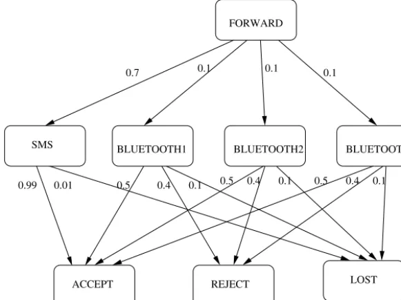
In Section2, we provide a brief review of logical combination methods. In Section3, we introduce the notation that will be used throughout the article. We then present the combined model checking algorithm for the modal case, and establish its completeness and complexity in Section4. In Section5, we extend the combined model checking algorithm to include real-time logics, apply our method to some existing logics, and present some complexity results. Finally, in Section6, we apply the combination method to the Scatterboxmessage-forwarding system to demonstrate the usefulness of our generic model checking approach. We close with a discussion of our results and potential future work in Section7.

2. Combinations of logics

Much work has been carried out on the combination of various modal/temporal logics.Temporalisation,fusion (or inde-pendent combination), andproduct(or join) are among the popular forms of logic combination[27–30].

To provide an overview of these different types of combinations, let us ﬁrst assume that we want to combine two logics, Logic1andLogic2. Further, let us assume thatLogic1is a temporal logic of some form. Let us represent these graphically as

Temporalisation. This is a method that adds a temporal dimension to another logic system. With this method, an arbitrary logic system is combined with temporal modalities to create a new system. Basically a combination of two logics, A and B, resulting in a logic A

(

B

)

, where a pure subformula of B can be treated as an atom within A. Consequently, the combination is notsymmetric— the logic A is the main one, but at each world/state described by A, we might have a formula of B that describes a ‘B-world’.

Temporalisation is investigated in[31], where the logical properties soundness, completeness, and decidability are analysed. In [25] a model checking procedure is presented for temporalised logics. However, the procedure only covers combining modal propositional temporal logics.

(4)

Note that the two logics are essentially independent (hence the name). This means properties such asOPAOPB

ϕ

⇔

OPBOPA

ϕ

, whereOPXis an operator in logic X, are rarely valid. (For tighter linking of this kind we use the product combination below.) The logical properties of fusion, such as soundness, completeness, and decidability, are analysed in [31], while[25]tackles the model checking problem for the fusion of modal temporal logics.

Product (or ‘Join’). In both, temporalisation and independent join, formulas are evaluated at a single node of a model. In contrast to this, the join of two temporal system ﬂows of times are considered over a higher-dimensional plane. Thus, when using the join method, it is possible to produce higher-dimensional temporal logics by combining lower-dimensional temporal logics.

This product combination is similar to fusion, but with a much tighter integration of the logics. The join of two logics A and B is denoted A

⊗

B, and can be visualised as follows.

Speciﬁcally, the operators of the constituent logics tend to be commutative. That is, we have axioms such as

OPAOPB

ϕ

⇔

OPBOPA

ϕ

. The product construction is investigated in[31], where logical properties of soundness, completeness, and decid-ability are analysed. In[25]a combined model checking procedure for modal temporal logic products is presented.

The decision problem for product logics is typically more complex than that for fused logics, with products of relatively benign logics even becoming undecidable. For this reason, product logics are rarely used in practise, with fusions being the main tool for combining logics in a deductive way. However, we argue that this disadvantage does not extend to model checking product logics. This observation turns the model checking problem for products of logics into a feasible approach. We end this section by giving some results for the combining methods mentioned above. Most of the work carried out on combining logics has been from adeducibility or expressivenesspoint of view. To generalise many years of important research, we can say that, usually, decidability and axiomatisability properties transfer to both temporalisations and fusions from the constituent logics [32,33]. Thus, the fusion of two decidable ‘normal polyadic polymodal logics’ is decidable[34]. Work in [35] obtained decidability for modal logics with the ‘converse operator interpreted over transitive frames’. The temporalisation and fusion of the one-dimensional logic PLTL, i.e., PLTL(PLTL) and PLTL

⊕

PLTL, respectively, are also found to be decidable [31,27]. In the case of join, the combinations are less tame: S5

⊗

S5 is NEXPTIME-complete [36], S53 is undecidable[37], and PLTL

⊗

PLTL is undecidable[38], too.

3. Preliminaries

In this section, we deﬁne the notation that will be used throughout the article. The logics we will deﬁne are mainly branching logics, because most of the examples we will discuss later are based on branching-time temporal logics.

3.1. Computation tree logic (CTL)

CTL is a branching-time temporal logic with a discrete notion of time and only future modalities. The temporal operators of CTL allow us to express properties aboutsomeorallcomputations. CTL is deﬁned according to the following grammar:

ϕ

::=

true

|

p

| ¬

ϕ

|

ϕ

1

∧

ϕ

2

| ∃

ψ

| ∀

ψ

(5)

wherep

∈

AP, which is a set of atomic propositions. CTL formulas are interpreted over transition systems, which are a class ofKripke structures. The execution of a transition system constructs a set ofpaths, which are inﬁnite sequences of states. The ith element of a path

σ

is denoted by

σ

[

i

]

. The set of paths from a statesis denoted byPaths

(

s

)

.

Deﬁnition 3.1. Assume

M

=

S

,

E

,

l

is a transition system, where S is a ﬁnite set of states,

E

is a transition relation and S

→

2AP is a labelling function. For a given CTL-formula

ϕ

and state s

∈

S, the satisfaction relation

|

is inductively deﬁned on the structure of

ϕ

as follows:

M

,

s

|

p iff p

∈

l

(

s

)

M

,

s

| ¬

ϕ

iff

M

,

s

|

ϕ

M

,

s

|

ϕ

1

∧

ψ

2 iff

M

,

s

|

ϕ

1and

M

,

s

|

ϕ

2

M

,

s

| ∃

ψ

iff

M

,

σ

|

ψ

for some

σ

∈

Paths

(

s

)

M

,

s

| ∀

ψ

iff

M

,

σ

|

ψ

for all

σ

∈

Paths

(

s

)

Path formulas are deﬁned on the following semantics:

M

,

σ

|

ϕ

iff

M

,

σ

[

1

] |

ϕ

M

,

σ

|

ϕ

1

U

ϕ

2 iff

∃

i

0 s.t.

M

,

σ

[

i

] |

ϕ

2and

(

∀

j

<

i

)

M

,

σ

[

j

] |

ϕ

1

3.2. Probabilistic CTL (PCTL)

PCTL[39]is an extension of CTL, which can express statements such as “the probability that a process eventually termi-nates is 0.2”, “the probability that the system energy exceeds a certain value is

0

.

8”, etc. PCTL is interpreted over (Markov chainsor)Markov decision processes.

Deﬁnition 3.2.AMarkov decision processis a tuple

S

,

A

,

E

,

μ

,

l

, where

– Sis a ﬁnite set ofstates; – A is a ﬁnite set ofactions;

–

E

⊆

S

×

A

×

S is a ﬁnite set ofedges;

–

μ

:

E

→ [

0

,

1

]

is aprobability transition function,1 such that, for all s

∈

S anda

∈

A,

_e_∈_Ea

s

μ

(

e

)

=

1, where

E

a s denotes

the edges fromswith the actiona chosen, i.e.,

E

a_s

= {

s

,

a

,

s

∈

E

}

; – l

:

S

→

2AP _{is a labelling function.}

The execution of a Markov decision process (MDP) constructs a set of paths, which are inﬁnite sequences of states. A probability measure

π

mfor a set of paths with a common preﬁx of the lengthn,s0

→

s1

→ · · · →

sn, is deﬁned to be the

product of transition probabilities along the preﬁx, i.e.,

μ

(

s0,a1,s1

)

× · · · ×

μ

(

sn−1,an

,

sn

)

[39].

Apart from the usual operators from classical logic such as

∧

(and),

∨

(or) and

⇒

(implies), PCTL has theprobabilistic operatorP_∼r, where 0

r

1 is aprobability boundand

∼∈ {

<, >,

,

=}

. Intuitively, a statesof a model satisﬁes P∼r

[

ϕ

]

if, and only if, the probability of taking a path froms that satisﬁes thepath formula

ϕ

is bounded by ‘

∼

r’. The following path formulas

ϕ

are allowed:

ϕ

,

ϕ

U

ψ

and

ϕ

U

k

_ψ

_(where_k

_∈

_N

_{). The semantics of PCTL formulas is given below:}

Deﬁnition 3.3.Assume

M

=

S

,

A

,

E

,

μ

,

l

is a Markov decision process. For a given PCTL-formula

ϕ

and a states

∈

S, the satisfaction relation

|

ϕ

as follows[39]:

M

,

s

|

p iff p

∈

l

(

s

)

M

,

s

| ¬

ϕ

iff

M

,

s

|

ϕ

M

,

s

|

ϕ

1

∧

ϕ

2 iff

M

,

s

|

ϕ

1and

M

,

s

|

ϕ

2

M

,

s

|

P_∼r

[

ψ

]

iff

π

m

σ

∈

Paths

(

s

)

s.t.

M

,

σ

|

ψ

∼

r

Path formulas are deﬁned on the following semantics:

1 _{In order to keep the syntax simple, we consider only one probability distribution}_{μ. It is straightforward to modify our deﬁnition to accommodate a}

(6)

M

,

σ

|

ϕ

iff

M

,

σ

[

1

] |

ϕ

M

,

σ

|

ϕ

1

U

ϕ

2 iff

∃

i

0 s.t.

M

,

σ

[

i

] |

ϕ

2and

(

∀

j

<

i

)

M

,

σ

[

j

] |

ϕ

1

M

,

σ

|

ϕ

1

U

k

ϕ

2 iff

∃

i

ks.t.

M

,

σ

[

i

] |

ϕ

2and

(

∀

j

<

i

)

M

,

σ

[

j

] |

ϕ

1

As an example, the property that “the probability of

ϕ

eventually occurring is greater than or equal to b” can be ex-pressed in PCTL as follows:

Pb

[

true

U

ϕ

]

.

3.3. Timed automata

A timed automaton [40] is a transition system with a ﬁnite set of real-valued clocks. As time progresses, all clocks increase their values at the same rate. In each transition, some clocks can be reset, and the remaining clocks continue to proceed their values. Therefore, clock values denote the elapse of time units since the last reset of the clocks. In a timed automaton, transitions are associated with clock constraints, which are calledguards(enabling conditions). A transition is enabled if the corresponding guard is satisﬁed by the current clock values. Assume C is a set of clocks. The set of clock constraints over C, denoted by

Ψ (

C

)

, is deﬁned by the following syntax:

ψ

::=

true

|

x

∼

k

| ¬

ψ

|

ψ

1

∧

ψ

2

where x

∈

C, k

∈

N

and

∼∈ {

<, >,

,

=}

. When a transition is enabled, a set of clocks are reset to zero, while the remaining clocks keep their values. In addition to clock constraints enabling transitions, timed automata might also contain clock constraints that are used to restrict the time spent in locations. Such constraints are called invariances. They are deﬁned in a similar way to guards.

Deﬁnition 3.4.(See[40].) Atimed automaton

A

is a tuple

L

,

A

,

C

,

E

,

inv

,

l

, where

– Lis a finite set of locations; – Ais a finite set of actions; – C is a finite set of clocks;

–

E

⊆

L

×

Ψ (

C

)

×

A

×

2C

×

Lis a set of edges between locations;

– inv

:

L

→

Ψ (

C

)

is a function associating each location with some clock constraint in

Ψ (

C

)

; – l

:

L

→

2AP is a labelling function (APis a set of atomic propositions).

In the deﬁnition above, the invariance functioninvassigns clock constraints to locations. The automaton might stay in a location

whileinv

()

holds. As soon asinv

()

becomes false, the automaton makes a transition, such that the current clock values satisfy the clock constraints (guard) of this transition. Let

,

∈

Lbe two locations,

γ

∈

Ψ (

C

)

be a clock constraint, a

∈

A be an action, and X

⊆

C be a set of clocks. Anedge (transition) is denoted by a tuple

,

γ

,

a

,

X

,

, which can be informally interpreted as “the automaton moves from

to

if the current clock values satisfy the clock constraint

γ

; if this is the case, the actionais taken and all the clocks of X are reset to zero”.

Here, we define the semantics of timed automata. To do this, we first introduce further notation. Clock constraints are defined on clock valuations. Aclock valuation

ν

over a clock setC is a mapping fromC to

R

0, i.e.,

ν

:

C

→

R

0. The value of a clockx

∈

C is denoted by

ν

(

x

)

. The set of all clock valuations ofC is denoted by

R

C

0. Let

ν

∈

R

C0 be a clock valuation andd

∈

R

₊be a positive real number.

ν

+

ddenotes the clock valuation which assigns each clockx

∈

Cto the value

ν

(

x

)

+

d.

ν

[

x

]

denotes the clock valuation which resetsxto 0, and keeps the values of other clocks same. Also, we write

ν

|

x

∼

kif, and only if,

ν

satisﬁesx

∼

k, i.e.,

ν

(

x

)

∼

k.

We can deﬁne the semantics of a timed automaton in terms of atimed transition system:

Deﬁnition 3.5.(See[41].) Atimed transition system

T

_Aof a timed automaton

A

=

L

,

A

,

C

,

E

,

inv

,

l

is a tuple

S

,

A_T

,

→

,

l_T

, where

– S

= {

,

ν

|

∈

L

,

ν

∈

R

C

0 s.t.

ν

|

inv

()

}

, – A_T

=

A

∪

R

₊,

–

→ ⊆

S

× {

A

∪

R

+} ×Scan be deﬁned in either of the rules below:

–

,

ν

→

d

,

ν

+

d

iff

∃

d

∈

R

₊ s.t.

ν

+

d

|

inv

()

,

∀

(

0

d

)

, –

,

ν

→

a

,

ν

iff

,

γ

,

a

,

X

,

∈

E

,

ν

|

γ

,

ν

=

ν

[

X

]

and

ν

|

inv

(

)

, – l_T

(

,

ν

)

=

l

()

∪ {

γ

∈

Ψ (

C

)

|

ν

|

γ

}

.

(7)

a possible behaviour of the automaton

A

, and it is deﬁned as an inﬁnite sequences0 ξ0

→

s1

ξ1

→

s2

ξ2

→ · · ·

, where

ξ

i

∈

A

∪

R

+ (for i

∈

N

). The ith element of a path is denoted by

σ

[

i

]

. The set of all paths from a state s is denoted by Paths

(

s

)

. The elapsed time of reaching a statesfrom a stateswithin a path

σ

is the sum of the delays along the path, and it is denoted as

T

(

s

→

σ s

)

.

As mentioned above,

T

_A has an infinite number of states. However, some of the states do not differ for some clock valuations in the sense that they display a similar behaviour modulo bisimulation. We therefore define the notion ofclock equivalence, which is used to obtain a finite region graph.

Letintegraland fractional parts of d

∈

R

₊ be denoted by

d

and frac

(

d

)

, respectively, and cx be the largest constant

forx

∈

C that is compared in some clock constraint in

A

or in a formula

ϕ

. (Clock constraints might also exist in logical formulas, cf. Section 3.4.) Given two clock valuations

ν

and

ν

,

ν

isequivalent to

ν

, denoted

ν

∼

=

ν

, if, and only if, the following is true[40]:

–

∀

x

∈

C,

ν

(

x

) >

cx iff

ν

(

x

) >

cx and

–

∀

x

,

y

∈

C,

ν

(

x

)

cx and

ν

(

y

)

cy implies

–

ν

(

x

)

=

ν

(

x

)

,

– frac

(

ν

(

x

))

=

0 ifffrac

(

ν

(

x

))

=

0, and

– frac

(

ν

(

x

))

frac

(

ν

(

y

))

ifffrac

(

ν

(

x

))

frac

(

ν

(

y

))

.

Let

∼

₌

be a clock equivalence on C. For any

γ

∈

Ψ (

C

)

,

ν

∼

=

ν

implies that

ν

|

γ

iff

ν

|

γ

[40]. The equivalence class of

ν

∈

R

C

0, which is denoted by

[

ν

]

, is deﬁned by

[

ν

] = {

ν

∈

R

C0

|

ν

∼

=

ν

}

. Since the set of equivalence classes is finite, this allows us to define a finite region graph.

Deﬁnition 3.6. (See[41].) Given a timed automaton

A

=

L

,

A

,

C

,

E

,

inv

,

l

, theregion transition system

R

(

A

)

of the automa-ton

A

is a tuple

Qr

,

Ar

,

Er

,

lr

, where

– Qr

= {

,

[

ν

] |

∈

L

,

ν

∈

R

C0

}

, – Ar

=

A

∪ {

λ

}

,

–

Er

is deﬁned by as follows:

–

,

[

ν

]

, λ,

,

succ

(

[

ν

]

)

∈

Er

iffsucc

(

[

ν

]

)

|

inv

()

,

–

,

[

ν

]

,

a

,

[

ν

] ∈

Er

iff

,

γ

,

a

,

X

,

∈

E

,

ν

|

γ

,

ν

=

ν

[

X

]

and

ν

|

inv

(

)

, – lr

(

,

[

ν

]

)

=

l

()

∪ {

γ

∈

Ψ (

C

)

|

ν

|

γ

}

wheresucc

(

[

ν

]

)

is the successor equivalence class, deﬁned as follows [40]: Let

α

and

β

be a two equivalence classes such that

α

=

β

. We saysucc

(

α

)

=

β

iff for every

η

∈

α

, there existst

∈

R>

0such that for allt

<

t,

η

+

t

∈

β

and

η

+

t

∈

α

∪

β

.

Deﬁnition 3.6suggests that the region transition system is constructed by considering timed regions as states. As seen in the deﬁnition of

Er

, we label all timed transitions with a special symbol

λ

to represent a time step. We also extend the labelling functionlrwith the atomic clock constraints of

A

that are true at each location.

3.4. Timed CTL (TCTL)

TCTL[40]is a real-time extension of the branching time logic CTL, where constraints on duration are added to temporal operators. It is a logic, in which timing properties of complex systems can be expressed, something which cannot be done using classical temporal logics. Given that

∼∈ {

<, >,

,

=}

,c

∈

N

andp

∈

AP, TCTL is deﬁned according to the following syntax:

ϕ

::=

true

|

p

| ¬

ϕ

|

ϕ

1

∧

ϕ

2

| ∃

ϕ

1

U

∼c

ϕ

2

| ∀

ϕ

1

U

∼c

ϕ

2

The operators

♦

∼c _and

₂

∼c_{can be derived in usual way. These operators are extensions of the standard}

_♦

_and

₂

_operators

with timing constraints. For example, the formula

∃♦

5 on states that “the system will be in the onstate within 5 time units”.

TCTL can be used to express properties of timed automata. Its formulas are interpreted over a timed transition system. Below we deﬁne the semantics:

Deﬁnition 3.7.Assume

A

=

L

,

A

,

C

,

E

,

inv

,

l

is a timed automaton, and

T

_A

=

S

,

A_T

,

→

,

l_T

is the corresponding timed transition system of

A

. For a given TCTL-formula

ϕ

and a states

=

,

ν

in

T

_A, the satisfaction relation

|

ϕ

as follows:

(8)

T

A

,

s

|

ϕ

1

∧

ϕ

2 iff

T

A

,

s

|

ϕ

1and

T

A

,

s

|

ϕ

2

T

A

,

s

| ∃

ϕ

1

U

∼c

ϕ

2 iff

∃

σ

∈

Paths

(

s

)

withs

=

σ

[

0

]

and

∃

i

0s

=

σ

[

i

]

s.t.

T

s

→

σ s

∼

c

,

T

_A

,

s

|

ϕ

2and

∀

j

<

iwiths

=

σ

[

j

]

T

_A

,

s

|

ϕ

1

T

A

,

s

| ∀

ϕ

1

U

∼c

ϕ

2 iff

∀

σ

∈

Paths

(

s

)

withs

=

σ

[

0

]

and

∃

i

0s

=

σ

[

i

]

s.t.

T

s

→

σ s

∼

c

,

T

_A

,

s

|

ϕ

2and

∀

j

<

iwiths

=

σ

[

j

]

T

_A

,

s

|

ϕ

1

We say that

A

|

ϕ

iff

T

_A

,

ν

0

|

ϕ

, where

,

ν

0

∈

S is the initial state[40].

3.5. Probabilistic timed automata

Probabilistic timed automata are an extension of timed automata with discrete probability distributions, or an extension of Markov decision processes with clocks[42]. They are used to model systems that exhibit probabilistic behaviour, such as communication protocols, physical sensors, complex network systems, etc. Probabilistic timed automata are different from timed automata in the sense that transitions between locations can bebothnon-deterministic and probabilistic. In addition to the time aspect existing in timed automata, probabilistic timed automata provide a probability distribution to make a probabilistic choice among the set of enabled edges[43].

Below we give a deﬁnition of probabilistic timed automata, slightly different to that of[43] in the sense that we add actions providing a probabilistic distribution over transitions. Therefore, our deﬁnition of probabilistic timed automata is more general and more expressive, because we extend timed automata with actions, which is not the case in[43].

Deﬁnition 3.8.Aprobabilistic timed automaton(PTA) is a tuple

L

,

A

,

C

,

E

,

inv

,

μ

,

l

, where

– Lis a finite set of locations; – Ais a finite set of actions; – C is a finite set of clocks;

–

E

⊆

L

×

Ψ (

C

)

×

A

×

2C

×

Lis a set of edges between locations;

– inv

:

L

→

Ψ (

C

)

is a function associating each location with some clock constraints in

Ψ (

C

)

; –

μ

:

E

→ [

0

,

1

]

is aprobability transition function,2_{s.t., for all}

_∈

_L_and_a

_∈

_A

e∈Ea

μ

(

e

)

=

1 where

E

adenotes the edges

from

with the actionais chosen, i.e.,

E

a

= {

,

γ

,

a

,

X

,

∈

E

}

; – l

:

L

→

2AP _{is a labelling function (AP}_{is a set of atomic propositions).}

The semantics of probabilistic timed automata is deﬁned in terms of aprobabilistic timed transition system. All the nota-tions deﬁned in Section3.3are also used for PTAs.

Deﬁnition 3.9. Aprobabilistic timed transition system

P

_Aof the probabilistic timed automaton

A

=

L

,

A

,

C

,

E

,

inv

,

μ

,

l

is a continuous time Markov decision process

S

,

A_T

,

→

,

l_T

, where

– S

= {

,

ν

|

∈

L

,

ν

∈

R

C

0 s.t.

ν

|

inv

()

}

, – A_T

= {

a

,

μ

|

a

∈

A

} ∪

R

₊,

–

→⊆

S

×

A_T

×

S can be deﬁned in either of the rules below:

–

,

ν

→

d

,

ν

+

d

iff

∃

d

∈

R

₊ s.t.

ν

+

d

|

inv

()

,

∀

(

0

d

)

,

–

,

ν

a,

→

μ

,

ν

iffe

=

,

γ

,

a

,

X

,

∈

E

,

μ

(

e

) >

0,

ν

|

γ

,

ν

=

ν

[

X

]

and

ν

|

inv

(

)

, – l_T

(

,

ν

)

=

l

()

∪ {

γ

∈

Ψ (

C

)

|

ν

|

γ

}

.

Each path of

P

_Acorresponds to a possible behaviour of

A

, and it is deﬁned as an inﬁnite sequences0 ξ0

→

s1

ξ1

→

s2

ξ2

→ · · ·

, where

ξ

i

∈ {

a

,

μ

|

a

∈

A

} ∪

R

+ (i

∈

N

). Executions of

A

can be obtained by resolving both non-deterministic and proba-bilistic choices, which can be achieved usingschedulers. This process is not the subject of this article, so we refer the reader to[43]for a detailed discussion.

We now deﬁne a ﬁnite-stateregion transition systemas in Section3.3. The idea of constructing region graphs for proba-bilistic timed automata is very similar to that of timed automata. However, in the probaproba-bilistic case, the region graphs are in the form of Markov decision processes[43]. We transfer the concepts and properties introduced for the construction of region graphs for timed automata.

2 _{In order to keep the syntax simple, we consider only one probability distribution}_{μ. It is straightforward to modify our deﬁnition to accommodate a}

(9)

Deﬁnition 3.10. Given a probabilistic timed automaton

A

=

L

,

A

,

C

,

E

,

inv

,

μ

,

l

, theregion transition system

R

(

A

)

of the automaton

A

is a tuple

Qr

,

Ar

,

Er

,

μ

r

,

lr

, where

– Qr

= {

,

[

ν

] |

∈

L

,

ν

∈

R

C0

}

, – Ar

=

A

∪ {

λ

}

,

–

Er

is deﬁned as follows:

–

,

[

ν

]

, λ,

,

succ

(

[

ν

]

)

∈

Er

iffsucc

(

[

ν

]

)

|

inv

()

,

–

,

[

ν

]

,

a

,

[

ν

] ∈

Er

iff

,

γ

,

a

,

X

,

∈

E

,

ν

|

γ

,

ν

=

ν

[

X

]

and

ν

|

inv

(

)

, – for everyer

∈

,

[

ν

]

,

α

,

[

ν

] ∈

Er

μ

r

(

er

)

=

1 if

α

=

λ

e∈Adms(,ν,a,,ν)μ(e)

e∈Adms(,ν,a)μ(e) if

α

=

a

– lr

(

,

[

ν

]

)

=

l

()

∪ {

γ

∈

Ψ (

C

)

|

ν

|

γ

}

,

where

Adms

(

,

ν

,

a

)

= {

,

γ

,

a

,

X

,

¯

∈

E

|

ν

|

γ

and

ν

[

X

] |

inv

(

)

¯

}

Adms

(

,

ν

,

a

,

ν

)

= {

,

γ

,

a

,

X

,

∈

E

|

ν

|

γ

,

ν

=

ν

[

X

]

and

ν

|

inv

(

)

}

[44].

Informally speaking, Adms

(

,

ν

,

a

)

is the set of all admissible edges from the location

by executing the action a, and Adms

(

,

ν

,

a

,

ν

)

is the set of all admissible edges from

to

through executing a. Note that the deﬁnitions Adms

(

,

ν

,

a

)

and Adms

(

,

ν

,

a

,

ν

)

mark different sets. The former considers the edges to all target locations which are reached by resetting some clocks; the latter considers the edges to the target location

which is reached by executing the actionaand resetting some clock set. So, the latter is a subset of the former.

As in Section 3.3, we label all timed transitions with a special symbol

λ

representing time steps. We also extend the labelling functionlrwith the atomic clock constraints of

A

which are true at each location.

4. Generic model checking for modal, temporal, and probabilistic logics

In this section, we generalise the model checking algorithm for combined logics given in[25] to cover more complex cases, such as knowledge,belief, andprobability. As we have seen in the previous section, the semantics of these logics is deﬁned over more general structures than standard Kripke structures. In our extended model checking algorithm, different model types of combined logics are therefore assumed to have an appropriate hybrid model type.

In the sequel, the following general deﬁnition can be used for a propositional logic. (We assume a propositional extension of modal logic.) The language is built from a countable signature of propositional letters AP

= {

p1,p2, . . .

}

, the boolean connectives

∧

and

¬

, a set of operatorsOP

= {

Oi1

1

, . . . ,

O in

n

}

with aritiesi1, . . . ,in (forn

∈

N

), respectively, and the following

formation rules:

– every propositional letter p

∈

APis a formula; – if

ϕ

1,

ϕ

2are formulas, so are

¬

ϕ

1and

ϕ

1

∧

ϕ

2; – if Oik

k

∈

OPand

ϕ

1, . . . ,

ϕ

ik are formulas, so areO ik

k

(

ϕ

1, . . . ,

ϕ

ik

)

(fork

∈

N

).

The other boolean connectives, such as

∨

,

→

, and

↔

, and the constants

⊥

and

can be deﬁned as usual. Depending on the type of the logic, e.g., temporal, probabilistic, belief etc., the semantics is deﬁned over different structures, such asKripke structures,Markov chains,interpreted systems, etc.

In this section, we assume models withexplicitsets of states, such as Kripke structures, with a discrete labelling function. In Section 5, we will discuss the case of models withsymbolic states, such as timed automata. For simplicity, we do not denote initial states in the structure of a model. This can be added without any problem.

Assume a frame is a Kripke structure without a valuation function, i.e., a pair

S

,

T

where S is a non-empty set of states, andT is a relation deﬁned onS. Given that

S1,T1

is a frame for the logic A and

S2,T2

is a frame for the logic B, a model

M

for A

(

B

)

is a tuple

S1

∪

S2,T1,T2,l

. Note thatT1 (resp.T2) is ann-tuple denoting a relation with an arbitrary (possibly empty) labellingof states andaccessibility relations on states. Since we consider A and B to be any modal logic, we assume thatT can be more general than the accessibility relation, which is usually denoted byR. Namely, T1 (resp.T2) gets a different form according to the type of logic A (resp. B). For example, if A (resp. B) is amodallogic, then T1 (resp. T2) is deﬁned simply as theaccessibility relation R. If, however, A (resp. B) is aprobabilisticlogic, T1 (resp.T2) will be the transition relation with probability labels on edges. In Section4.4 we show how T1 (resp. T2) can have different forms according to the type of the logic. We note that within temporalisation,l

:

S2

→

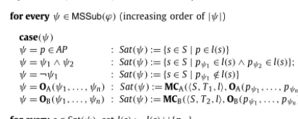
2AP is a labelling function assigning S2 to sets of proposition letters.

(10)

MCAB

Input:M= S,T1,T2,land AB formulaϕ

for everyψ∈MSSub(ϕ)(increasing order of|ψ|)

case(ψ)

ψ=p∈AP :Sat(ψ):= {s∈S|p∈l(s)}

ψ=ψ1∧ψ2 :Sat(ψ):= {s∈S|pψ1∈l(s)∧pψ2∈l(s)}; ψ= ¬ψ1 :Sat(ψ):= {s∈S|pψ1∈/l(s)}

ψ=OA(ψ1, . . . , ψn) : Sat(ψ):=MCA(S,T1,l,OA(pψ1, . . . ,pψn))

ψ=OB(ψ1, . . . , ψn) :Sat(ψ):=MCB(S,T2,l,OB(pψ1, . . . ,pψn))

[image:10.561.168.380.82.167.2]

for everys∈Sat(ψ), setl(s):=l(s)∪ {pψ}

Fig. 1.Model checking algorithmMCABfor the combination of the logics A and B.

The algorithm inFig. 1can be used for model checking the combined logic A(B) with the inputs

M

and

ϕ

. The procedure ﬁrst computes MSSub

(

ϕ

)

, a set of maximal state subformulas of

ϕ

. The maximal state subformulas is the smallest set of subformulas of

ϕ

that satisﬁes the following constraints:

• ϕ

is inMSSub

(

ϕ

)

,

•

if

ψ

is in MSSub

(

ϕ

)

and

ψ

does not start with an operator ofOPAthen the maximal subformulas of

ψ

that do start with anOPA operator is inMSSub

(

ϕ

)

,

•

if

ψ

is inMSSub

(

ϕ

)

and

ψ

does not start with an operator ofOPB then the maximal subformulas of

ψ

that do start with anOPB operator is inMSSub

(

ϕ

)

,

•

the atomic propositions that occur in

ϕ

are inMSSub

(

ϕ

)

,

•

if

ψ

is inMSSub

(

ϕ

)

and

¬

ψ

is a subformula of

ϕ

, then

¬

ψ

is inMSSub

(

ϕ

)

, and

•

if

ψ

and

ψ

are inMSSub

(

ϕ

)

and

ψ

∧

ψ

is a subformula of

ϕ

, then

ψ

∧

ψ

is inMSSub

(

ϕ

)

.

For example, consider the A

(

B

)

formula

∀

(true

U

(

∃♦ ∃

2

p

)

), where OPA

= {∀

,

U

}

andOPB

= {∃

,

♦

,

2 }

. According to the deﬁnition, the maximal state subformulas of A and B are

{∀

U

}

and

{∃♦ ∃

2 ,

p

}

, respectively. Note that

∃

2

is a not a maximal state subformula. The maximal state subformulas of the logic A are designed to keep the number of calls to the component model checkers low.

The procedure then model checks formulas in MSSub

(

ϕ

)

in increasing order of length of subformulas and extends the labelling l within

M

accordingly. The parse tree of

ϕ

is recursively descended. For each maximal state subformula

ψ

of

ϕ

, the satisfaction set Sat

(ψ)

, representing the set of states where

ψ

holds, is calculated. For propositional formulas p

∈

AP, the procedure is trivial. Formulas, whose main operator is in the language of the logics A resp. B are resolved by taking advantage of the corresponding model checker. Prior to calling this model checker, the input to the model checker is modiﬁed: for formulas OA(ψ1, . . . , ψn

)

andOB(ψ1, . . . , ψn

)

, every subformula

ψ

i (for 1

i

n) is replaced by a new

proposition pψi. This is simply because

ψ

i can be either from A or B; therefore we cannot applyMCA toOA(ψ1, . . . , ψn

)

if

a subformula

ψ

i is a B-formula (and vice versa).

Note that the OA(ψ1, . . . , ψn

)

and OB(ψ1, . . . , ψn

)

are not necessarily operators from the component logics; they are

rather formula trees in the component logics. For boolean formulas, e.g.,

ψ

=

ψ1

∧

ψ2

, the satisfaction set of the formula

ψ

is calculated according to the set of states where pψ1 andpψ2 hold.

In Fig. 1, we assume model checkers take a model and a formula

ψ

as input and return the set of states at which

ψ

holds.

4.1. Fusion (independent combination)

Let A and B be two propositional logics. A structure

M

for A

⊕

B is a tuple

S1

∪

S2,T1,T2,l

, where T1 (resp.T2) is a tuple whose elements depend on the type of A (resp. B). Given that

M

is a ﬁnite A

⊕

B-structure and

ϕ

is an A

⊕

B-formula, the model checking problem for A

⊕

B is to check whether there existss

∈

S1

∪

S2 such that

M

,

s

|

A⊕B

ϕ

. The algorithm inFig. 1can again be used for model checking A

⊕

B with the input

M

and

ϕ

.

Remark 1.Note that temporalisation is a special case of fusion.

4.2. Join

(11)

(i) if A (resp. B) is a modal or temporal logic without actions, then given thatT

=

R

=

(

R1

∪

R2),T1

=

R1 (resp.T2

=

R2), whereR1(resp. R2) denotes a binary relation;

(ii) if A (resp. B) is a modal or temporal logic with actions, then given thatT

=

A

=

(

A1

∪

A2),

E

=

(

E

1

∪

E

2)

,T1

=

A1,

E

1

(resp. T2

=

A2,

E

2

), where A1 (resp. A2) is the set of actions for the logic A (resp. B), and

E

1 (resp.

E

2) is the corresponding set of edges for the logic A (resp. B);

(iii) if A (resp. B) is a probabilistic logic, then given that T

=

A

=

(

A1

∪

A2),

E

=

(

E

1

∪

E

2),

μ

, T1

=

A1,

E

1,

μ

1

(resp. T2

=

A2,

E

2,

μ

2

), where

μ

1 (resp.

μ

2) is a probability transition function.

These cases are formally expressed as follows:

case

(

i

)

T1

=

R1

,

where

R1

=

e

=

s1

,

s

,

s1

,

s

∈

Rs.t.s1

=

s1

case

(

ii

)

T1

=

A1

,

E

1

,

where

E

1

=

e

|

e

=

s1

,

s

,

a1

,

s1

,

s

∈

E

s.t.s1

=

s1anda1

∈

A1

case

(

iii

)

T1

=

A1

,

E

1

,

μ

1

,

where

E

1

=

e

=

s1

,

s

,

a1

,

s1

,

s

∈

E

s.t.s1

=

s1anda1

∈

A1

μ

1

(

e

)

=

μ

(

e

)

for everye

∈

E

13

T2 is calculated in a similar way. Given that

M

is a ﬁnite A

⊗

B-structure and

ϕ

is an A

⊗

B-formula, the model checking problem for A

⊗

B is to check whether there exists a

s1,s2

∈

S1

×

S2such that

M

,

s1,s2

|

A⊗B

ϕ

. The algorithm inFig. 1 can again be used for model checking A

⊗

B with inputs

M

and

ϕ

.

Remark 2.Note that we assume we are given a two-dimensional model

S1

×

S2,T

,

l

, from which we calculate the input

M

=

S1

×

S2,T1,T2,l

to the model checker. Therefore, on top of the cost of model checking on

M

, there will be an overhead cost for constructing

M

.

Remark 3. Here we do not consider handshaking (synchronisation) of the action sets A1 and A2. Therefore, we assume A1

∩

A2

= ∅

. We consider the case A1

∩

A2

= ∅

in Section5.2.

4.3. Correctness and complexity

Theorem 4.1(Termination). Let

M

=

S

,

T1,T2,l

be a ﬁnite structure for the combined logicAB. Assume the model checkersMCA andMCBare terminating. Then, the combined model checkerMCABas deﬁned inFig. 1also terminates.

Proof. MCAB computes the set of formulasMSSub

(

ϕ

)

in ﬁnite time. The procedure also extends the labelling functionlthat maps each state to a set of proposition letters in ﬁnite time. Since the model checkersMCA andMCB are also terminating, the combined model checkerMCABterminates.

2

Theorem 4.2(Correctness). Let

M

=

S

,

T1,T2

,

l

be a ﬁnite model for the combination of the logicsAandB, and

ϕ

be a combined formula. Assume the model checkersMCAandMCBare sound, complete and terminating. Then, pϕ

∈

l

(

s

)

if, and only if,

M

,

s

|

AB

ϕ

, where s

∈

S.

Proof. We show by induction over the structure of

ϕ

that, for everys

∈

S that pψ

∈

l

(

s

)

holds if, and only if,

M

,

s

|

AB

ψ

. The base cases,

ψ

=

p(p

∈

AP), is obvious.

For the induction step, the cases of boolean combinations,

ψ

= ¬

ψ1

and

ψ

=

ψ1

∧

ψ2

, of maximal state formulas is trivial. The induction step for the remaining composed modal operators is as follows.

ψ

=

OA(ψ1, . . . , ψn

)

: By induction hypothesis, pψi

∈

l

(

si

)

iff

M

,

si

|

AB

ψ

i holds for all 1

i

n and all si

∈

S. Let

ψ

=

OA(pψ1

, . . . ,

pψn

)

be a formula obtained by replacing the

ψ

i inOA(ψ1, . . . , ψn

)

bypψi.

The soundness and completeness of the model checkerMCAprovides pψ

≡

pOA(ψ1,...,ψn)

∈

l

(

s

)

iff

S1,T1

,

l

,

s

|

A

ψ

. With

S1,T1,l

,

s

|

A

ψ

iff

M

,

s

|

AB

ψ

, we obtainpψ

∈

l

(

s

)

iff

M

,

s

|

AB

ψ

.

ψ

=

OB

(ψ1, . . . , ψ

n

)

: Similar to above case.

2

We now analyse the computational complexity of the model checker MCAB. The complexity of the combined model checker is the sum ofcomponent model checking cost, which is the cost of performing component model checks, and interac-tion processing cost, which is the sum of the cost of processing inputs and outputs of the component model checks and the cost of operations on the labelling function.

3 _{Note that it is trivial to observe that}

e∈Ea

iqμi(e)=1 fori∈ {1,2}(E

a

iqdenotes the edges fromqwith the actionais chosen, i.e.,E

a iq= {q,a,q