Deriving confidence in paleointensity estimates

Q07Z18, doi:10.1029/2010GC003071 ISSN: 1525‐2027

Click Here for

Full Article

Deriving confidence in paleointensity estimates

Greig A. Paterson

National Oceanography Centre, Southampton, University of Southampton, Southampton SO14 3ZH, UK

Now at Paleomagnetism and Geochronology Laboratory, SKL‐LE, Institute of Geology and Geophysics, Chinese Academy of Sciences, Beijing 100029, China ([email protected])

David Heslop

Fachbereich Geowissenschaften, Universität Bremen, Klagenfurter Straße, D‐28359 Bremen, Germany

Adrian R. Muxworthy

Department of Earth Science and Engineering, Imperial College London, South Kensington Campus, London SW7 2AZ, UK

[1] Determining the strength of the ancient geomagnetic field (paleointensity) can be time consuming and

can result in high data rejection rates. The current paleointensity database is therefore dominated by studies that contain only a small number of paleomagnetic samples (n). It is desirable to estimate how many sam-ples are required to obtain a reliable estimate of the true paleointensity and the uncertainty associated with that estimate. Assuming that real paleointensity data are normally distributed, an assumption adopted by most workers when they employ the arithmetic mean and standard deviation to characterize their data, we can use distribution theory to address this question. Our calculations indicate that if we wish to have 95% confidence that an estimated mean falls within a ±10% interval about the true mean, as many as 24 paleomagnetic samples are required. This is an unfeasibly high number for typical paleointensity studies. Given that most paleointensity studies have smalln, this requires that we have adequately defined confi-dence intervals around estimated means. We demonstrate that the estimated standard deviation is a poor method for defining confidence intervals for n < 7. Instead, the standard error should be used to provide a 95% confidence interval, thus facilitating consistent comparison between data sets of different sizes. The estimated standard deviation, however, should retain its role as a data selection criterion because it is a measure of the fidelity of a paleomagnetic recorder. However, to ensure consistent confidence levels, within‐site consistency criteria must be depend onn. Defining such a criterion using the 95% confidence level results in the rejection of∼56% of all currently available paleointensity data entries.

Components: 8900 words, 9 figures, 4 tables. Keywords: paleointensity; error analysis.

Index Terms: 1521 Geomagnetism and Paleomagnetism: Paleointensity; 1594 Geomagnetism and Paleomagnetism: Instruments and techniques; 1599 Geomagnetism and Paleomagnetism: General or miscellaneous.

Received2 February 2010;_Revised4 May 2010;_Accepted20 May 2010;_Published21 July 2010.

Paterson, G. A., D. Heslop, and A. R. Muxworthy (2010), Deriving confidence in paleointensity estimates,Geochem. Geophys. Geosyst.,11, Q07Z18, doi:10.1029/2010GC003071.

Theme: Magnetism From Atomic to Planetary Scales: Physical Principles and Interdisciplinary Applications in Geoscience

Guest Editors: J. Feinberg, F. Florindo, B. Moskowitz, and A. P. Roberts

1. Introduction

[2] Obtaining detailed information about past

geo-magnetic field behavior is key to our understanding of the geodynamo and its evolution. However, obtaining reliable estimates of paleofield strength (paleointensity) is problematic and suffers from high failure rates [e.g., Perrin, 1998; Riisager et al., 2002]. Many studies therefore suffer from having a small number of paleomagnetic samples (Figure 1), which are often insufficient to estimate the uncertainty in the mean result (i.e., n = 1). Currently, >70% of entries in the PINT08 database [Biggin et al., 2009] are from four paleomagnetic samples or less (n ≤4 (Figure 1)). This brings the reliability of paleointensity estimates based on small data sets into question.

[3] If we consider paleointensity data to be

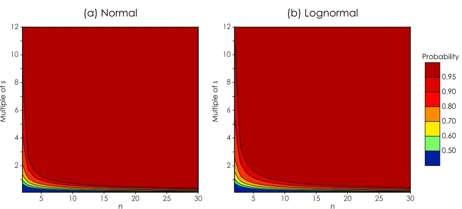
nor-mally distributed, the probability that an estimated mean (m) falls within ±10% of the true mean (m) can be calculated from the normal cumulative dis-tribution function (Figure 2a). If we choose a commonly applied within‐site consistency crite-rion, that the true standard deviation (s) must be

≤25% of the true mean, we can calculate the

number of paleomagnetic samples required for an accurate estimated mean at the 95% confidence level. For the worst case scenario, when = 0.25,

for normally distributed data, n must be ≥24.

Biggin et al. [2003], also assuming normality, estimated the number of paleomagnetic samples

required for 95% confidence that m falls within

±10% of m. Using historical data sets, they esti-mated that at least 6–22 paleomagnetic samples were required to achieve this. Our generally applicable number is larger than the data set

spe-cific values given by Biggin et al. [2003].

Regardless, such large data sets are uncommon in paleointensity studies, therefore confidence limits on estimated means are important for fully quan-tifying paleointensity data.

[4] It is intuitive that sampling small numbers of

point values can lead to fortuitously low, or high, estimated standard deviations (s), and it has been acknowledged in paleointensity studies that a small

standard deviation is no guarantee of accuracy [Biggin et al., 2003]. However, little work has been undertaken to quantify the uncertainties associated with small paleointensity data sets. In this study, we use analytical and numerical calculations to assess the usefulness of statistics commonly used in paleointensity analyses. These calculations are based on the assumption that real paleointensity data are normally or lognormally distributed. These statistics and assumptions will be tested using historical data sets where the true geomagnetic field intensities are known. This is in contrast toBiggin et al.[2003] who used the estimated mean of each data set to define the “true” field intensity.

2. Methods

[5] In statistical theory, a sampling distribution

is the probability distribution of a given statistic obtained from a random selection of point values from a population distribution (the complete dis-tribution of values). When sufficient point values are obtained from a population distribution, the sampling distribution will approximate the popu-lation distribution. Throughout this paper, we use the term sample in the statistical sense of refer-ring to a subset of a population distribution, and refer to physical specimens used in paleointensity studies as paleomagnetic samples. Each individual paleointensity estimate can be viewed as a point value that is randomly selected from a population distribution.

[6] Most paleointensity studies characterize data

using the estimated mean (m) and estimated standard deviation (s) under the assumption of normality, i.e.,

mSxi

n ; ð1Þ

and

s

ffiffiffiffiffiffiffiffiffiffiffiffiffiffiffiffiffiffiffiffiffiffi SðximÞ2

n1 s

wherexiis theith datum andnis the number of data.

Cochran’s theorem tells us that for normally dis-tributed random variables, the distribution of sample (estimated) means and sample (estimated) variances are independent. Sample means follow a normal distribution with true meanm, and true variance_n2, while sample variances are chi‐square (c2) distributed with (n−1) degrees of freedom:

s2¼

2

n1

2

n1: ð3Þ

Hence, sample standard deviations arecdistributed:

s¼ ffiffiffiffiffiffiffiffiffiffiffi n1

p n1: ð4Þ

Examples of the distribution of sample standard deviations are shown in Figure 3.

[7] The known distributions of sample means and

sample variances for normal distributions provides analytical solutions for understanding the behavior of m and s. Details of the analytical solutions are

given in Appendices A–C. Assessing nonnormal

Figure 2. The probability that the estimated mean falls within 10% of the true mean for (a) normally distributed data and (b) lognormally distributed data. The probabilities depend on the true standard deviation (s) of the underlying distribution, which has been scaled as a percentage of the true mean.

Figure 1. Histogram of paleointensity data entries from the PINT08 database [Biggin et al., 2009]. Over 70% of the data entries have n ≤ 4. An additional 71 entries do not reportn.

distributions, however, is more complicated from an analytical view point because the true standard deviation and true mean are frequently dependent, and can be related in a nonlinear fashion. The easiest approach, therefore, is to derive numerical solutions. To assess lognormally distributed data

we have used 106 random samples of varying

size,n, to determine the behavior ofmands. This approach can be generalized for any distribution, as follows.

[8] 1. Randomly select n data from the specified

distribution.

[9] 2. Calculate the estimated mean (m) and

esti-mated standard deviation (s) of thendata, assuming a normal distribution (i.e., equations (3) and (4)).

[10] 3. Repeat the above steps 106 times.

[11] 4. Identify the number of samples that conform

with the criteria to be investigated (e.g., the number of samples with a confidence interval (m± 1s) that includes the true mean). This allows the probability of each outcome to be estimated.

[12] 5. Repeat steps 1–4 for samples of sizen + 1.

[13] The lognormal distribution that we

investi-gated using this approach was set to have a true mean of 30 (a typical geomagnetic field strength in mT) and varying true standard deviations (s = 1%–100% of the true mean). The true standard de-viations are defined as percentages of the true mean, therefore the results are independent of the absolute

value of the true mean. The lognormal distribution parameters (gand) were calculated using standard equations [Aitchison and Brown, 1957]:

True Mean; ¼eþ22; ð5Þ

and

True Standard Deviation; ¼eþ22

ffiffiffiffiffiffiffiffiffiffiffiffiffiffiffiffiffiffi e21

ð Þ q

: ð6Þ

[14] Strictly, the use of equations (1) and (2) in

step 2 is only valid for a normal distribution. How-ever, irrespective of the real paleointensity data distributions, this is how most paleointensity studies analyze their data.

3. Results

3.1. Obtaining an Accurate Estimate of the True Mean

[15] As noted in section 1, n ≥ 24 is required for

95% confidence that mfalls within ±10% of mfor

normally distributed data, under the criterion that= 0.25 (Figure 2a). For lognormally distributed data under the same conditions (Figure 2b), for mto be within ±10% of m,nmust also be≥24 to achieve a 95% confidence level. These two values represent a worst case scenario under these conditions. When is lower, smallerncan be used to achieve the same 95% confidence level.

3.2. Confidence Limits Using the Standard Deviation

[16] To assess the usefulness of the estimated

standard deviation, s, to provide confidence inter-vals for small n, we calculate the probability that the true mean lies within an interval around the estimated mean defined by a multiple of the

esti-mated standard deviation. Strictly, s does not

reflect the precision of m, but rather it represents a coverage interval of the sampling distribution. For normally distributed data the interval m ± 1s will include approximately 68% of the data, and approximately 95% of the data will be included in

the interval m ± 2s. The analytical solution for

normally distributed data and the numerical solution for lognormal data are shown in Figures 4a and 4b, respectively. For the analytical solution, the proba-bilities that m lies within a multiple ofs of m are independent of s. However, for the lognormal dis-tribution these probabilities decrease by∼10% over a two order of magnitude increase ins; the depen-dence onsis most pronounced at lown(<5). This dependence is small enough to be viewed as negli-gible and we have averaged the probabilities over all

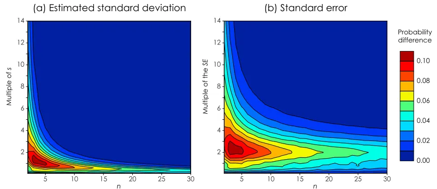
svalues. A contour plot of the maximum probability difference between different values ofs is given in Appendix B.

[17] As would be expected, asnincreases there is a

greater probability of the true mean lying within

±1s. When n = 7 or 8, one estimated standard

deviation is sufficient to provide an uncertainty interval that corresponds to a 95% confidence

interval for normally and lognormally distributed data, respectively. These are more achievable sample numbers for typical paleointensity studies.

When we consider smaller values of n, increasing

multiples ofsare required to provide the same level

of confidence. For n = 2 as many as 8 estimated

standard deviations are needed to define the equivalent 95% confidence interval around the estimated mean for normally distributed data (Figure 4a). Eleven estimated standard deviations are required for lognormally distributed data when n = 2 (Figure 4b).

3.3. Confidence Limits Using the Standard Error

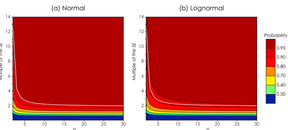
[18] An alternative parameter that can be used to

define the confidence interval around an estimated mean is the standard error (SE), which is defined as

sffiffi n

p . The SE, which is also known as the standard

on s. This dependence produces a maximum probability difference of∼10% and, as above, the probabilities have been averaged over allsvalues

(see Appendix B). In many respects the SE

pro-vides a poorer method of defining confidence intervals around m. The probabilities of mfalling

within a multiple of the SE of m are generally

lower than if s were used, and the confidence

levels defined by the SE are dependent on n.

However, the SE can be used to provide a

con-sistent confidence interval (CI) given that, for a normal distribution, the percentiles of the distribu-tion can be approximated by a t distribution:

CI¼ t1

2;n1

ð Þ s ffiffiffi n

p ¼ t₁

2;n1

ð Þ SE; ð7Þ

where t ₁

2;n1

ð Þ is the two‐tail criticalt value for

the (1 − a) × 100th percentile (i.e., the (1 − a) confidence level) and for (n − 1) degrees of free-dom. The white lines in Figure 5 are the t critical values for nat the 95% confidence level. For nor-mally distributed data, for all n these multiples of the SEprovide 95% confidence that mfalls within

the confidence interval of m. For the lognormal

data, t × SE fails to provide a consistent 95%

confidence level. However, the confidence levels

vary from 91%–94%, with an average of 93%,

which is more consistent than provided by ±1s. In general, the larger the deviation from normality, the lower this confidence level becomes.

3.4. Within‐Site Consistency

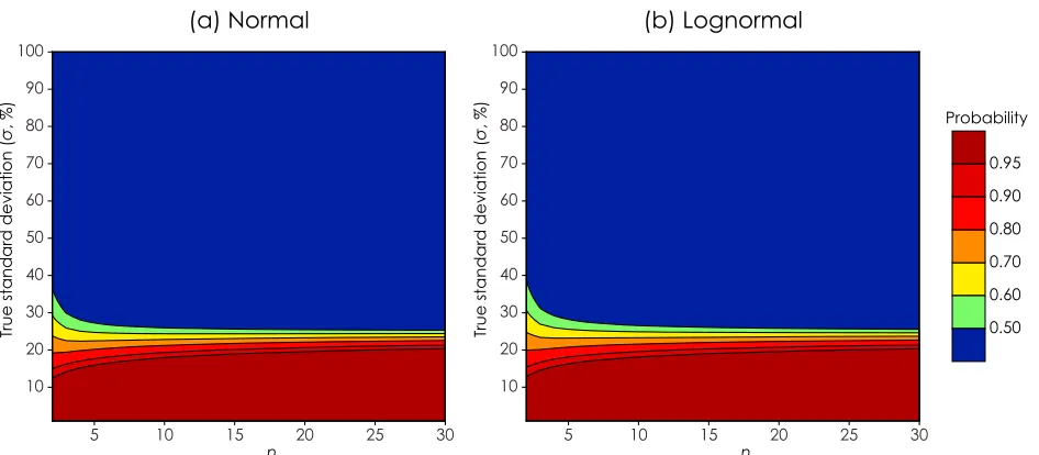
[19] As noted in section 1, low within‐site scatter,

defined as the ratio of the estimated standard

devi-ation to the estimated mean (dB (%) = s

m × 100),

may not be an indication of accuracy and may arise fortuitously when n is small [Biggin et al., 2003]. We calculate the probability thatdB (%)≤25% for randomly sampled data (Figure 6). The probability intuitively has a strong dependence on the true standard deviation of the underlying distribution.

However, the confidence level varies withn. For

n = 2, when the is 15% there is only a ∼90%

probability that dB (%) will be ≤25%, which

increases to >95% for n ≥ 4. Confidence levels are lower for lognormally distributed data, and under

the same circumstances n ≥ 5 is needed for 95%

confidence or better.

4. Discussion

[20] When dealing with real paleointensity data

parameters such as m, s and the SE can be

esti-mated from the data. Only in recent times, with the use of DGRF data [Maus et al., 2005], can we

obtain values for m, but values for s remain

unobtainable. In the following discussion we will look at historical data sets wheremcan be obtained from DGRF data and make use of the criteria outlined above.

4.1. How Are Real Data Distributed? [21] A key issue is how well the considered

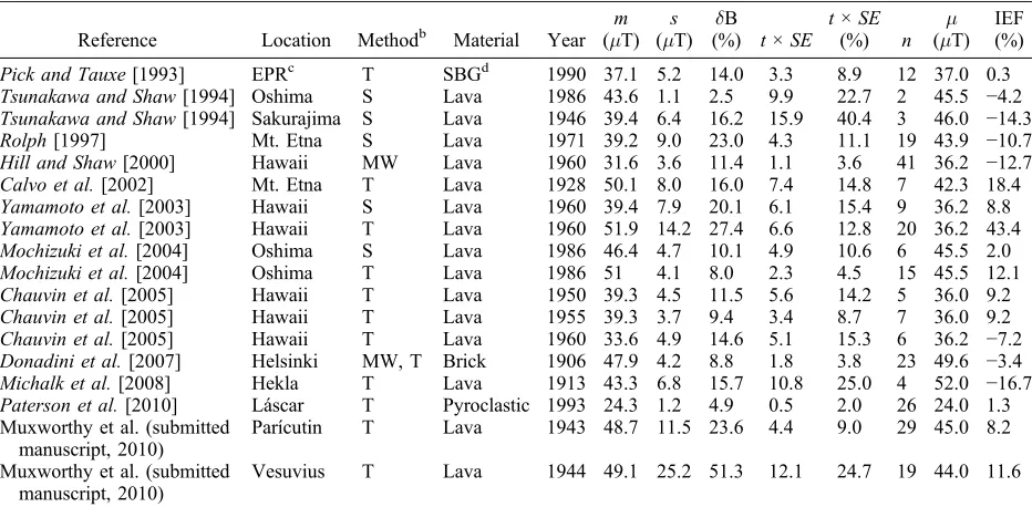
methods and materials are summarized in Table 1. Biggin et al. [2003] used the Anderson‐Darling

(AD) test [Anderson and Darling, 1952;Stephens,

1986] to show that three historical data sets could not be distinguished from a normal distribution at the 0.05 significance level. We expand on this approach by considering additional data sets and testing for lognormality (Table 2). In addition, we have used the AD test to calculate the probability that the data sets are normally distributed withm=m, or that they are lognormally distributed withg= lnm

(which assumes that the true mean is the median value of the lognormal distribution, which greatly simplifies calculations forgand).

[22] For all but one data set (the Parícutin data set

of A. R. Muxworthy et al. (A Preisach methodology to determining absolute paleointensities: 2. Field

testing, submitted to Journal of Geophysical

Research, 2010)) the AD test cannot reject the null hypothesis that the data sets have been sampled from continuous lognormal distributions at the 0.05 significance level. With the exception of four data sets (Pick and Tauxe[1993], the Thellier data from Yamamoto et al. [2003], and both data sets from Muxworthy et al. (submitted manuscript, 2010)),

all data sets could also be sampled from contin-uous normal distributions. Considering the prob-abilities that the data sets are distributed around the expected values (P* values in Table 2), we

observe that the data from Hill and Shaw [2000],

and the Thellier data fromYamamoto et al.[2003] and Mochizuki et al. [2004] are not normally or lognormally distributed. Two of these data sets are from the 1960 lava flow on Hawaii, which has been noted for yielding absolute paleointensity results that are inconsistent with the expected value

[Tanaka and Kono, 1991; Tsunakawa and Shaw,

1994; Hill and Shaw, 2000; Yamamoto et al.,

2003]. This may be the result of bias due to the presence of chemical or thermochemical remanent

magnetizations [e.g., Tsunakawa and Shaw, 1994;

Hill and Shaw, 2000; Yamamoto, 2006; Fabian,

2009]. Mochizuki et al. [2004] noted that their

Thellier data are systematically higher than expected and suggested that an inherent rock magnetic prop-erty or thermal alteration due to laboratory heating has caused this bias.

[23] It is worth considering the statistical power of

the AD test with respect to the data being analyzed. In general, goodness‐of‐fit tests lose accuracy with Table 1. Descriptive Statistics of Real Paleointensity Data Setsa

Reference Location Methodb Material Year m (mT)

s (mT)

dB

(%) t×SE t×SE

(%) n

m (mT)

IEF (%)

Pick and Tauxe[1993] EPRc T SBGd 1990 37.1 5.2 14.0 3.3 8.9 12 37.0 0.3

Tsunakawa and Shaw[1994] Oshima S Lava 1986 43.6 1.1 2.5 9.9 22.7 2 45.5 −4.2

Tsunakawa and Shaw[1994] Sakurajima S Lava 1946 39.4 6.4 16.2 15.9 40.4 3 46.0 −14.3

Rolph[1997] Mt. Etna S Lava 1971 39.2 9.0 23.0 4.3 11.1 19 43.9 −10.7

Hill and Shaw[2000] Hawaii MW Lava 1960 31.6 3.6 11.4 1.1 3.6 41 36.2 −12.7

Calvo et al.[2002] Mt. Etna T Lava 1928 50.1 8.0 16.0 7.4 14.8 7 42.3 18.4

Yamamoto et al.[2003] Hawaii S Lava 1960 39.4 7.9 20.1 6.1 15.4 9 36.2 8.8

Yamamoto et al.[2003] Hawaii T Lava 1960 51.9 14.2 27.4 6.6 12.8 20 36.2 43.4

Mochizuki et al.[2004] Oshima S Lava 1986 46.4 4.7 10.1 4.9 10.6 6 45.5 2.0

Mochizuki et al.[2004] Oshima T Lava 1986 51 4.1 8.0 2.3 4.5 15 45.5 12.1

Chauvin et al.[2005] Hawaii T Lava 1950 39.3 4.5 11.5 5.6 14.2 5 36.0 9.2

Chauvin et al.[2005] Hawaii T Lava 1955 39.3 3.7 9.4 3.4 8.7 7 36.0 9.2

Chauvin et al.[2005] Hawaii T Lava 1960 33.6 4.9 14.6 5.1 15.3 6 36.2 −7.2

Donadini et al.[2007] Helsinki MW, T Brick 1906 47.9 4.2 8.8 1.8 3.8 23 49.6 −3.4

Michalk et al.[2008] Hekla T Lava 1913 43.3 6.8 15.7 10.8 25.0 4 52.0 −16.7

Paterson et al.[2010] Láscar T Pyroclastic 1993 24.3 1.2 4.9 0.5 2.0 26 24.0 1.3

Muxworthy et al. (submitted manuscript, 2010)

Parícutin T Lava 1943 48.7 11.5 23.6 4.4 9.0 29 45.0 8.2

Muxworthy et al. (submitted manuscript, 2010)

Vesuvius T Lava 1944 49.1 25.2 51.3 12.1 24.7 19 44.0 11.6

a

The estimated mean geomagnetic field intensity and estimated standard deviation aremands, respectively;dB (%) =s

m× 100;t×SEis the 95%

confidence interval defined by the standard error and as a percentage of the estimated mean;nis the number of paleomagnetic samples accepted for the mean paleointensity estimate;mis the expected geomagnetic field intensity determined from DGRF data [Maus et al., 2005]; and IEF (%) is the intensity error fraction (=m× 100).

b_{T, data obtained using the Thellier method and its variants [Thellier and Thellier, 1959;Coe, 1967]; S, data obtained using the Shaw method}

and its variants [Shaw, 1974]; MW, data obtained using the microwave method and its variants [Walton et al., 1993].

c_{East Pacific Rise.} d

decreasing n. The AD test is no exception. Given the small size of some of the data sets here, some of the probability should be viewed with caution.

P values (Table 2) were calculated using the

asymptotically derived analytical solution for the AD test [Stephens, 1986]. However, no analytical solution is currently available for theP* probabili-ties, which were therefore estimated using a Monte

Carlo approximation with 107 simulations [e.g.,

Stephens, 1974, 1979]. The effect is that the P* probabilities are poorly constrained close to the tails

of the distribution (i.e., P*≈0.05 and P*≈0.95).

This is of most concern for us when P* ≈ 0.05,

which means that about four of theP* probabilities (representing three data sets) are poorly constrained. Another consideration is the sensitivity of the goodness‐of‐fit test. The AD test is sensitive to deviations from normality at the tails of the distri-bution. That is to say, a small number of large outliers can dramatically reduce the calculated probability that the data are normally distributed. Given the nature of paleointensity data, where

Figure 7. (a) Upper and lower 95% confidence limits for the estimated standard deviation as a function ofn. These limits assume normally distributed data. (b) Sample size–dependent within‐site consistency (dBn(%)) threshold values that ensure that the maximum acceptable within‐site scatter is≤25% at the 95% confidence level.

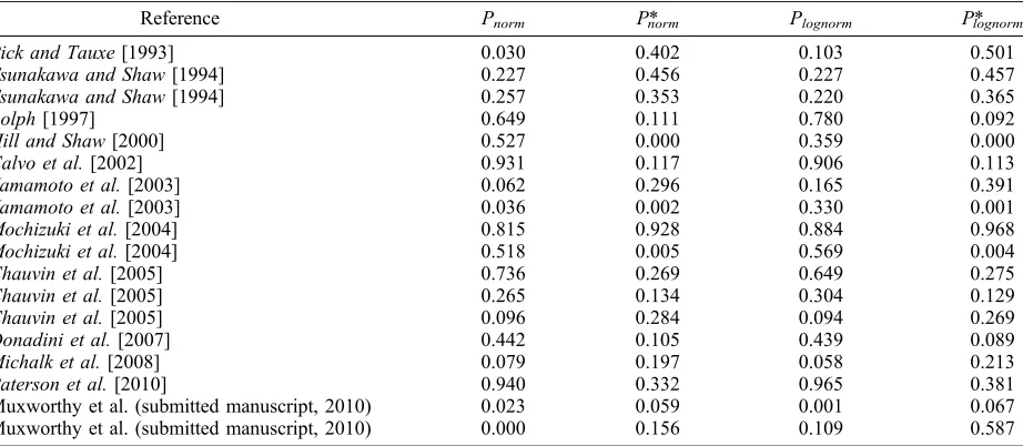
Table 2. Probability That the Investigated Data Sets Are Normally or Lognormally Distributeda

Reference Pnorm P*norm Plognorm P*lognorm

Pick and Tauxe[1993] 0.030 0.402 0.103 0.501

Tsunakawa and Shaw[1994] 0.227 0.456 0.227 0.457

Tsunakawa and Shaw[1994] 0.257 0.353 0.220 0.365

Rolph[1997] 0.649 0.111 0.780 0.092

Hill and Shaw[2000] 0.527 0.000 0.359 0.000

Calvo et al.[2002] 0.931 0.117 0.906 0.113

Yamamoto et al.[2003] 0.062 0.296 0.165 0.391

Yamamoto et al.[2003] 0.036 0.002 0.330 0.001

Mochizuki et al.[2004] 0.815 0.928 0.884 0.968

Mochizuki et al.[2004] 0.518 0.005 0.569 0.004

Chauvin et al.[2005] 0.736 0.269 0.649 0.275

Chauvin et al.[2005] 0.265 0.134 0.304 0.129

Chauvin et al.[2005] 0.096 0.284 0.094 0.269

Donadini et al.[2007] 0.442 0.105 0.439 0.089

Michalk et al.[2008] 0.079 0.197 0.058 0.213

Paterson et al.[2010] 0.940 0.332 0.965 0.381

Muxworthy et al. (submitted manuscript, 2010) 0.023 0.059 0.001 0.067

Muxworthy et al. (submitted manuscript, 2010) 0.000 0.156 0.109 0.587

a_P

normandPlognormare the probabilities that the data sets have been drawn from a continuous normal or lognormal distribution, respectively,

according to the Anderson‐Darling test.Pnorm* andPlognorm* are the probabilities, obtained using the Anderson‐Darling test, that the data sets have

nonideal behavior can be difficult to exclude from data sets, this is a possibility. On the other hand, the

Kolmogorov‐Smirnov (KS) test is more sensitive

to deviations close to the median value of the dis-tribution (i.e., large numbers of data that deviate from normality close to the mean will reduce the calculated probability). The one‐sample KS test for normality and lognormality returns probabilities

≥0.138, using the estimated mean and estimated

standard deviation. This provides additional evi-dence that the data sets could be sampled from either a normal or lognormal distribution at the 0.05 significance level.

[24] For scalar paleointensities, given that the

intensity must be >0 for all practical purposes, the distributions must be non‐Gaussian. In general, paleointensity data sets could be lognormally

dis-tributed (Table 2). However, most data sets cannot be distinguished from a normal distribution. Our simulations indicate that treating lognormal data normally (i.e., using the arithmetic mean and the standard deviation, equations (1) and (2), respec-tively) produces statistics that behave in an approxi-mately normal fashion. Importantly these statistics and probabilities represent best‐case scenarios and in reality the confidence levels of these statistics will be lower. In addition, large deviations or systematic biases due to nonideal paleointensity behavior cannot be identified with these methods, and all statistics of paleointensity data rely on the assumption that such biases can be successfully identified and excluded from final data sets.

4.2. Implications for the Paleointensity Database

[25] While the SEprovides a better estimate of the

confidence interval around an estimated mean, the estimated standard deviation, s, remains useful for

paleointensity studies. In one respect, s can be

viewed as a measure of the fidelity of a paleo-magnetic recorder, by accounting for natural (or laboratory induced) variability of paleointensity results from a group of specimens. It should therefore retain its role as a paleointensity data selection criterion. However, additional considera-tions are necessary if sis to be used in this way.

[26] The known distribution of sample variances

for normally distributed data allows quantification of a confidence interval around s:

ffiffiffiffiffiffiffiffiffiffiffiffiffiffiffiffiffiffiffiffiffi n1

2 1

2;n1

ð Þ v

u u

t ss

ffiffiffiffiffiffiffiffiffiffiffiffiffiffiffiffiffi n1

2

2;n1

ð Þ v u u

t s; ð8Þ

where2₁

2;n1

ð Þand2

2;n1

ð Þare the two‐tailedc2

critical values with (n − 1) degrees of freedom at the (1 − ₂)th and ₂th percentiles. As illustrated by Figure 7a, the confidence intervals are large for small nand decrease asnincreases. For n= 2, the 95% confidence interval is 0.4s≤s≤31.9s, but for n = 30 the interval is only 0.8s ≤ s ≤ 1.3s. This

quantifies the intuitive notion that s is poorly

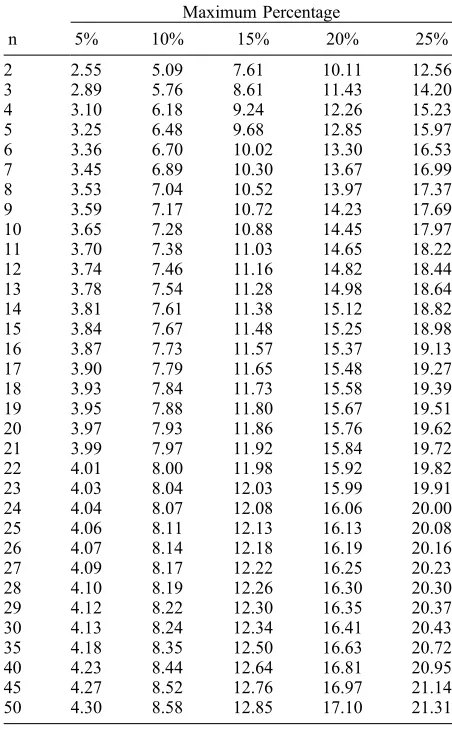
constrained for small n, for normally distributed data. If we wish to usesas a selection criterion for paleointensity analysis, we need to take into account the high degree of variability ofsfor small n. That is, criteria, such as dB (%), must have a sample size dependence, the necessity of which can be seen in Figure 6. If a staticdB (%) criterion were to be used, as is the case with most previous studies, a data set withn= 2 ands= 15% would be Table 3. Threshold Values for dBnThat Ensure a 95%

Confidence Level That the Estimated Standard Deviation Is Less Than a Specified Maximum Percentage of the Estimated Meana

n

Maximum Percentage

5% 10% 15% 20% 25%

2 2.55 5.09 7.61 10.11 12.56

3 2.89 5.76 8.61 11.43 14.20

4 3.10 6.18 9.24 12.26 15.23

5 3.25 6.48 9.68 12.85 15.97

6 3.36 6.70 10.02 13.30 16.53

7 3.45 6.89 10.30 13.67 16.99

8 3.53 7.04 10.52 13.97 17.37

9 3.59 7.17 10.72 14.23 17.69

10 3.65 7.28 10.88 14.45 17.97

11 3.70 7.38 11.03 14.65 18.22

12 3.74 7.46 11.16 14.82 18.44

13 3.78 7.54 11.28 14.98 18.64

14 3.81 7.61 11.38 15.12 18.82

15 3.84 7.67 11.48 15.25 18.98

16 3.87 7.73 11.57 15.37 19.13

17 3.90 7.79 11.65 15.48 19.27

18 3.93 7.84 11.73 15.58 19.39

19 3.95 7.88 11.80 15.67 19.51

20 3.97 7.93 11.86 15.76 19.62

21 3.99 7.97 11.92 15.84 19.72

22 4.01 8.00 11.98 15.92 19.82

23 4.03 8.04 12.03 15.99 19.91

24 4.04 8.07 12.08 16.06 20.00

25 4.06 8.11 12.13 16.13 20.08

26 4.07 8.14 12.18 16.19 20.16

27 4.09 8.17 12.22 16.25 20.23

28 4.10 8.19 12.26 16.30 20.30

29 4.12 8.22 12.30 16.35 20.37

30 4.13 8.24 12.34 16.41 20.43

35 4.18 8.35 12.50 16.63 20.72

40 4.23 8.44 12.64 16.81 20.95

45 4.27 8.52 12.76 16.97 21.14

50 4.30 8.58 12.85 17.10 21.31

a

accepted for further analysis along with a data set withn = 30 ands= 15%. In reality for the former data set, at the 95% confidence level,scould range from 6% to 479%, while for the latter data set, s will lie within the range 12%–20%. Clearly, then= 30 data set is more reliable. If we imposedB (%)≤ 25% both data sets would be deemed as acceptable results.

[27] The ratio m

ffiffi

n

p

s can be shown to follow a

non-centralt distribution with noncentrality parameter =pffiffin(Appendix C). This allows a sample size– dependent within‐site criterion (dBn (%)) to be

defined:

t

nc1;n1; ffiffin

p

Bnð Þ%

_¼ pffiffiffin

Rmax; ð9Þ

wheret

nc1;n1; _Bnp_{ð Þ}ffiffin_%is the one‐tailed noncentral

t critical value with noncentrality parameter _Bpffiffin nð%Þ,

and whereRmaxis the desired maximum acceptable

within‐site consistency (e.g., the commonly used threshold of ≤25%). This formulation exactly cor-responds to the confidence level contours for the normal distribution shown in Figure 6. Due to the fact thatdBn(%) is within the noncentrality

param-eter, no unique analytical solution can be derived, however, accurate solutions can be rapidly obtained using a numerical approach. The cutoff values that give 95% confidence that s

m≤25% for normally and

lognormally distributed data are shown in Figure 7b. Table 3 provides dBn(%) values for various

maxi-mum values of _ms andn, assuming normally distrib-uted data. Implementing a sample size–dependent within‐site consistency criterion ensures a consistent confidence level (e.g., 95%) in all selected data. Assuming normality, and choosing a maximum

within‐site consistency of 25%, this approach

gives a cutoff value forn= 2 ofdBn(%)≤12.56%,

and forn = 30,dBn(%)≤20.43% (Figure 7b and

Table 3).

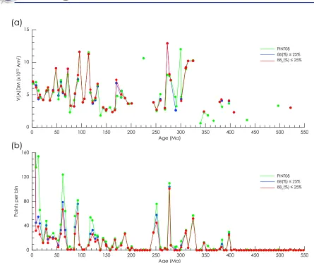
[28] The PINT08 paleointensity database [Biggin et

al., 2009] contains 3576 data entries. For the pur-poses of analyzing long‐term global paleointensity variations it is necessary to compare intensities in the form of virtual (axial) dipole moments (V(A) DM). Currently, only 3049 of the PINT08 entries report a V(A)DM. Using only these entries and excluding data entries withn = 1 and data with no reportednors, 2173 entries remain. If we applydB (%)≤25%, 1936 entries remain. This is, generally speaking, the extent to which most database anal-yses go, although some analanal-yses impose restric-tions on the paleointensity method used. If we apply the above‐described sample size–dependent within‐site criterion,dBn(%), 1560 data entries are

left; which represents ∼44% of all available data.

This a further reduction of ∼12% when compared

to using the dB (%) criterion. The result of this pruning of the database, however, is that we have a consistent confidence in the remaining data, despite

having variable n. The application of this new

criterion does not greatly change the general long‐ term trends in geomagnetic field intensity

varia-tion (Figure 8a). It does, however, exacerbate the problem of scarce data is certain time periods: no data are available in the Middle to Upper Triassic

(244–202 Ma) and only two data points pass the

dBn(%) criterion from the Lower Devonian to the

end of the Proterozoic Eon, from∼524–407 Ma. A more detailed view of the number of data accepted before and after applying the dBn (%) criterion is

shown in Figure 8b.

4.3. How Many Samples Are Enough?

[29] Determining the optimal number of samples

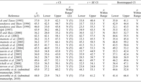
for a paleointensity study often is a subjective determination that depends on the degree of con-fidence required for the study in question. As outlined above, as many as 24 samples would be the optimal minimum number, but this is rarely achievable. When only one data point is available, no information can be obtained to quantify the uncertainty. Therefore, a minimum ofn= 2 should be used. This at least allows calculation of s and quantification of a confidence interval, despite this interval being large. However, investigators should aim to maximize the number of successful results by collecting as many paleomagnetic samples as Table 4. Confidence Intervals Around the Estimated Mean Using ±1sand ±t×SEand Estimated Using a Statistical Bootstrap Approacha

Reference

m (mT)

sCI t×SECI Bootstrapped CI

Lower Upper m Within Rangeb

(2s) Lower Upper m Within

Range Lower Upper m Within Range

Pick and Tauxe[1993] 37.0 31.9 42.3 Y (Y) 33.8 40.4 Y 35.0 41.1 Y

Tsunakawa and Shaw[1994] 45.5 42.5 44.7 N (Y) 33.7 53.5 Y 42.9 44.4 N

Tsunakawa and Shaw[1994] 46.0 33.0 45.8 N (Y) 23.5 55.3 Y 32.1 43.5 N

Rolph[1997] 43.9 30.2 48.2 Y (Y) 34.9 43.5 N 35.5 43.3 N

Hill and Shaw[2000] 36.2 28.0 35.2 N (Y) 30.5 32.7 N 30.5 32.7 N

Calvo et al.[2002] 42.3 42.1 58.1 Y (Y) 42.7 57.5 N 44.6 55.5 N

Yamamoto et al.[2003] 36.2 31.5 47.3 Y (Y) 33.3 45.5 Y 35.4 45.4 Y

Yamamoto et al.[2003] 36.2 37.7 66.1 N (Y) 45.3 58.5 N 46.8 59.2 N

Mochizuki et al.[2004] 45.5 41.7 51.1 Y (Y) 41.5 51.3 Y 43.5 50.4 Y

Mochizuki et al.[2004] 45.5 46.9 55.1 N (Y) 48.7 53.3 N 49.2 53.2 N

Chauvin et al.[2005] 36.0 34.8 43.8 Y (Y) 33.7 44.9 Y 35.3 42.4 Y

Chauvin et al.[2005] 36.0 35.6 43.0 Y (Y) 35.9 42.7 Y 37.1 42.4 N

Chauvin et al.[2005] 36.2 28.7 38.5 Y (Y) 28.5 38.7 Y 30.0 36.9 Y

Donadini et al.[2007] 49.6 43.7 52.1 Y (Y) 46.1 49.7 Y 46.2 49.6 Y

Michalk et al.[2008] 52.0 36.5 50.1 N (Y) 32.5 54.1 Y 36.4 47.1 N

Paterson et al.[2010] 24.0 23.1 25.5 Y (Y) 23.8 24.8 Y 23.9 24.8 Y

Muxworthy et al. (submitted manuscript, 2010)

45.0 37.2 60.2 Y (Y) 44.3 53.1 Y 44.6 52.8 Y

Muxworthy et al. (submitted manuscript, 2010)

44.0 23.9 74.3 Y (Y) 37.0 61.2 Y 41.4 66.4 Y

a_{CI, confidence interval.} b

possible per unit investigated. Studies that collect only a few paleomagnetic samples per unit (i.e., 10 or less) are most likely to produce data sets that have large or unquantifiable confidence intervals. Given that paleointensity studies can have high

failure rates, as many as 30–40 paleomagnetic

samples should be collected per unit.

4.4. Comparison of Confidence Intervals [30] When applied to real data sets, how well do the

confidence intervals defined by theSEcompare to other methods of estimating confidence intervals? The uncertainty interval defined by the estimated standard deviation, and the confidence intervals defined by the standard error (t×SE) and estimated by a nonparametric statistical bootstrap for the data sets in Table 1 are summarized in Table 4. Botht× SE and the bootstrapped confidence limits reflect the 95% confidence level, while the uncertainty interval of the standard deviation, under ideal cir-cumstances, reflects ∼68% coverage (i.e.,∼68% of the data will fall within ±1sof the estimated mean). Two standard deviations, which should represent

∼95% coverage is also included in Table 4,

how-ever, 2s is rarely used in paleointensity studies. The uncertainty intervals defined by the estimated standard deviation and the confidence interval defined by t × SE involve the assumption that the data sets are normally distributed. The bootstrapped confidence intervals involve no assumptions about the distribution of the data sets.

[31] Using the estimated standard deviation to

define uncertainty intervals includes the true mean for 12 of the 18 data sets investigated. This uncertainty interval fails when there is a bias in the data [e.g., Hill and Shaw, 2000] or when the data set contains few values [e.g.,Michalk et al., 2008]. The 2s uncertainty intervals include min all cases, but in some instances 2sdefines a range of ±50mT (e.g., the Vesuvius data of Muxworthy et al. (submitted manuscript, 2010)). In addition, it is unlikely that the estimated standard deviation will represent a consistent confidence level for data sets withn< 7 (Figure 4). Therefore, for at least six data sets the estimated standard deviation does not

provide 95% coverage (Table 4). The t × SE

con-fidence intervals include the true mean for 13 of the data sets and include the true mean whennis small.

Four of the five data sets for which the t × SE

confidence interval does not include mare rejected by the AD test for being normally or lognormally distributed about the expected means at the 0.05 significance level. This suggests that there may be a

bias in the data sets as noted by the authors [Hill and Shaw, 2000;Yamamoto et al., 2003;Mochizuki et al., 2004]. For these data sets, ±1s also fails to include the true mean.Rolph[1997] noted that the paleointensity results from the 1971 lava flow from Mt. Etna may be affected by chemical rem-anent magnetization. Despite having relatively large n(≥7), these five data sets yield inaccurate results (intensity error fraction, ∣IEF∣ ≥ 10.7% (Table 1)).

[32] The statistical bootstrap confidence intervals

were determined using a bias‐corrected accelerated

bootstrap method [Manly, 2007] with 106 repeat

samplings to define the 95% confidence interval around the mean (Table 4). The bootstrap method consistently fails to yield confidence intervals that include the true mean. It has been noted by others that the bootstrap method can underestimate the uncertainties of data sets with few values [e.g., Schenker, 1985]. A comparison between bootstrap andt×SEconfidence intervals from a Monte Carlo analysis of a normal distribution suggests that 20 point values are required for the bootstrap con-fidence interval to be within 10% of that defined by t×SE, and as many as 40 point values are needed to reduce this to within 5%. This makes bootstrapped confidence intervals unsuitable for most paleointensity data sets.

5. Conclusions

[33] We have assessed the calculation of

appropri-ate confidence intervals for paleointensity data using theoretical and numerical approaches, as well as using real data sets. More statistical consider-ation is required when analyzing paleointensity data than is generally used in such studies. Statistical analysis of real paleointensity data sets indicates that, in general, paleointensity data can be approxi-mated by normal or lognormal distributions around the expected values, irrespective of the method or material used. Exclusion of directional informa-tion, which precludes negative values, makes scalar paleointensity data fundamentally non‐Gaussian. Despite this, owing to small sample sizes and low standard deviations of the underlying distributions, the data can be approximated to be normally dis-tributed. This approximation fails when the data suffer from undetected bias and requires that paleointensity selection criteria successfully exclude nonideal behavior.

[34] Using a combination of analytical and

standard deviation alone is insufficient to provide a consistent confidence level when quantifying the uncertainty of a mean paleointensity estimate. Instead, the 95% confidence interval defined by the standard error (t ₁

2;n1

ð Þ×SE) should be used

as the uncertainty estimate for a mean paleointensity estimate. This ensures that the same confidence level is maintained when comparing data sets of different sizes, which is not the case for the esti-mated standard deviation whenn< 7. Comparisons indicate that use of the standard error to define the confidence interval around an estimated paleointensity provides a better uncertainty esti-mate than the estiesti-mated standard deviation or a statistical bootstrap. The estimated standard devi-ation should, however, still be used as a data selection criterion; it provides a measure of the variation from a paleomagnetic recorder. In order to maintain a consistent confidence level, criteria

such as dB (%) should incorporate a sample size

dependence. This is needed to reflect the larger uncertainties associated with standard deviation estimates based on smalln. Using a new criterion defined here (dBn(%)) considerably reduces the

paleointensity database available for long‐term geomagnetic analysis; however, it provides a con-sistent and more rigorous confidence level in the data that remain.

[35] In using both the estimated standard deviation

and the standard error for analyzing paleointensity data, authors should explicitly state in which form the uncertainties are presented. As a general rec-ommendation, we encourage authors to maintain the typically used approach and report paleointensity estimates ± one estimated standard deviation, along with n. This allows the standard error to be calcu-lated and helps to maintain consistent data reporting. In addition, we recommend that the standard error is referred to as such, and not as the standard deviation of the mean, which can cause confusion with the estimated standard deviation,s.

[36] With respect to the question of how many

sam-ples are enough to obtain a reliable paleointensity estimate, the expression“safety in numbers”remains true. Ideally, at least 24 acceptable paleointensity results are desirable, although this has rarely been achieved in the published literature. The lack of

any quantifiable uncertainty when n = 1 should

automatically preclude these data sets from any

meta‐analysis; therefore n = 2 is the minimum

sample size. Given the typically high failure rates, paleointensity studies should endeavor to collect a

minimum of 30–40 paleomagnetic samples per

flow (or stratigraphic level) in the hope of obtain-ing at least of 7–8 acceptable results. Collection of fewer paleomagnetic samples can lead to acquisi-tion of data sets that have large confidence inter-vals or that are insufficient to provide reliable estimated means and uncertainties (i.e., whenn= 1). Modern methods that enable analysis of larger numbers of paleomagnetic samples, such as the microwave technique, should aid investigators in achieving this goal.

Appendix A: Accuracy of the Estimated

Mean

[37] We wish to identify the probability of

obtain-ing an estimated mean,m, that falls within ±10% of the true mean m:

Pð0:9m1:1Þ: ðA1Þ

This can be calculated using the normal cumulative distribution function (CDF; fnorm):

P¼fnorm 1:1; ; _ffiffiffi

n

p

fnorm 0:9; ; _ffiffiffi

n

p

; ðA2Þ

where ffiffi

n

p is the standard deviation of the sample

means.

Appendix B: Confidence Intervals

[38] To determine the usefulness of the estimated

standard deviation to define confidence intervals, we calculate the probability that m lies within an interval around m that is defined by a multiple (i) of s, i.e.,

PðismþisÞ: ðB1Þ

Rearranging and multiplying throughout by pffiffiffin, we obtain:

PðismþisÞ ¼P ipffiffiffinm_sffiffi

n p i

ffiffiffi n

p !

:

ðB2Þ

Here m follows a normal distribution and psffiffi_n a c

distribution, the ratio of which is t distributed, with n − 1 degrees of freedom. The t distribution CDF (ft) can be used to calculate the probabilities:

P¼ft i

ffiffiffi n

p

; n1

ft i

ffiffiffi n

p

; n1

For the confidence intervals using the standard error (SE), a similar approach can be used:

PðiSEmþiSEÞ

¼P isffiffiffi n

p m isffiffiffi n

p

¼P im_sffiffi

n p i

!

: ðB4Þ

Hence:

P¼ftði;n1Þ ftði;n1Þ: ðB5Þ

[39] The numerical simulations for lognormally

distributed data have a probability variation that

depends on the true standard deviation, s. For

both the estimated standard deviation and standard error probabilities (Figures 4 and 5), this depen-dence produces a maximum probability difference

of∼10% assvaries from 1% to 100%. Maximum

probability difference contour plots are given in Figure B1.

Appendix C: Within

‐

Site Consistency

[40] We wish to consider the probability that the

ratio of the estimated standard deviation to the estimated mean (_ms) is less than a specified value (Rmax), say≤0.25:

P s mRmax

: ðC1Þ

If we consider a noncentral t distribution:

TncZ

þ_ffiffiffi V

q ; ðC2Þ

where Zis a standard normal distribution, is the noncentrality parameter, and V is ac2 distribution

with n degrees of freedom. Given the known

dis-tributions ofmands2(see section 2), we can show that:

Zm_ffiffi

n

p ; ðC3Þ

and

ffiffiffiffi V

r

ffiffiffiffiffiffiffiffiffiffiffiffiffiffiffiffiffiffiffi s2ðn1Þ

2_ðn1Þ

s

¼s: ðC4Þ

Therefore, pffiffinðmÞþ

s is distributed according to a

noncentralt distribution. It can then be shown that

mpffiffin

s is also noncentral t distributed provided that:

¼

ffiffiffi n

p

: ðC5Þ

Hence:

P s mRmax

¼P m ffiffiffi n

p

s ffiffiffi n

p

Rmax

; ðC6Þ

which can be calculated using the noncentral t

distribution CDF (fnct):

P¼fnct

ffiffiffi n

p

Rmax;n1;

: ðC7Þ

Acknowledgments

[41] This study was funded by the Royal Society and JSPS. We thank Alan Kimber, Richard Lockhart, and Robin Willinck for statistical advice and Lisa Tauxe for providing data. We are grateful to Andrew Roberts for his comments and advice. We thank Josh Feinberg, Yongjae Yu, and two anonymous reviewers for their helpful comments that improved this paper.

References

Aitchison, J., and J. A. C. Brown (1957), The Lognormal Distribution, Cambridge Univ. Press, Cambridge, U. K. Anderson, T. W., and D. A. Darling (1952), Asymptotic theory

of certain“goodness of fit”criteria based on stochastic pro-cesses,Ann. Math. Stat.,23, 193–212.

Biggin, A. J., H. N. Böhnel, and F. R. Zúñiga (2003), How many paleointensity determinations are required from a single lava flow to constitute a reliable average?,Geophys. Res. Lett.,30(11), 1575, doi:10.1029/2003GL017146.

Biggin, A. J., G. H. M. A. Strik, and C. G. Langereis (2009), The intensity of the geomagnetic field in the late‐Archaean: New measurements and an analysis of the updated IAGA palaeointensity database,Earth Planets Space, 61, 9–22. Calvo, M., M. Prévot, M. Perrin, and J. Riisager (2002),

Inves-tigating the reasons for the failure of palaeointensity experi-ments: A study on historical lava flows from Mt. Etna (Italy), Geophys. J. Int., 149, 44–63, doi:10.1046/j.1365-246X. 2002.01619.x.

Chauvin, A., P. Roperch, and S. Levi (2005), Reliability of geomagnetic paleointensity data: The effects of the NRM fraction and concave‐up behavior on paleointensity determi-nations by the Thellier method,Phys. Earth Planet. Inter., 150, 265–286, doi:10.1016/j.pepi.2004.11.008.

Coe, R. S. (1967), Paleo‐intensities of the Earth’s magnetic field determined from Tertiary and Quaternary rocks,J. Geo-phys. Res.,72, 3247–3262, doi:10.1029/JZ072i012p03247. Donadini, F., M. Kovacheva, M. Kostadinova, L. Casas, and

L. J. Pesonen (2007), New archaeointensity results from Scandinavia and Bulgaria: Rock‐magnetic studies inference and geophysical application,Phys. Earth Planet. Inter., 165, 229–247, doi:10.1016/j.pepi.2007.10.002.

Fabian, K. (2009), Thermochemical remanence acquisition in single‐domain particle ensembles: A case for possible over-estimation of the geomagnetic paleointensity,Geochem. Geophys. Geosyst.,10, Q06Z03, doi:10.1029/2009GC002420. Hill, M. J., and J. Shaw (2000), Magnetic field intensity study of the 1960 Kilauea lava flow, Hawaii, using the microwave palaeointensity technique,Geophys. J. Int.,142, 487–504, doi:10.1046/j.1365-246x.2000.00164.x.

Manly, B. F. J. (2007),Randomization, Bootstrap and Monte Carlo Methods in Biology, 3rd ed., 455 pp., Chapman and Hall, Boca Raton, Fla.

Maus, S., et al. (2005), The 10th‐Generation International Geomagnetic Reference Field,Geophys. J. Int.,161, 561– 565, doi:10.1111/j.1365-246X.2005.02641.x.

Michalk, D. M., A. R. Muxworthy, H. N. Böhnel, J. Maclennan, and N. R. Nowaczyk (2008), Evaluation of the multispecimen parallel differential pTRM method: A test on historical lavas from Iceland and Mexico,Geophys. J. Int.,173, 409–420, doi:10.1111/j.1365-246X.2008.03740.x.

Mochizuki, N., H. Tsunakawa, Y. Oishi, S. Wakai, K. Wakabayashi, and Y. Yamamoto (2004), Palaeointensity study of the Oshima 1986 lava in Japan: Implications for the reliability of the Thellier and LTD‐DHT Shaw methods,Phys. Earth Planet. Inter., 146, 395–416, doi:10.1016/j. pepi.2004.02.007.

Paterson, G. A., A. R. Muxworthy, A. P. Roberts, and C. Mac Niocaill (2010), Assessment of the usefulness of lithic clasts from pyroclastic deposits for paleointensity determination, J. Geophys. Res.,115, B03104, doi:10.1029/2009JB006475. Perrin, M. (1998), Paleointensity determination, magnetic domain structure, and selection criteria,J. Geophys. Res., 103, 30,591–30,600, doi:10.1029/98JB01466.

Pick, T., and L. Tauxe (1993), Geomagnetic palaeointensities during the Cretaceous normal superchron measured using s u b m a r i n e b a s a l t i c g l a s s , N a t u r e, 3 6 6, 2 3 8–2 4 2 , doi:10.1038/366238a0.

Riisager, P., R. Waagstein, J. Riisager, and N. Abrahamsen (2002), Thellier palaeointensity experiments on Faroes flood basalts: Technical aspects and geomagnetic implications, Phys. Earth Planet. Inter., 131, 91–100, doi:10.1016/ S0031-9201(02)00031-6.

Rolph, T. C. (1997), An investigation of the magnetic variation within two recent lava flows,Geophys. J. Int.,130, 125–136, doi:0.1111/j.1365-246X.1997.tb00992.x.

Schenker, N. (1985), Qualms about bootstrap confidence inter-vals,J. Am. Stat. Assoc.,80, 360–361.

Shaw, J. (1974), A new method of determining the magnitude of the palaeomagnetic field: Application to five historic lavas and five archaeological samples,Geophys. J. R. Astron. Soc., 39, 133–141, doi:10.1111/j.1365-246X.1974.tb05443.x. Stephens, M. A. (1974), EDF statistics for goodness of fit and

some comparisons,J. Am. Stat. Assoc.,69, 730–737. Stephens, M. A. (1979), Tests of fit for the logistic distribution

based on the empirical distribution function,Biometrika,66, 591–595, doi:10.1093/biomet/66.3.591.

Stephens, M. A. (1986), Tests based on EDF statistics, in Goodness‐of‐Fit Techniques, edited by R. B. D’Agostino and M. A. Stephens, pp. 97–194, Marcel Dekker, New York. Tanaka, H., and M. Kono (1991), Preliminary results and reli-ability of palaeointensity studies on historical and14C dated Hawaiian lavas,J. Geomagn. Geoelectr.,43, 375–388. Thellier, E., and O. Thellier (1959), Sur l’intensité du champ

magnétique terrestre dans le passé historique et géologique, Ann. Geophys.,15, 285–376.

Tsunakawa, H., and J. Shaw (1994), The Shaw method of palaeointensity determinations and its application to recent volcanic rocks,Geophys. J. Int.,118, 781–787, doi:10.1111/ j.1365-246X.1994.tb03999.x.

Walton, D., J. Share, T. C. Rolph, and J. Shaw (1993), Micro-wave magnetisation, Geophys. Res. Lett., 20, 109–111, doi:10.1029/92GL02782.

Yamamoto, Y. (2006), Possible TCRM acquisition of the Kilauea 1960 lava, Hawaii: Failure of the Thellier paleoin-tensity determination inferred from equilibrium temperature of the Fe‐Ti oxide,Earth Planets Space,58, 1033–1044. Yamamoto, Y., H. Tsunakawa, and H. Shibuya (2003),