COMPUTING BRAID GROUPS OF GRAPHS WITH APPLICATIONS TO ROBOT MOTION PLANNING

Homology, Homotopy and Applications, vol. 14(1), 2012, pp.159–180

COMPUTING BRAID GROUPS OF GRAPHS WITH

APPLICATIONS TO ROBOT MOTION PLANNING

VITALIY KURLIN

(communicated by Robert Ghrist)

Abstract

An algorithm is designed to write down presentations of graph braid groups. Generators are represented in terms of actual motions of robots moving without collisions on a given connected graph. A key ingredient is a new motion planning algorithm whose complexity is linear in the number of edges and is quadratic in the number of robots. The computing algo-rithm implies that 2-point braid groups of all light planar graphs have presentations where all relators are commutators.

1.

Introduction

1.1. Brief summary

This is a research on the interface between topology and graph theory with applica-tions to motion planning algorithms in robotics. Consider moving objects as zero-size points that travel without collisions along fixed tracks that form a connected graph, say on a factory floor or road map. These objects will be called ‘robots’, although the reader may use a more neutral and abstract word like ‘token’.

For practical reasons, discrete analogues of configuration spaces of graphs are stud-ied. Then robots can not be very close to each other, at least one full open edge apart. This discrete approach reduces the motion planning of real (not zero-size) vehicles to combinatorial questions about ideal robots that move on a subdivided graph.

1.2. Graphs and theirs configuration spaces

Let us recall basic notions. Agraph Gis a 1-dimensional finite CW complex whose 1-cells are supposed to be open. The 0-cells and open 1-cells are calledvertices and edges, respectively. If the endpoints of an edge e are the same, then e is called a loop. Amultiple edge is a collection of edges with the same distinct endpoints. The topologicalclosure ¯eof an edgeeis the edgeeitself with its endpoints.

Thedegree degv of a vertex v is the number of edges attached tov, i.e., a loop contributes 2 to the degree of its vertex. Vertices of degree 1 or 2 arehanging ortrivial, respectively. Vertices of degree at least 3 areessential. A path (acycle, respectively)

Received November 4, 2009, revised June 8, 2011; published on June 4, 2012. 2000 Mathematics Subject Classification: 57M05, 20F36, 05C25.

Key words and phrases: graph, braid group, configuration space, fundamental group, homotopy type, deformation retraction, collision free motion, planning algorithm, complexity, robotics.

Article available athttp://intlpress.com/HHA/v14/n1/a8anddoi:10.4310/HHA.2012.v14.n1.a8

Copyright c⃝2012, International Press. Permission to copy for private use granted.

This is the modified version of the paper published in

of a lengthk in Gis a subgraph that consists ofk edges and is homeomorphic to a segment (a circle, respectively). Atree is a connected graph without cycles.

The direct product Gn_{=G×· · ·×G (n times) has the product structure of a} ‘cubical’ complex such that each product ¯c1×· · ·×c¯n is isometric to a Euclidean cube [0,1]k_{, where ¯c}

i is the topological closure of a cell ofG. The dimension kis the number of the cellsci that are edges ofG. Thediagonal of the productGn is

∆(Gn) ={(x1, . . . , xn)∈Gn|xi=xj for somei̸=j}.

Definition 1.1. Let Gbe a graph, n be a positive integer. Theordered topological configuration spaceOC(G, n) ofndistinct robots inGisGn_−∆(Gn_{). Theunordered} topological configuration space UC(G, n) of n indistinguishable robots in G is the quotient ofOC(G, n) by the action of the permutation groupSn ofnrobots.

The ordered topological spaceOC([0,1],2) ={(x, y)∈[0,1]2|x̸=y} is the unit square without its diagonal. This space is homotopy equivalent to a disjoint union of two points. SpacesX, Y arehomotopy equivalent if there are continuous maps

f:X →Y, g:Y →X such that g◦f:X→X, f◦g:Y →Y

can be connected with the identity maps idX: X→X, idY: Y →Y, respectively, through continuous families of maps. In particular,X iscontractibleifX is homotopy equivalent to a point. A spaceX can be homotopy equivalent to its subspace Y by a deformation retraction that is a continuous family of maps ft:X →X, t∈[0,1], such thatft|Y = idY, i.e., all ftare fixed onY,f0= idX andf1(X) =Y.

The unordered topological space UC([0,1],2)_≈{(x, y)_∈[0,1]2

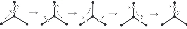
|x < y_} is con-tractible to a single point. More generally, OC([0,1], n) has n! contractible con-nected components, while UC([0,1], n) deformation retracts to the standard con-figuration xi = (i−1)/(n−1), i= 1, . . . , n, in [0,1]. If a connected graph G has a vertex of degree at least 3, then the configuration spacesOC(G, n), UC(G, n) are path-connected. Swap robotsx, ynear such a vertex as shown in Figure 1.

x

x x

x x

y y

y y

y

Figure 1: Swapping two robotsx, y without collisions on the tripodT

Definition 1.2. Given a connected graphGhaving a vertex of degree at least 3, the graph braid groups P(G, n) and B(G, n) are the fundamental groups π1(OC(G, n))

andπ1(UC(G, n)), respectively, where arbitrary base points are fixed.

For the tripodT in Figure 1, both configuration spacesOC(T,2), UC(T,2) are homotopy equivalent to a circle; see Example 2.1, i.e., B(T,2)∼=Z, P(T,2)∼=Z, althoughP(T,2) can be considered as an index 2 subgroup 2ZofB(T,2)∼=Z. Definition 1.3. The ordered discrete space OD(G, n) consists of all the products ¯

The support supp(H) of a subset H_⊂G is the minimum union of closed cells containingH. For instance, the support of a vertex or an open edge coincides with its topological closure in the graph G. The support of a point interior to an open edgee is ¯e, i.e., the edge ewith its endpoints. A configuration (x1, . . . , xn)∈Gn is

safeif supp(xi)∩sup(xj) =∅wheneveri̸=j. Then the discrete configuration space OD(G, n) consists of all safe configurations:

OD(G, n) ={(x1, . . . , xn)∈Gn |supp(xi)∩supp(xj) =∅, i̸=j}.

A path in a graphGisessentialif the path connects distinct vertices of degrees not equal to 2. A cycle inGisessential if the cycle contains a vertex of a degree more than 2. Since only connected graphs are considered, a non-essential cycle coincides with the whole graph. Subdivision Theorem 1.4 provides sufficient conditions such that the configuration spaces OC(G, n),UC(G, n) deformation retract to their discrete analoguesOD(G, n),UD(G, n), respectively. ThenB(G, n)∼=π1(UD(G, n)).

Theorem 1.4 ([1, Theorem 2.1]).Let Gbe a connected graph, n!2. The discrete spacesOD(G, n),UD(G, n)are deformation retracts of the topological configuration spacesOC(G, n),UC(g, n), respectively, if both conditions (1.4a) and (1.4b) hold:

(1.4a) Every essential path inGhas at least n+ 1 edges; (1.4b) Every essential cycle inGhas at leastn+ 1 edges.

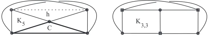
The conditions above imply thatG has at least n vertices, so OD(G, n)_̸=_∅. A strengthened version of Subdivision Theorem 1.4 forn= 2 only requires that Ghas no loops and multiple edges [1, Theorem 2.4]. The topological configuration spaces of two points on the Kuratowski graphs K5, K3,3 in Figure 2 deformation retract

to their smaller discrete analogues. InOD(K5,2), if the first robot is moving along

an edge h∈K5, then the second robot can be only in the triangular cycle C⊂

K5−h. In total, these ten triangular tubesh×Cform the oriented surface of genus

6. Similarly, computing the Euler characteristic, we conclude thatOD(K3,3,2) is the

oriented surface of genus 4. These are the only graphs without loops whose discrete configuration spacesOD(G,2) are closed manifolds; see [1, Corollary 5.8].

Students of L. Sabalka [12] have extended Subdivision Theorem 1.4 for anyn >2 to the optimal criterion wheren+ 1 is replaced byn−1 in condition (1.4a).

Figure 2: Kuratowski graphsK5 andK3,3

1.3. Main results

a nice global structure of the group and proves that all graph braid groups are torsion free [1, Corollary 3.7 on p. 25]. The latter approach is based on the discrete Morse theory developed by Forman [7]. One writes presentations of graph braid groups by retracting a big discrete configuration space to a smaller subcomplex.

This paper proposes another local approach based on the classical Seifert–van Kampen Theorem 3.1. Presentations are computed step-by-step starting from simple graphs and adding edges one-by-one, which allows us to update growing networks in real-time. Resulting Algorithm 1.5 expresses generators of graph braid groups using actual motions of robots, i.e., as a list of positions at discrete time moments. The key ingredient is new motion planning Algorithm 4.3 to connect any configurations ofnrobots. The computational complexity of Algorithm 4.3 is linear in the number of edges and is quadratic in the number of robots.

Algorithm 1.5. For a connected graph G, there is an algorithm to write down a presentation of the graph braid groupB(G, n). Generators are represented by actual paths between configurations; see step-by-step instructions in Subsection 4.1.

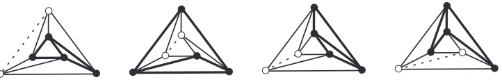
According to [6, Theorem 5.6], the braid groups of planar graphs having only disjoint cycles have presentations where each relator is a commutator, not necessarily a commutator of generators. To demonstrate the power of Algorithm 1.5, this result is extended to a wider class of light planar graphs. A planar connected graphGis called light if any cycleC⊂Ghas an open edge hsuch that all cycles fromG−¯hdo not meetC. Removing the closure ¯hfromGis equivalent to removing the endpoints ofh

and all open edges attached to the endpoints. Any loop or a multiple edge provides an edge h satisfying the above condition. Figure 3 shows a non-light planar graph with four choices of a (dashed) edge h and corresponding (fat) cycles from G₋¯h. Indeed, in each case the fat cycles fromG₋¯hmeet any cycleC containingh.

Figure 3: A non-light planar graph with four choices of a closed edge ¯h

Corollary 1.6.The braid groupB(G,2)of any light planar graphGhas a presenta-tion where each relator is a commutator of mopresenta-tions along disjoint cycles.

A stronger version of Corollary 1.6 with a geometric description of generators and relators is given in Proposition 4.8 in the case of unordered robots.

Outline

Acknowledgements

The author thanks the anonymous referee for helpful suggestions and Lucas Sabalka for his valuable corrections in Subsections 2.2, 3.1 and 4.2.

2.

Discrete configuration spaces of a graph

In this section discrete configuration spaces are discussed in more detail. These spaces are recursively constructed in Lemmas 2.5 and 2.6. Further assume that the number of robots isn!2.

2.1. Configuration spaces of the tripod T

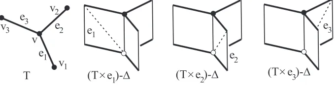
This subsection describes configuration spaces of two points on the tripodT. The tripod T consists of three hanging edges e1, e2, e3 that are attached to the central

vertexv; see Figure 4.

T

(T e )-

!

(T e )-

_!

(T e )-

!

e

e

e

e

e

e

v

v

v

v

1

1

1 1

2

3 2

2

2 3

3

3

Figure 4: The tripodT and (T_×e1)−∆, (T×e2)−∆, (T×e3)−∆

Example 2.1. The ordered topological space OC(T,2) is the union of three 3-page booksT×e1,T×e2,T×e3shown in the right-hand side pictures of Figure 4

with-out the diagonal ∆={(x, y)∈T2_{|x̸=y}. ThenOC(T,2) consists of the six}

sym-metric rectanglesei×ej (i̸=j) and six triangles from the squaresei×ei,i= 1,2,3, after removing their diagonals; see the left-hand side picture of Figure 5 and [2, Example 6.26].

Example 2.2. The ordered topological space OC(T,2) deformation retracts to the polygonal circle in the right-hand side picture of Figure 5. This circle is the ordered discrete space OD(T,2) having 12 vertices vi×vj (i̸=j) and v×vi, vi×v, i= 1,2,3, symmetric under the permutation of factors. The unordered spacesUC(T,2), UD(T,2) are the quotients of the corresponding ordered spaces by the rotation through π and are homeomorphic to OC(T,2),OD(T,2), respectively. Hence the graph braid groupsB(T,2)∼=Z,P(T,2)∼=Z can be computed by using the simpler discrete spacesUD(T,2),OD(T,2), which is reflected in Theorem 1.4.

2.2. Recursive construction of discrete spaces

OC

_(T,2)

OD

_(T,2)

e e

e e

e e

e e

e e

e e

e v

e v

e v

v e

v e

v e

v e

v e

v e

e v

e v

e v

e v

Figure 5: The ordered spaceOC(T,2) and its discrete analogueOD(T,2)

Example 2.3. Let us show how to construct the ordered space OD(T,2) adding the closed edge ¯e1to the subgraphT −(e1∪v1) = ¯e2∪¯e3≈[0,1]. If both robotsx, yare

not in the open edge e1, then (x, y)∈OD(T−e1,2), where T−e1≈v1∪e¯2∪¯e3,

i.e., eitherx=v1, y∈e¯2∪e¯3 (or vice versa) or (x, y)∈OD(¯e2∪¯e3,2). Sincexcan

not be close toyby Definition 1.3 (e.g., if x∈e1, theny∈{v2, v3}), then one has

OD(T,2)_≈OD(T₋e1,2)∪({v2, v3}×e¯1)∪(¯e1×{v2, v3}),

where

OD(T₋e1,2)≈OD(¯e2∪e¯3,2)∪!v1×(¯e2∪¯e3)"∪!(¯e2∪¯e3)×v1".

The subspace OD(T−e1,2) consists of four fat segments in the right-hand side

picture of Figure 5, where the two horizontal segments represent OD(¯e2∪¯e3,2).

Taking the quotient by swapping the robots, similarly decompose the unordered space

UD(T,2)_≈UD(¯e2∪¯e3,2)∪!(¯e2∪¯e3) ˜×v1"∪({v2, v3}ט e¯1).

HereA_ט Bdenotes the quotient of (A_×B)_∪(B_×A) over the symmetry that swaps the factors. The left-hand side picture of Figure 6 shows the subspace UD(¯e2∪

¯

e3,2)≈[0,1] and the whole spaceUD(T,2)≈S1. The segmentsv2טe¯1 andv3ט ¯e1

are glued at the endpointsv2ט v1, v3ט v1 andv2ט v, v3טv, respectively.

(e e) v e e

v e

v e

UD_{( ,2)} UD(G-e,n)

UD_{(G,n) :}

UD_{(G-Nbhd(e),n-1) e} UD_{(T,2) :}

1 1 1

2

2 3 3

2 3 ~ ~ ~ ~

Figure 6: Attaching the cylinder in the recursive construction ofUD(G, n)

instance, the complement to the neighbourhood Nbhd(e1) in the tripodT consists of

the hanging verticesv2, v3; see the left-hand side picture of Figure 4.

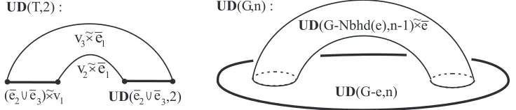
Example 2.4. Extending the recursive idea of Example 2.3, let us construct the or-dered 2-point spaceOD(G,2) of any connected graph G. Fix an open edge e_⊂G

with verticesu, v and consider the case when one of the robots, say y, stays in e. Thenx_∈G₋Nbhd(e) becausexcan not be in the same edgeeand also in the edges adjacent toe. If both robots x, y are not in e, then (x, y) is in the smaller ordered spaceOD(G−e,2). ThenOD(G,2) is a union of smaller subspaces:

OD(G,2)≈OD(G−e,2)∪!(G−Nbhd(e))×e¯"∪!¯e×(G−Nbhd(e))".

Here the first cylinder (G₋Nbhd(e))_ׯe is glued to OD(G₋e,2) along the sub-graphs (G−Nbhd(e))×uand (G−Nbhd(e))×v. The second cylinder is symmetric to the first one. Taking the quotient over swapping the factors, one gets

UD(G,2)≈UD(G−e,2)∪((G−Nbhd(e)) ˜×¯e),

whereA_ט B= ((A×B)∪(B×A))/∼. Lemmas 2.5 and 2.6 are discrete analogues of Ghrist’s construction of the ordered topological spaceOC(G, n) [8, Lemma 2.1].

Lemma 2.5. Let a connected graphG have an open edge ewith vertices u, v. Then the ordered discrete spaceOD(G, n)is homeomorphic to the union

OD(G, n)_≈OD(G₋e, n)_∪ni=1(OD(i)(G−Nbhd(e), n−1)ׯe),

where

OD(i)(G−Nbhd(e), n−1)×e¯={x∈OD(G, n)|xi∈e¯} is glued toOD(G−e, n)along

OD(i)(G−Nbhd(e), n−1)×u={x∈OD(G−Nbhd(e), n)|xi=u} and

OD(i)(G−Nbhd(e), n−1)×v={x∈OD(G−Nbhd(e), n)|xi=v}, i= 1, . . . , n.

Proof. In the spaceOD(G, n) of all safe configurationsx= (x1, . . . , xn) consider the

smaller subspace OD(G₋e, n), where xi∈/e for all i= 1, . . . , n. The complement OD(G, n)₋OD(G₋e, n) consists of configurations with xi ∈efor somei. By Def-inition 1.3 the other robotsxj∈/Nbhd(e) forj̸=i, i.e., the complement is

OD(G, n)₋OD(G₋e, n)_{≈ ∪}ni=1OD(i)(G−Nbhd(e), n−1)×e.

The bases of each cylinder above are subspaces of the smaller configuration space:

OD(i)(G−Nbhd(e), n−1)×u, OD(i)(G−Nbhd(e), n−1)×u⊂OD(i)(G−e, n).

The cylinderOD(i)(G−Nbhd(e), n−1)×erepresents motions when thei-th robot

products consisting of the factors A1, . . . , Ak over all orders and then quotient the union by the permutation groupSn. The result can be denoted byA1ט· · ·×˜ Ak. Lemma 2.6. Let a connected graphG have an open edge ewith vertices u, v. Then the unordered discrete spaceUD(G, n)is homeomorphic to (see Figure 6)

UD(G, n)_≈UD(G₋e, n)_∪(UD(G₋Nbhd(e), n₋1) ˜_ׯe),

where the subspaceUD(G−Nbhd(e), n−1) ˜×e¯is glued to UD(G−e, n)along UD(G₋Nbhd(e), n₋1) ˜_×u and UD(G₋Nbhd(e), n₋1) ˜_×v.

Proof. Quotient the ordered space from Lemma 2.5 by the permutation groupSn: OD(G, n) _{−−−−→}≈ OD(G₋e, n)_∪n

i=1(OD(i)(G−Nbhd(e), n−1)ׯe) quotient

⏐ ⏐

$ f

⏐ ⏐ $

UD(G, n) _{−−−−→}g UD(G₋e, n)_∪(UD(G₋Nbhd(e), n₋1) ˜_ׯe).

The natural projectionf above is continuous by the pasting lemma. The induced mapgis bijective and continuous by the universality property of quotients and defines a homeomorphism sinceUD(G, n) is compact, while its image is Hausdorff.

2.3. Homotopy types of configuration spaces

This subsection recalls general results on homotopy types of configuration spaces. A topological spaceX is called aspherical or a K(π,1) space, if the spaceX has a contractible universal cover, in particularπi(X) = 0 fori >1. A coveringp: Y _→X

isuniversal, if the coverY is simply connected. Then the coveringphas theuniversal property that, for any covering q:Z _→X, there is another covering Y _→Z whose composition withq:Z _→X gives the original coveringp:Y _→X.

Proposition 2.7(Asphericity of configuration spaces, Ghrist [8, Corollary 2.4, The-orem 3.1] for topological spaces and Abrams [1, Section 3.2] for discrete spaces). Every component ofOC(G, n),UC(G, n),OD(G, n),UD(G, n)is aspherical.

Ghrist [8, Corollary 2.4, Theorem 3.1] proves the above result for the ordered topo-logical spaceOC(G, n), which implies the same conclusion forUC(G, n), because the universal cover of a component ofUC(G, n) is a universal cover of some component ofOC(G, n) as mentioned by Abrams [1, the proof of Corollary 3.6].

Proposition 2.8 implies that the homotopy type of discrete spaces depends on the graphG, but not on the numbernof robots. It was proved by Ghrist [8, Theorems 2.6 and 3.3] forOC(G, n). The result easily extends to the unordered case.

The circleS1_{is excluded below, because its unordered spaceUC(S}1_{, n) is}

homo-topically equivalent to a circle, while OC(S1_{, n) deformation retracts to a disjoint}

union of (n₋1)! circles indexed by permutations ofnrobots up to cyclic shifts. Proposition 2.8 (Homotopy type of topological configuration spaces). If a con-nected graph G_̸≈S1 _{has exactly m essential vertices (of degree at least 3), then}

OC(G, n)andUC(G, n)deformation retract to m-dimensional complexes.

3.

Fundamental groups of unordered discrete spaces

In this section one computes graph braid groups. Namely, one shows how their presentations change by Seifert–van Kampen Theorem 3.1 after adding new edges to a graph. LetX, Y be open path-connected subsets ofX_∪Y such thatX_∩Y _̸=_∅is also path-connected. IfX, Y are not open inX_∪Y, then they usually can be replaced by their open neighbourhoods that deformation retract toX, Y, respectively. Assume thatX, Y, X_∩Y, X_∪Y have a common base point. Ifαis a finite vector of elements, then a group presentation has the form_⟨α_|ρ_⟩, where the relatorρ(a vector of words in the alphabetα) denotes the vector relationρ= 1. A practical reformulation of the Seifert–van Kampen Theorem is below.

Theorem 3.1 (Seifert–van Kampen Theorem [3, Theorem 3.6 on p. 71]). If presen-tations π1(X)∼=⟨β|λ⟩, π1(Y)∼=⟨γ|µ⟩ are given and π1(X∩Y) is generated by

(a vector of ) words α, then the groupπ1(X∪Y)has the presentation π1(X∪Y)∼=

⟨β,γ_|λ,µ,αX=αY⟩, where αX,αY are obtained from the words α by rewriting the wordsαin the alphabetsβ,γ, respectively.

As an example, consider the 2-dimensional torus X∪Y, where X is the com-plement to a closed disk D, while Y is a open neighbourhood of D, i.e., X∩Y

is an annulus. Then X is homotopically equivalent to a wedge of two circles, i.e., π1(X)∼={α,β| }is free,π1(Y)∼=⟨|⟩is trivial andπ1(X∩Y)∼=Z, hence

π1(X∪Y)∼={α,β|αβα−1β−1}

asαβα−1_β−1 _{represents the boundary ofD.}

Presentations of the groupsπ1(UD(G, n))∼=B(G, n) will be written down

step-by-step by adding edges to the graph and by monitoring changes in the presentations. The base of our recursive computation is the contractible space UD([0,1], n) of n

robots in a segment whose fundamental group is trivial.

In Proposition 3.2 one glues a hanging edge to a vertex of degree at least 2, e.g., to an internal vertex of [0,1], which may create an essential vertex (of degree at least 3). In Proposition 3.4 one adds a hanging edge to a hanging vertex of degree 1, which does not create an essential vertex. In Example 3.5 and Proposition 3.6 one attaches an edge creating cycles. Algorithm 1.5 computing graph braid groups is essentially based on Propositions 3.2, 3.4, 3.6. Each step shows how a group presentation is gradually becoming more complicated.

3.1. Adding a hanging edge in the unordered case

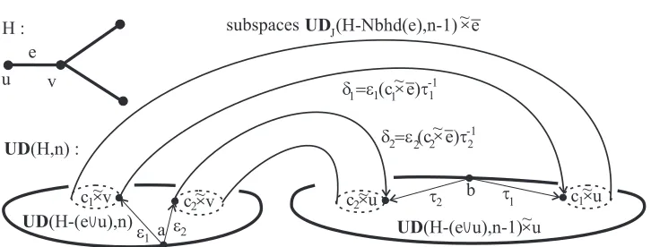
Here one shows how a braid group of a graph changes after adding a hanging edge. In a graph H choose a hanging (open) edge e⊂H attached to a hanging vertex u

and a vertexvof degree at least 3. If the vertexvhas degree degv, thenH−Nbhd(e) consists ofk= degv−1 disjoint subgraphsH1, . . . , Hk. If an edgeej ̸=eattached at

vis also hanging, then the corresponding graphHj is the other endpoint ofej. InUD(H, n) if one robot is ine, then the remainingn₋1 unordered robots from

H₋Nbhd(e) split into k ordered subsets having j1, . . . , jk robots in the subgraphs

of non-negative integer indices such thatj1+· · ·+jk =n−1, let UDJ(H−Nbhd(e), n−1)

be the quotient of

UD(H1, j1)×· · ·×UD(Hk, jk) by the action of the permutation groupSn−1.

UD(H₋Nbhd(e), n₋1) splits into the subspaces UDJ(H₋Nbhd(e), n₋1) over allJ = (j1, . . . , jk) with ordered non-negative integers such thatj1+· · ·+jk =

n−1. Forn= 2, the indexJ degenerates to a single indexj= 1, . . . ,degv−1 of the subgraphHj containing the only remaining robot. Fix base points:

a∈UD(H−(e∪u), n), cJ ∈UDJ(H−Nbhd(e), n−1).

u e

! !

v H :

"#$!#%c e)& "#$!#%c e)&

b

& & c u c u

c v c v

a

UD_{(H-(e u),n) UD}

(H-(e u),n-1) u

UD_{(H,n) :}

UD_{(H-Nbhd(e),n-1) e} J

subspaces

1 2 2 2 1 1 1

-1

-1

2 1

2

2 1

2 1

1 2

~ ~

~

~ _{~ ~} ~

~

Figure 7: Adding a hanging edgeeto a non-hanging vertexv

Figure 7 shows two spaces of the formUDJ(H₋Nbhd(e), n₋1) ˜_×e¯indexed for simplicity by 1 and 2 as in the casen= 2. Fix a point

b_∈UDJ(H₋(e_∪u), n₋1) ˜_×u,

which can be chosen as c1ט u, where c1 is any fixed base point among cJ’s. In

UD(H−Nbhd(e), n−1) find a pathεJfromatocJטv, a pathτJfrombtocJ×u for allJ = (j1, . . . , jk),k= degv−1. The configurationscJט u, cJט vare connected by the motion (cJט ¯e) whenn−1 robots stay fixed atcJ∈UD(H−Nbhd(e), n−1) and one robot moves along ¯e; see Figure 7. AddingεJ,τJ−1at the start and end of the motion (cJט e¯), respectively, one gets the pathsδJ going fromatob inUD(H, n).

Let us make some conventions. For a loopβ_⊂UD(H₋(e_∪u), n₋1) represent-ing a motion of n₋1 robots, the loop (β_{xn=u})⊂UD(H−(e∪u), n−1) ˜×u denotes the motion whenn₋1 robots followβand one robot is fixed atu. The index

nis only a part of the notation (β_{xn=u}) since the robots are not ordered. The subspacesUDJ(H₋Nbhd(e), n₋1) can also be disconnected, at least forn= 2. So π1(UDJ(H−Nbhd(e), n−1)) is interpreted as a formal union of presentations for

the fundamental groups of the connected components fromUDJ(H₋Nbhd(e), n₋

1). For instance, a generator of π1(UDJ(H−Nbhd(e), n−1)) for J= (j1, . . . , jk) means a motion whenj1robots complete a loop in the subgraphH1, otherj2robots

Proposition 3.2(Adding a hanging edgeeto a non-hanging vertexv). In the nota-tions above and for presentanota-tions

π1(UD(H−(e∪u), n)) =⟨α|ρ⟩

and

π1(UD(H−(e∪u), n−1)) =⟨β|λ⟩,

π1(UDJ(H−Nbhd(e), n−1)) =⟨γJ |µJ⟩,

the group π1(UD(H, n)) is generated by α, δ1(β{xn =u})δ−11, δ1δJ−1, subject to

ρ= 1,δ1(λ{xn =u})δ−11= 1,(γJ{xn=v}) =δ1(γJ{xn=u})δ−11.

Proof. By the recursive construction from Lemma 2.6 one has

UD(H, n)_≈UD(H₋e, n)_∪(UD(H₋Nbhd(e), n₋1) ˜_×e¯).

SinceH₋esplits into the vertexuand the remaining subgraphH₋(e_∪u), then the spaceUD(H₋e, n) splits into the subspaces UD(H₋(e_∪u), n), where all robots are inH₋(e_∪u), andUD(H₋(e_∪u), n₋1) ˜_×u, where one robot is atu.

The non-connected subspaceUD(H−Nbhd(e), n−1) ˜×¯esplits into the subspaces UDJ(H−Nbhd(e), n−1) ˜×e¯connecting the subspaces

UD(H−(e∪u), n) and UD(H−(e∪u), n−1) ˜×u.

Indeed, the complement H−Nbhd(e) is obtained from H by removing u, v and all open edges attached to the vertexv of degree degv.

Add the subspaces UDJ(H₋Nbhd(e), n₋1) ˜_×e¯ over all J =_{j1, . . . , jk} to UD(H₋(e_∪u), n). The groupπ1(UD(H−(e∪u), n)) is not affected. Actually, the

added subspaces deformation retract toUDJ(H₋Nbhd(e), n₋1)_×v. This defor-mation is represented by a gradual movement of one robot along ¯etowardsv.

To apply Seifert–van Kampen Theorem 3.1 correctly, add all the pathsδJ to the resulting union above to get the new generatorsδ1δ−J1; see Figure 7. Here 1 denotes one fixed multiple indexJ for simplicity, e.g., 1 = (n₋1,0, . . . ,0).

Consider the spaceUD(H₋(e_∪u), n₋1) ˜_×uas a subspace ofUD(H, n). For-mally a loop β∈π1(UD(H−(e∪u), n−1)) becomes the loop (β{xn=u}) from π1(UD(H−(e∪u), n−1) ˜×u), where one robot remains fixed atu. The same

argu-ment applies to the relatorλ. No other relations appear as the intersection of∪JδJ, andUD(H−(e∪u), n)∪J(UDJ(H−Nbhd(e), n−1) ˜×e¯) contracts toa.

Take the union with the subspace UD(H−(e∪u), n−1) ˜×u. So one adds the generators and relations of π1(UD(H−(e∪u), n−1)) =⟨β|λ⟩. The intersection

deformation retracts to the wedge ofUDJ(H₋Nbhd(e), n₋1) ˜_×uover allJ. Then each generatorγJ gives a relation between the words representing (γJ{xn=v}) in the spacesUD(H₋(e_∪u), n) and UD(H₋(e_∪u), n₋1) ˜_×u. In the latter space the loop can be conjugated byδ1, which replacesb by the pointa∈UD(H, n).

In Proposition 3.2 the loopsδ1(γJ{xn=u})δ1−1 live inUD(H−(e∪u), n) with

the base pointaand can be expressed in terms of the generators δ1(β{xn=u})δ−11.

3.2. Stretching a hanging edge in the unordered case

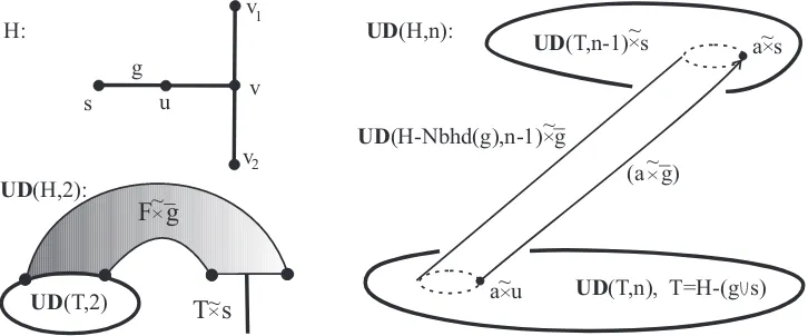
This subsection shows how the presentation of a braid group of a tree changes after stretching a hanging edge of a tree. First consider the degenerate case of stretching a hanging edgeeof the tripod T in the top left picture of Figure 8.

Example 3.3. LetH be the tree obtained by adding a hanging edgeg to the hanging vertexuof the tripodT in the top left picture of Figure 8. Namely,T =H₋(g_∪s), where s is the only hanging vertex of g in the tree H. The complement F =H₋

Nbhd(g) consists of two hanging edges distinct from e and meeting at the centre v

of the tripodT. Let us compute the braid groupB(H,2) by usingB(T,2)∼=Zfrom Example 2.2. By Lemma 2.6 the unordered spaceUD(H,2) has the form

UD(H,2)_≈UD(H₋g,2)_∪(F_ט ¯g)_≈UD(T,2)_∪(T _ט s)_∪(F_ט ¯g).

Here the two components ofUD(H−g,2) are connected by the band Fטg¯. First apply Seifert–van Kampen Theorem 3.1 to the unionUD(T,2)∪(Fטg¯). Then the fundamental group is unchanged, i.e., it is isomorphic to B(T,2)∼=Z. Indeed, the union deformation retracts toUD(T,2). Then apply the same trick taking the union withT_ט s. So one getsB(H,2)∼=Zfor the same reasons.

T s

F g

UD_(H,2):

UD_(T,2) u

a u

(a g)

a s g

v v₁

2 v s

H:

UD_{(T,n), T=H-(g s)} UD_{(T,n-1) s}

UD_(H,n):

UD_{(H-Nbhd(g),n-1) g}

~ _~

~ ~

~ ~

~

Figure 8: Stretching a hanging edge in a treeH

Proposition 3.4 below extends Example 3.3 to a general treeH. Choose an (open) edgeg⊂H with a hanging vertexsand vertexuof degree 2. Fix a base point:

a_∈UD(H₋Nbhd(g), n₋1)_⊂UD(H₋(g_∪s), n₋1).

Denote by (a_ט ¯g) the motion from a_ט u to a_ט s in the space UD(H, n), when

n₋1 robots stay fixed ata, while one robot moves along ¯g; see the right picture of Figure 8. Then, for a loopγ_∈π1(UD(H−Nbhd(g), n−1)), both loops (γ{xn=u}) and (a_ט ¯g)−1_(γ

Proposition 3.4 (Stretching a hanging edge). In the notations above and for pre-sentationsπ1(UD(H−(g∪s), n)) =⟨α|ρ⟩and

π1(UD(H−(g∪s), n−1)) =⟨β|λ⟩, π1(UD(H−Nbhd(g), n−1)) =⟨γ|µ⟩,

π1(UD(H, n))is generated by α, (aט g¯)(β{xn=s})(aט g¯)−1 subject to ρ= 1, (a_ט g¯)(λ_{xn =s})(aט ¯g)−1= 1, (γ{xn=u}) = (aט ¯g)(γ{xn=s})(aט g¯)−1.

Proof. By the recursive construction from Lemma 2.6 one has

UD(H, n)_≈UD(H₋g, n)_∪!UD(H₋Nbhd(g), n₋1) ˜_ׯg".

Here the subspace UD(H₋Nbhd(g), n₋1) ˜_ׯg is glued to UD(H₋g, n) along UD(H₋Nbhd(g), n₋1) ˜_×sandUD(H₋Nbhd(g), n₋1) ˜_×u. Sinceg is hanging, thenH₋Nbhd(g) has the two components: the hanging vertexsand the remaining treeT=H₋(g_∪s), hence UD(H₋g, n)_≈UD(T, n)_∪(UD(T, n₋1) ˜_×s).

Since the edgeeis hanging inH₋(g_∪s) before stretching, then the complement

H₋Nbhd(g) and the space UD(H₋Nbhd(g), n₋1) ˜_ׯg are connected. Adding UD(H₋Nbhd(g), n₋1) ˜_ׯgtoUD(T, n) does not change the presentation. Indeed, the added subspace deformation retracts toUD(H₋Nbhd(g), n₋1) ˜_×u.

AddUD(T, n₋1) ˜_×smeeting the union alongUD(H₋Nbhd(g), n₋1) ˜_×s. By Seifert–van Kampen Theorem 3.1, to get a presentation ofπ1(UD(H, n)) with the

base pointa_טu, one adds the generators (a_ט ¯g)(β_{xn =s})(aט ¯g)−1and relations (a_ט ¯g)(λ_{xn=s})(aט g¯)−1coming from the groupπ1(UD(T, n−1)). Add the new

relations (γ_{xn =u}) = (aט g¯)(γ{xn =s})(aט ¯g)−1 saying that the generators of the group π1(UD(H−Nbhd(g), n−1)) after adding the stationary robot become

homotopic through the subspaceUD(H₋Nbhd(g), n₋1) ˜_×g¯.

3.3. Creating cycles in the unordered case

This subsection extends computations to graphs containing cycles. First let us show how the braid group changes if an edge is added at two vertices of a tripod.

Example 3.5. LetGbe the graph obtained from the tripodT in the top left picture of Figure 9 by adding the edgehat the verticesr, w. By Lemma 2.6 one has

UD(G,2)≈UD(G−h,2)∪!(G−Nbhd(h)) ˜×e¯"≈UD(T,2)∪(¯eט ¯h).

Geometrically the band ¯eט ¯h is glued to the hexagon UD(T,2) as shown in the bottom left picture of Figure 9. To compute the graph braid groupB(G,2), first add to the band ¯eט ¯hthe motionsε,τ⊂UD(T,2) connecting the base configurationuט v

touטr,uטw, respectively. This adds a generator to the trivial fundamental group of the contractible band ¯e_ט ¯_{h. Second, add the union (¯e×}˜_h¯_{)∪(ε∪τ) toUD(T,2),} which gives UD(G,2). The intersection of the spaces attached above has the form (¯e_ט r)_∪(u_ט ¯_h)∪(¯eט w) and is contractible. HenceB(G,2)∼=F2 is the free group

with two generators as the free product ofB(T,2)∼=Zandπ1((¯eט ¯h)∪ε∪τ)∼=Z.

Proposition 3.6 extends Example 3.5 to a general graph excluding the case G_≈ S1_{. Choose an (open) edge h}

e h

e r

e w

b r

b w

UD_(G-h,n) UD_{(G,n) :}

UD_{(G-Nbhd(h),n-1) h}

UD_(G,2):

UD_(T,2) a

(b h)

! !

" "

G :

e r

w v

u _h

~ ~

~ ~ ~

~

~

Figure 9: Adding an edge hcreating cycles

splits into subspacesUDJ(G−Nbhd(h), n−1) indexed byJ = (j1, . . . , jk) with

non-negative integer entries such thatj1+· · ·+jk =n−1; see similar notations before Proposition 3.2. Fixa_∈UD(G₋h, n) andbJ∈UDJ(G−Nbhd(h), n−1).

Denote by (bJט h)⊂UD(G, n) the motion such that one robot goes along the edge h from r to w, while the other robots remain fixed at the base configuration

bJ ∈UDJ(G−Nbhd(h), n−1); see the right picture of Figure 9. In the case k= 1, whenG₋Nbhd(h) is connected, one can skip the indexJ. Take pathsεJ,τJ going from a to bJט r, bJט w, respectively, in UD(G−h, n); see Algorithm 4.3. Then εJ(bJט h)τJ−1is a loop with the base point ain the spaceUD(G, n).

Proposition 3.6 (Adding an edgehcreating cycles).Given the presentations π1(UD(G−h, n)) =⟨α|ρ⟩ and π1(UDJ(G−Nbhd(h), n−1)) =⟨βJ|λJ⟩, the groupπ1(UD(G, n))is generated by α,εJ(bJט h)τJ−1 subject to ρ= 1 and

εJ(βJ{xn=r})ε−_J1= (εJ(bJטh)τ_J−1)·(τJ(βJ{xn =w})τ_J−1)·(εJ(bJט h)τ_J−1)−1. Proof. Each of the subspaces UDJ(G−Nbhd(h), n−1) ˜×h¯ meets the subspace UD(G−h, n) alongUDJ(G−Nbhd(h), n−1) ˜×r,UDJ(G−Nbhd(h), n−1) ˜×w. First add to each subspaceUDJ(G−Nbhd(h), n−1) ˜×h¯ the union of the paths εJ∪τJ as shown in Figure 9, where indicesJ are skipped for simplicity. The funda-mental group of (UDJ(G−Nbhd(h), n−1) ˜×¯h)∪(εJ∪τJ) is isomorphic to the free product ofB(G−Nbhd(h), n−1) and Zgenerated by the loopεJ(bJט h)τJ−1. Sec-ond, add toUD(G₋h, n) each union (UDJ(G₋Nbhd(h), n₋1) ˜_ׯh)_∪(εJ_∪τJ). The intersection of the spaces attached above is the union over allJ of the subspaces

!

UDJ(G−Nbhd(h), n−1) ˜×r"∪(εJ∪τJ)∪!UDJ(G−Nbhd(h), n−1) ˜×w".

Each space above is homotopically a wedge of two copies ofUDJ(G−Nbhd(h), n− 1). By Seifert–van Kampen Theorem 3.1, express the loopsεJ(βJ{xn =r})ε−_J1 and τJ(βJ{xn=w})τJ−1generating the fundamental group of the intersection in terms of the loops fromUD(G−h, n) and (UDJ(G−Nbhd(h), n−1) ˜×¯h)∪(εJ∪τJ). In the latter space these loops are conjugated byεJ(bJט h)τJ−1as required, i.e., homotopic through the subspaceUDJ(G−Nbhd(h), n−1) ˜×¯h.

If the vectorβis empty, i.e., the groupsπ1(UDJ(G−Nbhd(h), n−1)) are trivial,

4.

Computing graph braid groups

Step-by-step instructions of Algorithm 1.5 are based on the technical propositions from Section 3 and the auxiliary algorithms from Subsection 4.1. Proposition 4.8 extends the result about 2-point braid groups of graphs with only disjoint cycles [6, Theorem 5.6] to a wider class of graphs including all light planar graphs.

4.1. A motion planning algorithm in the unordered case

Proposition 3.2 requires a collision free motion connecting two configurations ofn

robots. Take a connected graphGand number its vertices. Let us work with discrete configuration spaces assuming that at every discrete time moment all robots are at vertices of a graphG. So in one step any robot can move to an adjacent vertex if it is not occupied. The output contains positions of all robots at every moment.

To describe planning Algorithm 4.3 introduce auxiliary definitions and searching Algorithms 4.1 and 4.2. A robot xi∈G is called extreme in a given configuration (x1, . . . , xn)∈OD(G, n) if the remaining robots are in one connected component of

G_−{xi}. One configuration may have several extreme robots, e.g., on a segment there are always two extreme robots, while on a circle every robot is extreme.

Algorithm 4.1. If a graph Ghasl edges, then there is an algorithm of complexity

O(nl) to find an extreme robot in a configuration (x1, . . . , xn)∈OD(G, n).

Proof. For a robot xi, visit all vertices from a connected component of G−{xi} remembering the robots that were seen. If not all robots were seen, then xi is not extreme, so choose a robot xj that was visited in a component of G−{xi}. If xj is extreme among the robots in the closure of this componentG_−{xi}, then xj is extreme in the given configuration (x1, . . . , xn)∈OD(G, n). Hence one inevitably

finds an extreme robot, which requires not more thanl steps for any candidate.

A robot xj is a neighbour of a robot xi if a shortest path from xi to xj has the minimal number of edges among all shortest paths fromxi to robotsxk fork̸=i. For

nrobots on a segment each of the two extreme robots has a unique neighbour, while on a circle each robot has two neighbours. A shortest path to a neighbour does not contain other robots, i.e., the corresponding motion is collision free.

Algorithm 4.2. If a connected graph Ghas l edges, then there is an algorithm of complexityO(l) to find a shortest path from a robotxi to one of its neighbourxj in a given configuration of unordered robots (x1, . . . , xn)∈UD(G, n).

Proof. One travels on Gin a ‘spiral’ way starting from xi. So first visit all vertices adjacent toxi and check if there is another robot xj at one of them, which can be a neighbour of xi. If not, then repeat the same procedure recursively for all these adjacent vertices. In total, one passes through not more thanl edges ofG.

Algorithm 4.3. If a connected graph Ghas l edges, then there is an algorithm of complexityO(n2_{(l+n)) that, given any two configurations ofnunordered robots in}

G, finds a path in the space UD(G, n) between the given configurations.

increases the numberl of edges by not more than nto l+n. The initial (and final) configuration of robots is considered as an array of vertices where thenrobots are located. During each elementary move, only one robot goes to an adjacent vertex. The resulting configuration is represented by a new array of positions.

Step 1.Using Algorithm 4.1 of complexityO(n(l+n)), find an extreme robot in the collection of 2ngiven positions (initial and final together) ordered arbitrarily.

Step 2.Assume that the found extreme robot, sayyn, is from the final configura-tion, otherwise swap the roles of initial and final positions. Using Algorithm 4.2 of complexityO(l+n), find a shortest path fromyn to its neighbour, sayxn, from the initial configuration. Then safely movexntowardsyn along the shortest path without any collisions and keeping fixed all other robots from the initial configuration.

Step 3.In the graph Gremove the robot yn located at a vertex of degree 2 and all open edges attached toyn. This removal reduces the problem to a smaller graph withn−1 robots. The new graph remains connected since the robotynwas extreme. Return to Step 1 and apply the recursion n−1 times, which gives O(n2_(l+n))

operations.

In Algorithm 4.3 the quadratic complexity in the number of robots seems to be asymptotically optimal, because avoiding collisions betweennrobots should involve some analysis of their pairwise positions. Another quadratic algorithm for checking the non-trivial topological property of basic embeddability of any finite graphs into a product of small graphs was designed in [10]. One more algorithm of linear complexity was found to verify whether a combinatorial code (a Gauss paragraph of several words) encodes a classical link in 3-space [11]. Finally, Algorithm 1.5 is deterministic up to ordering edges ofGand choosing an extreme robot at every stage.

Step-by-step instructions of Algorithm 1.5

Step 1.To write down a presentation of the group B(G, n) for an arbitrary con-nected graph G, start from from nrobots on a segment subdivided into n₋1 sub-segments. Then the configuration spaceUD([0,1], n) is a single point, soB([0,1], n) is trivial.

Step 2.Fix a plan to construct the given graphGby adding edges to [0,1]. Step 3.If a hanging edge is added to a vertex of degree at least 2, then follow the rules of Proposition 3.2 to update the presentation of the braid group of the already constructed graph. If one needs a motion to connect two configurations ofnrobots, then follow the steps of motion planning Algorithm 4.3.

Step 4.If a hanging edge is added to a vertex of degree 1, then follow the rules of Proposition 3.4 to update the presentation of the current graph braid group.

Step 5.If one adds an edge that creates a new cycle, then apply Proposition 3.6. Every generator in the resulting group presentation is encoded by a list of successive configurations that show where the robots are located at every discrete moment.

4.2. Two-point braid groups of graphs in the unordered case

Lemma 4.4. For any tree H, the braid group B(H,2) is free and has the rank %

(degv−1)(degv−2)/2, where the sum is over all vertices of degree at least3.

Proof. Induction on the number of edges ofH. The baseH _≈[0,1] is trivial. In the inductive step notice that trees are contractible. Hence their fundamental groups are trivial and forn= 2 the vectorsβ,γ,λ,µ(with indices) are empty in Propositions 3.2 and 3.4. The vectorsρare also empty, because they can only come from 2-point braid groups of smaller trees. So the braid group B(H,2) is free. In the case n= 2 the multiple indexJ in Proposition 3.2 degenerates to a single indexj= 1, . . . ,degv₋1. Then the only generators ofB(H,2) areδ1δj−1,j= 2, . . . ,degv−1. In total, one gets

1 + 2 +_{· · ·}+ (degv₋2) = (degv₋1)(degv₋2)/2 generators after attaching all edges to each vertexv of degree degv.

The Kuratowski graphs K5, K3,3 in Figure 2 do not satisfy Lemma 4.5. Indeed,

the complement to the neighbourhood of any edgeh_∈K5(h∈K3,3, respectively) is

the triangular (rectangular, respectively) cycle intersecting any cycleC_⊃h.

Lemma 4.5. Any light planar graph can be constructed from a tree by adding edges as follows: an open edge hadded to the new graphG creates a cycle C not meeting any cycle fromG−Nbhd(h)having all its cycles in one connected component. Proof. A planar connected graph Gis light if any cycle C_⊂G has an edgeh such that all cycles fromG₋¯h(or, equivalently,G₋Nbhd(h)) do not meetC. For a given light planar graphG, take any cycleC and the corresponding edgeh. The subgraph

G−his light planar, becauseG−hhas fewer cycles satisfying the same condition.

G-Nbhd(h)

h

C

Figure 10: Choosing an edge hand a cycle C_⊃hin Lemma 4.5

One can assume that all cycles of the subgraphG₋Nbhd(h) are in one connected component. Otherwise, choose another cycle from a component ofG₋Nbhd(h) with a smaller number of edges; see the left-hand side picture of Figure 10, and so on until one finds a cycle with an edge h such that G₋Nbhd(h) has all its cycles in one component. Remove edges one-by-one until the graph becomes a tree. Then the original graphGcan be reconstructed by reversing the procedure above.

implies that Corollary 1.6 for unordered robots is a particular case of more technical Proposition 4.8, which holds for all graphs constructed as described above.

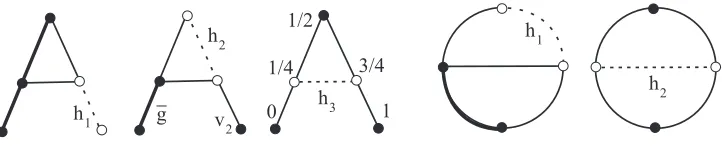
Corollary 4.6.The A-graph in the left-hand side picture of Figure 11 below has the braid groupB(A,2)∼=F3, the free group with three generators.

Proof. Three proofs are given below to illustrate different approaches.

1. The A-graph is obtained from the graph Gin the top left picture of Figure 9 in Example 3.5 by adding the hanging edge h1 to the vertex w of degree 2.

The complement A−Nbhd(h1)≈[0,1] is connected. Hence one can skip the

multiple indexJand apply Proposition 3.2 to the free groupB(G,2)∼=F2. One

adds no relations and one generator δ1δ−21 since degw= 3 in the A-graph, so

B(A,2)∼=F3.

2. The sameA-graph can also be obtained by adding the open edgeh2to the graph

H in the top left picture of Figure 8; see Example 3.3. One of the endpoints of

h2 is the vertexu∈H of degree 2, and the other one is the hanging vertexv1.

Apply Proposition 3.6 to computeB(A,2) fromB(H,2)∼=Z. The complement

A−Nbhd(h2) is not connected and consists of the closed hanging edge ¯g and

the remaining hanging vertexv2∈H. Then the multiple indexJ takes only two

values (1,0) and (0,1) in Proposition 3.6, i.e., one adds no relations and two new generators of the form εJ(b_ט h)τ_J−1 to B(H,2)∼=Z. Hence one gets the free group B(A,2)∼=F3 as expected.

3. Finally the A-graph can be obtained from the segment [0,1] with vertices 0, 1/4, 1/2, 3/4, 1 by adding an open edgeh3 at 1/4, 3/4. Then the complement

A−Nbhd(h3) consists of three vertices 0,1/2,1∈[0,1]. Hence Proposition 3.6

adds three generators without relations to the groupB([0,1],2) = 1, i.e.,B(A,2) ∼

=F3.

Figure 11: Choosing different edges in theA-graph and θ-graph

Corollary 4.7.Theθ-graph in the right-hand side picture of Figure 11 above has the braid groupB(θ,2)∼=F3, the free group with three generators.

Proof. Two proofs are given below to illustrate different approaches:

1. The θ-graph is obtained from the graphG in the top left-hand side picture of Figure 9 in Example 3.5 by adding an open edge h1 connecting the vertices

u, w_∈G. ComputeB(θ,2) from B(G,2)∼=F2 by using Proposition 3.6. Then

θ₋Nbhd(h1) is a single edge. No relations and one generator are added, so one

2. The θ-graph can also be obtained from a circle S1 _{with two pairs of opposite}

vertices by adding an open horizontal diameter h2 at one of these pairs. Then

the complement θ−Nbhd(h2) is the other pair of the opposite vertices. Hence

the multiple index J in Proposition 3.6 takes only two values (1,0) and (0,1). This adds no relations and two generators toB(S1_,2)∼_{=Z, i.e.,B(θ,2)}∼_=F

3as

expected.

Corollaries 4.6 and 4.7 agree with [9, Example 2.1] and [6, Example 5.2], respec-tively, based on the discrete Morse theory. The following result extends these com-putations to a wider class of graphs including all light planar graphs:

Proposition 4.8. Let a graph G be constructed from a tree T as in Lemma 4.5 by adding open edgesh1, . . . , hm, i.e.,G1=T∪h1,G2=G1∪h2, . . . , G=Gm−1∪hm.

Letkj be the number of connected components of Gj−Nbhd(hj), whereGm=G. The braid groupB(G,2) has a presentation with

m &

j=1

kj+ &

(degv₋1)(degv₋2)/2

generators subject to commutator relations, where the second sum is over all vertices

v∈T of degree at least3 in the treeT. A geometric description follows:

1. At each vertex v_∈G fix an edge e0. For any unordered pair of other edges

ei, ej at the same vertexv,j= 1, . . . ,degv−1, one generator ofB(G,2)swaps two robots in the tripod e0∪ei∪ej by using the collision free motion shown in Figure 1.

2. The remaining%m_j=1kj generators ofB(G,2)represent motions when one robot remains in a connected component ofGj−Nbhd(hj), and the other robot moves without collisions along a cycle ˆhj containing the open edge hj chosen above. 3. Each relation says that motions of two robots along disjoint cycles commute. Proof. Computing the 2-point braid group B(G,2) by Subdivision Theorem 1.4, assume that G has no loops and multiple edges after removing extra trivial ver-tices of degree 2. Induction on the first Betti numberm. Basem= 0 is Lemma 4.4, where every generator δ1δj−1 coming from Proposition 3.2 is represented by a loop that swaps two robots near a vertex of degree at least 3 as shown in Figure 1.

In the inductive step fromm₋1 tom, for an open edgeh_⊂Gfrom Lemma 4.5, let us show how a presentation ofB(G,2) differs from a presentation ofB(G₋h,2) satisfying the conditions by the inductive hypothesis. Proposition 3.6 adds motions such that one of the two robots moves along the newly added edgeh, while the other robot remains in a connected component ofG₋Nbhd(h), whose index is encoded by the place of 1 in thekm-tuple index J of the form (0, . . . ,0,1,0. . . ,0).

The relationsλJ are trivial sincen= 2 and fundamental groups of graphs are free. By Lemma 4.5 the complementG₋Nbhd(h) has all its cycles in one connected com-ponent. Hence the generatorsβJ of π1(UDJ(G−Nbhd(h),1)) are non-trivial only

It remains to show that the loops (βJ{x2=r}) and (βJ{x2=w}) are homotopic,

i.e., the new relator is a commutator. Take the cycle C⊃h from the construction of Lemma 4.5. Since C does not meet all cycles from G−Nbhd(h), then one can move one robot along C−hfrom r to w without collisions with the other robot is moving along the loopsβJ. These loops generate the fundamental group of the single non-contractible component ofG−Nbhd(h). One gets a free homotopy from

(βJ{x2=r}) to (βJ{x2=w}) = (bJט (C−h))·(βJ{x2=r})·(bJט (C−h))−1. During the motion (bJט (C−h)), one robot is fixed at bJ ∈G−Nbhd(h), while the other moves alongC−havoiding all cycles of G−Nbhd(h). In Proposition 3.6 choose the pathτJfromatobJט winUD(G−h,2) so thatτJ=εJ·(bJט (C−h)). Then the loops εJ(β{x2=r})ε−J1 and τJ(βJ{x2=w})τJ−1 are homotopic with the fixed base configurationa∈UD(G−h,2).

The following result agrees with [6, Example 5.4]:

Corollary 4.9.The ⊕-graph in the left-hand side picture of Figure 12 below has the braid groupB(_⊕,2)∼=F5, the free group with five generators.

Proof. The open edgeh0⊂ ⊕can not appear in the construction of Lemma 4.5 since

all cycles of_⊕throughh0 meet the triangle⊕ −Nbhd(h0) at the central vertex.

The vertical radius h1 is allowed by Lemma 4.5 since ⊕ −Nbhd(h1)≈[0,1] is

the lower half-circle. Then Proposition 3.6 implies thatB(_⊕,2) is the free product of _Z and B(_{⊕ −}h1,2). Applying Lemma 4.5 to the subgraph ⊕ −h1, choose the

remaining vertical radiush2such that (⊕ −h1)−Nbhd(h2)≈[0,1] is the upper

half-circle. By Proposition 3.6 the group B(_{⊕ −}h1,2) is the free product ofZ and the

groupB(_{⊕ −}(h1∪h2),2) =B(θ,2)∼=F3by Corollary 4.7, henceB(⊕,2)∼=F5.

h v h

h v b c

p q

h

h

h v

h _v

1 1

1

4 4 0

2

2 2

3 ₃

Figure 12: Choosing different edges in the⊕-graph and tree with balloons

Corollary 4.10. The graph G in the right-hand side picture of Figure 12 has the braid groupB(G,2) that has a presentation with 11generators and six commutator relations.

Proof. The graphGhas four loopsf1, f2, f3, f4 attached at the verticesv1, v2, v3, v4,

respectively. ComputingB(G,2) by Theorem 1.4, one can subdivide each simple loop

fj into three subedges. Denote by hj⊂fj the middle subedge not containing vj. ThenG₋Nbhd(hj) is obtained fromGby removing the simple loopfj, but keeping

vj. The groupB(G,2) will be computed by removing the open edgeshj.

By Lemma 4.4 for T =G₋(h1∪h2∪h2∪h3), the group B(T,2) is free and is

of degree 3 in T. Let ε1 be the natural path from the base configuration bט c to

b_ט v1. Before applying Proposition 3.6, gradually move the endpoints of h1 to the

adjacent vertexv1, then the pathτ1 coincides with ε1. Attaching the open edge h1

adds no relations and the generatore1=ε1(bט f1)ε−11representing the motion when

one robot stays atb, while the other robot goes aroundf1. Attaching the next open

edgeh2adds the similar generatore2=ε2(bט f2)ε−21and one relation saying thate2

commutes withε2(f1{x2=v2})ε2−1, whereε2is the natural path frombט ctobט v2.

Geometrically, the last loop is conjugated toe1by the motions(c) swapping the robots

aroundc, i.e., the robots go aroundf1, f2without collisions: [e2, s(c)e1s(c)−1] = 1.

Attaching h3, h4 similarly adds the generators e3, e4 and [e3, s(c)e1s(c)−1] = 1,

[e3, s(p)e2s(p)−1] = [e4, s(q)e1s(q)−1] = [e4, s(c)e2s(c)−1] = [e4, s(c)e3s(c)−1] = 1.

Corollaries 4.9 and 4.10 show that Proposition 4.8 and general Algorithm 1.5 effec-tively compute braid groups of graphs by using known results without starting from scratch. Generalising Sections 3 and 4 to the case of ordered robots is left to the reader.

References

[1] A. Abrams, Configuration spaces and braid groups of graphs, Ph.D. the-sis, 2000, UC Berkeley, available at http://www.math.uga.edu/∼abrams/ research.

[2] C. Adams and R. Franzosa,Introduction to topology: pure and applied, Pearson Prentice Hall, Upper Saddle River, NJ, 2008.

[3] R. Crowell and R. Fox,Introduction to knot theory, Springer-Verlag, New York, 1963.

[4] M. Farber, Collision free motion planning on graphs, inAlgorithmic foundations of robotics VI, Utrecht/Zeist, 2004, MPIM2004-87.

[5] D. Farley and L. Sabalka, Discrete Morse theory and graph braid groups, Alge-braic and Geometric Topology 5(2005), 1075–1109.

[6] D. Farley and L. Sabalka, Presentations of graph braid groups, arXiv: 0907.2730

[7] R. Forman, Morse theory for cell complexes, Adv. Math. 134 (1998), no. 1, 90–145.

[8] R. Ghrist, Configuration spaces and braid groups on graphs in robotics, in Knots, braids, and mapping class groups—papers dedicated to Joan S. Birman (New York, 1988), AMS/IP Stud. Adv. Math.24 (2000) 29–40, AMS, Provi-dence, RI, 29–40.

[9] J.H. Kim, K.H. Ko and H.W. Park, Graph braid groups and right-angled Artin groups,Trans. Amer. Math. Soc.364(2012), no. 1, 309–360.

[10] V. Kurlin, Basic embeddings into a product of graphs, Topology Appl. 102 (2000), no. 2, 113–137.

[12] P. Prue and T. Scrimshaw, Abrams’s stable equivalence for graph braid groups,

arXiv:0909.5511.

Vitaliy Kurlin vitaliy.kurlin@durham.ac.uk