This is a repository copy of
The distribution of species range size: a stochastic process
.
White Rose Research Online URL for this paper:
http://eprints.whiterose.ac.uk/1342/
Article:
Gaston, K.J. and He, F. (2002) The distribution of species range size: a stochastic process.
Proceedings of the Royal Society B: Biological Sciences, 269 (1495). pp. 1079-1086. ISSN
1471-2954
DOI:10.1098/rspb.2002.1969
[email protected] https://eprints.whiterose.ac.uk/ Reuse
Unless indicated otherwise, fulltext items are protected by copyright with all rights reserved. The copyright exception in section 29 of the Copyright, Designs and Patents Act 1988 allows the making of a single copy solely for the purpose of non-commercial research or private study within the limits of fair dealing. The publisher or other rights-holder may allow further reproduction and re-use of this version - refer to the White Rose Research Online record for this item. Where records identify the publisher as the copyright holder, users can verify any specific terms of use on the publisher’s website.
Takedown
If you consider content in White Rose Research Online to be in breach of UK law, please notify us by
Published online1 May 2002
The distribution of species range size:
a stochastic process
Kevin J. Gaston
1*and Fangliang He
2,31Biodiversity and Macroecology Group, Department of Animal and Plant Sciences, University of Sheffield, Sheffield S10 2TN, UK
2Canadian Forest Service, Pacific Forestry Centre, Victoria, BC, Canada V8Z 1M5
3Department of Statistics and Actuarial Science, Simon Fraser University, 8888 University Drive, Burnaby, BC, Canada V5A 1S6
The major role played by environmental factors in determining the geographical range sizes of species raises the possibility of describing their long-term dynamics in relatively simple terms, a goal which has hitherto proved elusive. Here we develop a stochastic differential equation to describe the dynamics of the range size of an individual species based on the relationship between abundance and range size, derive a limiting stationary probability model to quantify the stochastic nature of the range size for that species at steady state, and then generalize this model to the species-range size distribution for an assemblage. The model fits well to several empirical datasets of the geographical range sizes of species in taxonomic assemblages, and provides the simplest explanation of species-range size distributions to date.
Keywords:geographical range size; macroecology; stochasticity; temporal dynamics
1. INTRODUCTION
Species differ enormously in the sizes of their geographical ranges. Some are narrowly distributed, and others occur over areas that may be many orders of magnitude larger
(Brownet al.1996; Gaston 1996). For a given taxonomic
assemblage, the frequency distribution of species range sizes (the species-range size distribution) tends to be strongly right-skewed, with the smallest size class being the modal one. That is, most species are rather restricted in their geographical occurrence, and only a few are
wide-spread (Anderson 1977, 1984a,b; Pagelet al.1991;
Gas-ton 1994, 1996, 1998; Brown et al. 1996; Gaston &
Chown 1999).
Much of the discussion of the determinants of the shape of species-range size distributions has focused on the roles of speciation and extinction processes (e.g. Anderson 1985; Flessa & Thomas 1985; Chown 1997; Gaston 1998; Gaston & Chown 1999). Speciation adds new ranges and, depending on its mode, may reduce the sizes of those of the ancestral species (e.g. through vicariance). Extinction removes ranges. Although they clearly deter-mine the number of species that are extant at any one time, it is unlikely, however, that these processes are suf-ficient themselves to explain the species-range size distri-butions that are actually observed. Rather, the form of these distributions will be set principally by the temporal dynamics (expansions and contractions) of the range sizes of species between their first appearance and their ultimate demise (Webb & Gaston 2000). These dynamics in turn will be determined by the environmental tolerances and capacities of species (and the effects of selection on these features), how abiotic and biotic conditions change, and how species are able to respond to these changes (e.g. dis-persal and colonization abilities). Indeed, the influence of
*Author for correspendence ([email protected]).
Proc. R. Soc. Lond.B (2002)269, 1079–1086 1079 2002 The Royal Society
environmental changes on geographical ranges is well established, with local populations being founded and lost, and range limits moving as conditions alter in ecological, let alone evolutionary, time (Burton 1995, 2001; Spicer & Gaston 1999; Dynesius & Jansson 2000; Hewitt 2000).
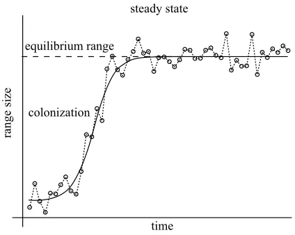
The importance of environmental factors, and the ability of species to respond, in influencing geographical range sizes raises the possibility of developing a stochastic theory of species-range size distributions. At any one time, the majority of species will have passed beyond the strongly determinate phase of range expansion associated with their initial geographical spread, and the colonization of, and establishment in, new habitats (figure 1). Sub-sequent changes in range size will reflect both non-random and random temporal variations in the environment. The consequences of both are, however, difficult to predict. Even non-random environmental changes may have com-plex effects because these changes are themselves spatially heterogeneous and temporally complex (with cycles com-monly acting on several time-scales in addition to any broader directional trends), and because for any given species the individuals on which they are acting commonly exhibit both phenotypic and genotypic variation, and thus different responses to a particular alteration of conditions (Spicer & Gaston 1999). Thus, even when local popu-lation dynamics and shifts of particular range boundaries may be interpretable in terms of local conditions, changes in the size of whole ranges may often appear essentially stochastic (see § 5).
1080 K. J. Gaston and F. He Distribution of species range sizes
range size
time equilibrium range
steady state
[image:3.598.65.277.62.231.2]colonization
Figure 1. Dynamics of range size. The dashed curve shows the stochastic dynamics of the range size of a species, whereas the smooth solid curve shows the deterministic growth. At a certain point, the range reaches a dynamic equilibrium about which its size fluctuates.
from one species to another. The model is finally tested using several empirical datasets of the geographical range sizes of species in taxonomic assemblages.
2. MODEL
(a) SDE of range size
Let x(t) be the abundance of a population at time t.
The dynamics of x(t) are traditionally modelled with an
ordinary differential equation, such as the logistic growth model,
dx(t)=rx(t)
冉
1⫺x(t)k
冊
dt, (2.1)wherer is the specific growth rate and k is the
environ-mental carrying capacity supporting the population at
x(⬁), i.e. the population approacheskas t→ ⬁.
In reality, populations seldom grow in a deterministic manner, but rather in a stochastic one. An approach to modelling stochastic growth is to view the specific growth
rateras being subject to stochastic environmental
fluctu-ations, which is equivalent to adding a white noise term to equation (2.1) (e.g. May 1974),
dx(t)=rx(t)
冉
1⫺x(t)k
冊
dt⫹x(t)dw(t), (2.2)where dw(t) is Gaussian white noise withN(0,dt). Here,
at steady state (i.e. as t → ⬁) the population fluctuates
along the deterministic equilibriumk. This gives rise to a
gamma probability distribution for the population
(Dennis & Costantino 1988).
The relationship between the abundance x(t) and the
range sizey(t) of a species can be expressed in terms of a
power model (Gaston 1994; Leitner & Rosenzweig 1997;
Harteet al.2001),
y(t)=ax(t)b, (2.3)
wherea and bare parameters. Both abundance x(t) and
range size y(t) are random variables and dependent on
time in equation (2.3). The SDE fory(t) can therefore be
Proc. R. Soc. Lond.B (2002)
derived according to the following transformation
(transformingx(t) toy(t)) for the Ito stochastic differential
(Karlin & Taylor 1981, p. 347)
dy(t)=
冋
∂y(t)∂x(t)rx(t)
冉
1⫺ x(t)k
冊
⫹ ∂y(t)∂t
⫹1
2 ∂2y(t) ∂x(t)2
2x(t)2
册
dt⫹∂y(t)∂x(t)x(t)dw(t). (2.4)
Substituting the appropriate derivatives of equation
(2.3) and further replacing dx(t)/dtby equation (2.2), we
arrive at an SDE for range size,
dy(t)=y(t)
冋
4r⫹(1⫺)2
22 ⫺
2r␣
k y(t)

册
dt⫹2
y(t)dw(t), (2.5)
where, in terms of the parameters in equation (2.3),
␣=
冉
1a
冊
1 band =1
b.
This SDE (equation (2.5)) describes the stochastic dynamics of the range size of a species, and is of the logis-tic type, with a trajectory as shown in figure 1.
(b) Steady-state probabilistic distribution of range size
If=0, the SDE (equation (2.5)) becomes a
determin-istic differential equation. When time is sufficient, the
range sizey(t) of a species will reach a stable equilibrium
(figure 1),y(⬁)=(k/␣)1/. In the stochastic setting, ⬎
0, the range size of the species fluctuates above and below this equilibrium. Therefore, at the steady state, the range size approaches an approximately limiting, stationary pro-babilistic distribution of the form
f(y)=exp
冋
22
冕
g(y)
y dx⫺2log(y)
册
, y⬎0, (2.6)for an SDE dy=yg(y)dt⫹ydw(t) (see Dennis &
Costan-tino 1988). is a constant that makes equation (2.6) a
probability density function (PDF), i.e. the integration of
f(y) over the support ofyequals 1.
Applying equation (2.6) to the SDE of equation (2.5),
results in the stationary PDF for range sizey
f(y)=y
r
2 ⫺
4⫺ 7
4exp
冉
⫺ ␣r2ky

冊
, 0⬍y⬍ ⬁. (2.7)Solving for constantby setting the integration of
equa-tion (2.7) over 0⬍y⬍ ⬁to be 1, we obtain a stationary
distribution for the range sizeyof a species that is a
gen-eralized gamma distribution
f(y)=

冉
ck
冊
␦
⌫(␦)y
␦⫺1exp
冉
⫺c ky
冊
, y⬎0, (2.8)where␦= r
2⫺
3
4⫺
1
4andc=
␣r
2.
The PDF (equation (2.8)) describes the steady-state distribution of range size for a species that fluctuates above
and below the equilibrium range (figure 1). ␦ and are
the two parameters determining the shape of the
5
4
3
2
1
0
1.0 0.8 0.6 0.4 0.2 0
5
4
3
2
1
0
1.0 0.8 0.6 0.4 0.2 0
5
4
3
2
1
0
1.0 0.8 0.6 0.4 0.2 0 10
8
6
4
2
0
1.0 0.8 0.6 0.4 0.2 0
1/range size 1/range size
(a)
(c)
(b)
probability density
[image:4.598.122.481.63.397.2](d)
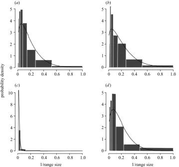
Figure 2. The probability densities for the inverse range sizes of species to illustrate the validity of the exponential assumption for equation (2.9). The smooth curves are the fittings of the Weibull distribution to the inverse of range sizes for four assemblages: (a) bumble-bees; (b) New World birds (overall); (c) primates; (d) woodpeckers. See § 4 for descriptions of the datasets.
decreasing to unimodal when ␦ (or ) varies from small
to large. On the other hand,c/k is a position parameter.
A smallk (the carrying capacity) (or a largec) leads the
distribution to be concentrated in the small range classes,
whereas a largekmakes the distribution more evenly
dis-tributed from small to large range classes. If there were time-series of measurements of the range size of a species, the data would be expected to follow this distribution. Unfortunately, such data are not available.
There is variation between species in the growth rate of range size, reflecting differences in their population growth rates. This variation has been accounted for in the SDE (2.2) through the stochastic term, and thus in equ-ation (2.5). If all species had the same equilibrium range size, equation (2.8) would be sufficient to describe the dis-tribution of range sizes for a species assemblage. However, in reality, there is also variation between species in the equilibrium range size, resulting from differences in
equi-librium populationk. Variation in equilibrium range size
can be accounted for by considering the carrying capacity
kin equation (2.8) to be a random variable. To simplify,
here we assume the inverse of kto follow an exponential
distribution
f
冉
z=1k
冊
=exp(⫺z), z⬎0. (2.9)This assumption is simple yet not unreasonable. This
can be approximately corroborated because if we assume that the observed range size of each species had indeed reached the deterministic equilibrium, the inverse of these
range sizes (i.e. 1/y) would be expected to follow the
Wei-bull distribution. The WeiWei-bull distribution is derived through variable transformation according to equation
(2.3) at x(t)=k. We have found this to be the case for
several datasets (including those employed below; see figure 2), probably reflecting the pattern of resource par-titioning among the species in an assemblage (see § 5).
A compound distribution of equation (2.8) can be con-structed by assuming the exponential distribution of
equ-ation (2.9) for 1/k
f(y)= c
␦
⌫(␦)y
␦⫺1
冕
⬁
0
z␦exp(⫺cyz)exp(⫺z)dz. (2.10)
The integration in equation (2.10) leads to the distri-bution
f(y)=␦ y
␦⫺1
( ⫹y)␦⫹1, y⬎0 (2.11)
where=/c. This is the PDF of a Pearson type VI
1082 K. J. Gaston and F. He Distribution of species range sizes
0.08
0.06
0.04
0.02
0
500 400 300 200 100 0
y
0.4
0.3
0.2
0.1
0
6 6 6 6 6 6 6 6 6 6 6 6 5 4 3 2 1
log (y)
probability density
probability density
[image:5.598.115.481.61.257.2](a) (b)
Figure 3. Shapes of the probability model (equation (2.11)) for five numerical examples. (a) The probability density functions for the original data (solid line,= 1.0,␦=0.5,=1000; dotted line,=1.0,␦=0.5,=20; long dashes,=1.0,␦ =1.0,=20; dot and dashed line, =1.0,␦=1.0,=100; dashed line,=1.5,␦=1.5,=20). The curves are strongly
right-skewed, except in the fifth case (dashed line) which has a mode aty =5. (b) The corresponding densities for the log-transformed data.
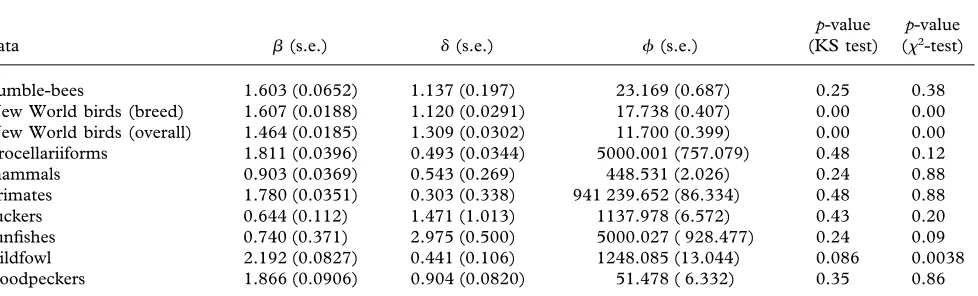
Table 1. The maximum-likelihood estimates of the parameters of equation (2.11) (±s.e.) and the results of KS and2
goodness-of-fit tests to 10 range size datasets.
p-value p-value
data (s.e.) ␦(s.e.) (s.e.) (KS test) (2-test)
bumble-bees 1.603 (0.0652) 1.137 (0.197) 23.169 (0.687) 0.25 0.38 New World birds (breed) 1.607 (0.0188) 1.120 (0.0291) 17.738 (0.407) 0.00 0.00 New World birds (overall) 1.464 (0.0185) 1.309 (0.0302) 11.700 (0.399) 0.00 0.00 Procellariiforms 1.811 (0.0396) 0.493 (0.0344) 5000.001 (757.079) 0.48 0.12 mammals 0.903 (0.0369) 0.543 (0.269) 448.531 (2.026) 0.24 0.88 primates 1.780 (0.0351) 0.303 (0.338) 941 239.652 (86.334) 0.48 0.88 suckers 0.644 (0.112) 1.471 (1.013) 1137.978 (6.572) 0.43 0.20 sunfishes 0.740 (0.371) 2.975 (0.500) 5000.027 ( 928.477) 0.24 0.09 wildfowl 2.192 (0.0827) 0.441 (0.106) 1248.085 (13.044) 0.086 0.0038 woodpeckers 1.866 (0.0906) 0.904 (0.0820) 51.478 ( 6.332) 0.35 0.86
show a mode at very small range sizes and be strongly skewed to the right (figure 3).
3. PARAMETER ESTIMATION AND GOODNESS-OF-FIT
The maximum-likelihood estimates of the parameters of equation (2.11) are easy to compute. Given observed
range sizes fornspeciesy={y1,y2,…yn}, the joint PDF
of equation (2.11) isf(y). The log-likelihood function of
equation (2.11) is
l(,␦,;y)=
冘
n
i=1
log(f(y)). (3.1)
The maximum-likelihood estimates of the three
para-meters (,␦,) are obtained by maximizing the
log-likeli-hood function (equation (3.1)). The maximization of the likelihood function is evaluated using the iterative New-ton–Raphson method, and the Hessian matrix used in the Newton–Raphson method (constructed from the second-order derivatives of the log-likelihood function) is used to derive the asymptotic standard errors for the estimates.
Proc. R. Soc. Lond.B (2002)
The goodness-of-fit of the model to the observed range data is tested using both the Kolmogorov–Smirnov (KS)
test and the2-test. The null hypothesis is: does the
sam-ple arise from the hypothesized distribution (equation (2.11))? For continuous data, the KS test is generally
more powerful than the2-test and is more likely to reject
the null hypothesis.
4. EMPIRICAL EVALUATION OF THE STOCHASTIC MODEL
(a) Data
We have acquired geographical range size data for 10 assemblages of species covering a wide range of taxonomic groups (details of the varied methods employed for the calculation of range sizes are provided in the references cited): (i) bumble-bees—global overall range sizes of 241 species (P. H. Williams, unpublished data; Gaston 1996); (ii) New World birds—breeding range sizes for 3901 spec-ies (Blackburn & Gaston 1996); (iii) New World birds— overall range sizes for 3906 species (Blackburn & Gaston 1996); (iv) Procellariiform seabirds—global overall range
[image:5.598.58.547.358.506.2]0.4 0.3 0.2 0.1 0 5 4 3 2 1 0 log (bumble-bee) 0.4 0.3 0.2 0.1 0 5 4 3 2 1 0 log (birdbreed) 0.4 0.3 0.2 0.1 0 5 4 3 2 1 0 log (birdoverall) 0.4 0.3 0.2 0.1 0 6 4 2 0 log (Procellariform) 0.20 0.15 0.10 0.05 0
2 0 2 4 6 8 10
0 2 4 6 8 10
log (mammal)
log (primate) (a)
(d)
0.30 0.20 0.10 0 0.25 0.15 0.05 0 16 14 12 10 8 log (sucker) 0.4 0.3 0.2 0.1 0 16 14 12 10 0.4 0.3 0.2 0.1 0 5 4 3 2 1 0 1.0 0.8 0.6 0.4 0.2 0 4 3 2 1 0 y log (wildfowl) 0.4 0.3 0.2 0.1 0 4 3 2 1 0 1.0 0.8 0.6 0.4 0.2 0 4 3 2 1 0 y log (woodpecker) f ( y ) f ( y ) log (sunfish) (g)
(j)
(b)
(e)
(h)
(k)
(c)
( f )
(i)
(l) 0.20
0.10
Figure 4. (a–j) The log-transformed observed (histograms) and fitted (smooth curves) PDFs for the 10 empirical datasets. (k,l) The CDFsf(y), on which the KS test is based, for the wildfowl and woodpecker data, respectively. The stepped curves are the empiricalf(y), while the dashed curves are the hypothetical (estimated)f(y).
1999); (v) North American nonaquatic mammals—overall
range sizes for 523 species (Pagel et al. 1991); (vi)
pri-mates—global overall range sizes for 150 species
(Wolfheim 1983); (vii) North American suckers—overall range sizes for 58 species (Pyron 1999); (viii) North American sunfishes—overall range sizes for 29 species (Pyron 1999); (ix) wildfowl—breeding range sizes of 170
species (Webbet al.2001); and (x) woodpeckers—global
overall range sizes of 214 species (Blackburnet al.1998).
(b) Results
For the majority of the datasets, the fit of equation (2.11) to the range size distributions was quite
satisfac-tory. Although the results of the KS test and of the 2
goodness-of-fit test were not necessarily in full agreement in every case, for only two datasets (both for New World
birds) did both tests fail (table 1). The rejection of these two datasets by the KS test is in a large part due to the large number of species (more than 3900). With such a large sample, even a small difference between the observed cumulative distribution function (CDF) and the hypo-thetical CDF would result in the rejection of the null hypothesis, although the largest difference between the
two CDFs for the datasets isca. 0.07. Given the difficulty
of measuring range sizes for so many species at such a large scale, it is almost inevitable that there are a few ‘out-lier’ species. A third dataset (that for wildfowl) marginally
passed the KS test but failed the 2-test, which is
[image:6.598.71.532.62.538.2]1084 K. J. Gaston and F. He Distribution of species range sizes
marginally met the2-test owing to the excessive number
of species in the sixth class of the range size distribution (table 1; figure 4). In these cases poor fits are for datasets that do not exhibit a simple frequency distribution, often because the numbers of species per class (and thus overall) are rather low. Nevertheless, regardless of the statistical tests, equation (2.11) captures the overall shape of the dis-tributions for all of the datasets, with a close match in the position of the mode and in the direction of any skew (figure 4).
(c) Derivation of the range size–abundance power model
The derivation of equation (2.11) is based on the power model (equation (2.3)) for the relationship between range size and population size. The derivation can be reversed, so as to derive the power model from the probabilistic
model (equation (2.11)). The parametersaandbof
equ-ation (2.3) can be computed from the three parameters
(,␦andc) of equation (2.11) as
a=
冉
4␦ ⫹  ⫹34c
冊
1

and b=1
.
Whilstand␦can be read directly from equation (2.11),
c can only be obtained if we know either r and of the
stochastic logistic equation (2.2) (see notation for
equ-ation (2.8)) orof equation (2.9) (see notation for
equ-ation (2.11)). Unfortunately, neither set of parameters is readily determined given a set of range size data.
Further-more, a is a factor that converts abundance (x) into a
range size for a species. It has to depend on the
measure-ment unit (e.g. m2, km2or ha) used for the observed range
sizes and the activity range of individuals (e.g. m2may be
an appropriate measurement unit for plants, but may not be so for animals). Nevertheless, from equation (2.11) we can at least obtain the exponent of equation (2.3). In other words, we at least are able to predict the observed range
sizes up to a proportion:y⬀xb. For example, for the
wild-fowl data, the maximum-likelihood estimates of the two
parameters in equation (2.11) are: =2.192,␦ =0.441
(see ‘wildfowl’ in table 1). From these values, equation (2.3) is obtained as
y=1.015c⫺0.456x0.456=ax0.456⬀x0.456. (4.1)
Although we know the range sizes for the wildfowl in figure 4 are measured as the number of grid cells
occu-pied, with each cell beingca. 611 000 km2, it is still not
clear how the conversion factor ashould be determined.
Nevertheless, if the stochastic model (equation (2.11)) is reasonable, it is expected that the range sizes predicted based on equation (4.1) should be linearly related to the observed range sizes used to parametrize equation (2.11); i.e. equation (4.1) predicts the observed range sizes up to y⬀x0.456. This can be tested because independent
esti-mates have been made of the global population size (x) of
each of the wildfowl species (see Webbet al.(2001) and
references therein). Figure 5 shows that the power model (equation (4.1)) predicts the observed range sizes for the wildfowl extraordinarily well, even though in terms of the
results of both the KS test and the2-test, equation (2.11)
does not provide a particularly good fit (table 1).
Proc. R. Soc. Lond.B (2002)
5. DISCUSSION
The stochastic hypothesis of range size dynamics is gen-erally upheld by the results reported in this study. In parti-cular, equation (2.11) seems to capture reasonably well the pattern of variation in range sizes of species in a taxo-nomic assemblage.
The formulation of equation (2.11) makes several sig-nificant assumptions. First, it assumes a power model for the relationship between population size and range size. The power model has been widely used for describing the
range size–abundance relationship (Gaston 1994;
Leitner & Rosenzweig 1997; Harteet al.2001), although
it is only one of a number of models that have been
employed in this context (Heet al. 2002; Holtet al. 2002).
The simplicity of the power model allows the derivation of an explicit stationary probabilistic density function for range size that would be difficult to achieve with more complex formulations. However, over the ranges of vari-ation in abundances commonly observed, different range size–abundance models are frequently not strongly differ-entiated; the power model captures the form of real range
size–abundance relationships well (Holtet al. 2002), and
we would not anticipate the use of alternatives to change markedly the conclusions drawn herein. Where fits to empirical data are less good, the principal weakness of the power model is likely to lie in overestimating the range sizes of species that have large population sizes (which may often aggregate more strongly than the model indicates), and with possibly some underestimation at
small population sizes (Holtet al.2002). Nonetheless, for
the one dataset for which such a test is possible, the wild-fowl, the form of the power law range size–abundance relationship assumed from equation (2.11) makes for a reasonable prediction of observed range sizes, particularly given that global estimates of the population sizes of these species are inevitably only approximate (though doubtless better than for any other group of at least moderate species richness), and the range sizes are measured in quite a crude fashion (which is invariably the case at global scales).
Second, equation (2.11) is derived on the assumption that the range sizes of species are at equilibrium with the environment, in as much as whilst range sizes vary, they do so about some equilibrium level. This assumption may break down in the face of strong directional change in environmental conditions (e.g. climate change, habitat destruction (see Parmesan 1996; Burgman &
Lin-denmayer 1998; Parmesanet al.1999; Channell &
2000
1600
1200
800
400
0
100 75 50 25 0
observed range size
125 100 75 50 25 0
16´106
12´106
8´106
4´106
0
range size
predicted range size
abundance
(a) (b)
Figure 5. (a) The predicted range sizes versus the observed range sizes for 170 wildfowl species. The prediction was made from
y=x0.456of equation (4.1). The line is the regression of the predicted on the observed range sizes. (b) The observed and
predicted range–abundance relationships. The prediction (the smooth curve) is that of equation (4.1), arbitrarily settinga
=0.0707 (y =0.0707x0.456).
equilibrium assumption more appropriate than it may seem at first.
Human activities have undoubtedly exerted marked directional changes in the geographical range sizes of spec-ies, although the extent to which these forces are funda-mentally different from those that have shaped range size distributions in the past remains unclear (for discussion see Gaston & Blackburn (2000)). Certainly these activities have eradicated some species from large proportions of their distributions (primarily through habitat destruction), and have opened up novel opportunities for others to extend their distributions (primarily through habitat
change and accidental or intentional introductions
(Lockwood & McKinney 2001)). However, the majority have not been strongly influenced in this way; their ranges instead have been subjected to increasing fragmentation whilst maintaining their broad extent of distribution. Given that it is this broad extent that is being modelled here, once again the equilibrium assumption may not be an unreasonable first approximation.
The third significant element of equation (2.11) is that
it is derived on the assumption that carrying capacitykis
a random variable. For simplicity, population dynamics
models usually assumekis a constant. In reality, however,
this is unlikely to be the case because the equilibrium population level is subject to a wealth of, often stochastic,
factors. For an assemblage,kobviously varies from species
to species, reflecting the different capabilities in sharing (partitioning) resources. Therefore, the assumption of a
randomkis reasonable at both population and assemblage
levels. The importance of stochasticity in explaining range size–abundance patterns is also emphasized by Hanski (1982), although our results do not necessarily support his bimodal distribution of range sizes. An important differ-ence between our approach and Hanski’s core–satellite model is that the former explicitly takes account of popu-lation dynamics while the latter considers species
coloniz-ation and extinction processes. Following an argument that has more usually been applied to species-abundance distributions (but also non-biological systems, such as the gross national products of different countries), the fre-quency distribution of carrying capacities can be explained in terms of the action of multiplicative factors and the cen-tral limit theorem. If the carrying capacity of each species is a consequence of multiple factors operating essentially
independently, and the differences between these
capacities are expressed as differences in exponential growth, then one might expect that a right-skewed distri-bution of species carrying capacities would tend to result, with those for most species tending to be rather small and those of only a small proportion tending to be large (MacArthur 1957; May 1975; Gotelli & Graves 1996; but see Pielou 1975). This makes a great deal of biological sense, in as much as most of the resource bases exploited, and environmental spaces occupied, by species tend to be limited, and only a few tend to be extensive. However, the details of the shape of carrying capacity distributions is extremely difficult to establish, likely to vary from one taxon to another, and any assumptions regarding its form are ultimately somewhat speculative.
The stochastic hypothesis of range size dynamics seems to provide a reasonable prediction of variation in geo-graphical range sizes amongst the species in a taxonomic assemblage. Of course, this does not mean that the pro-cesses embodied in the model necessarily give rise to the patterns of variation that are observed. If they do not, the fit of model and data suggest that at worst the actual pro-cesses are quite well characterized by the stochastic hypothesis.
[image:8.598.121.477.64.290.2]1086 K. J. Gaston and F. He Distribution of species range sizes
is supported by the Biodiversity, Climate Change and Ecosys-tem Processes Networks of the Canadian Forest Service.
REFERENCES
Anderson, S. 1977 Geographic ranges of North American ter-restrial mammals.Am. Mus. Novitates2629, 1–15.
Anderson, S. 1984a Geographic ranges of North American birds.Am. Mus. Novitates 2785, 1–17.
Anderson, S. 1984b Areography of North American fishes, amphibians and reptiles.Am. Mus. Novitates2802, 1–16. Anderson, S. 1985 The theory of range-size (RS) distributions.
Am. Mus. Novitates2833, 1–20.
Blackburn, T. M. & Gaston, K. J. 1996 Spatial patterns in the geographic range sizes of bird species in the New World.
Phil. Trans. R. Soc. Lond. B351, 897-912.
Blackburn, T. M., Gaston, K. J. & Lawton, J. H. 1998 Patterns in the geographic ranges of the world’s woodpeckers. Ibis
140, 626–638.
Brown, J. H., Stevens, G. C. & Kaufman, D. M. 1996 The geographic range: size, shape, boundaries and internal struc-ture.A. Rev. Ecol. Syst.27, 597–623.
Burgman, M. A. & Lindenmayer, D. B. 1998 Conservation biology for the Australian environment. Chipping Norton, UK: Surrey Beatty.
Burton, J. F. 1995 Birds and climate change. London: Chris-topher Helm.
Burton, J. F. 2001 The response of European insects to climate change.Br. Wildl.12, 188–198.
Channell, R. & Lomolino, M. V. 2000 Trajectories to extinc-tion: spatial dynamics of the contraction of geographical ranges. J. Biogeogr.27, 169–179.
Chown, S. L. 1997 Speciation and rarity: separating cause from consequence. InThe biology of rarity: causes and conse-quences of rare-common differences(ed. W. E. Kunin & K. J. Gaston), pp. 91–109. London: Chapman & Hall.
Chown, S. L., Gaston, K. J. & Williams, P. H. 1998 Global patterns in species richness of pelagic seabirds: the Procel-lariiformes.Ecography21, 342–350.
Dennis, B. & Costantino, R. 1988 Analysis of steady-state populations with the Gamma abundance model: application to Tribolium.Ecology69, 1200–1213.
Dynesius, M. & Jansson, R. 2000 Evolutionary consequences of changes in species’ geographical distributions driven by Milankovitch climate oscillations.Proc. Natl Acad. Sci. USA
97, 9115–9120.
Flessa, K. W. & Thomas, R. H. 1985 Modeling the biogeo-graphic regulation of evolutionary rates. InPhanerozioc diver-sity patterns: profiles in macroevolution(ed. J. W. Valentine), pp. 355–376. Princeton University Press.
Gaston, K. J. 1994Rarity. London: Chapman & Hall. Gaston, K. J. 1996 Species-range-size distributions: patterns,
mechanisms and implications. Trends Ecol. Evol. 11, 197– 201.
Gaston, K. J. 1998 Species-range size distributions: products of speciation, extinction and transformation.Phil. Trans. R. Soc. Lond.B353, 219–230.
Gaston, K. J. & Blackburn, T. M. 2000Pattern and process in macroecology. Oxford: Blackwell Science.
Gaston, K. J. & Chown, S. L. 1999 Geographic range size and speciation. InEvolution of biological diversity(ed. A. E. Mag-urran & R. M. May), pp. 236–259. Oxford University Press. Gotelli, N. J. & Graves, G. R. 1996 Null models in ecology.
Washington DC: Smithsonian Institution Press.
Proc. R. Soc. Lond.B (2002)
Hanski, I. 1982 Dynamics of regional distribution: the core and satellite species hypothesis.Oikos38, 210–221. Harte, J., Blackburn, T. & Ostling, A. 2001 Self-similarity and
the relationship between abundance and range size. Am. Nat.157, 374–386.
He, F., Gaston, K. J. & Wu, J. 2002 On species occupancy– abundance models.Ecoscience9, 119–126.
Hewitt, G. 2000 The genetic legacy of the Quaternary ice ages.
Nature405, 907–913.
Holt, A. R., Gaston, K. J. & He, F. 2002 Occupancy–abun-dance relationships and spatial distribution.Basic Appl. Ecol.
3, 1–13.
Jablonski, D. 1987 Heritability at the species level: analysis of geographic ranges of Cretaceous mollusks. Science 238, 360–363.
Karlin, S. & Taylor, H. M. 1981A second course in stochastic processes. Orlando, FL: Academic.
Leitner, W. A. & Rosenzweig, M. L. 1997 Nested species-area curves and stochastic sampling: a new theory. Oikos 79, 503–512.
Lewontin, R. C. & Birch, L. C. 1966 Hybridization as a source of variation for adaptation to new environments.Evolution
20, 315–336.
Lockwood, J. L. & McKinney, M. L. (eds) 2001Biotic homo-genization: the loss of diversity through invasion and extinction. New York: Kluwer/Plenum.
MacArthur, R. H. 1957 On the relative abundance of bird species.Proc. Natl Acad. Sci. USA43, 293–295.
May, R. M. 1974Stability and complexity in model ecosystems. Princeton University Press.
May, R. M. 1975 Patterns of species abundance and diversity. In Ecology and evolution of communities (ed. M. L. Cody & J. M. Diamond), pp. 81–120. Cambridge, MA: Harvard University Press.
Pagel, M. P., May, R. M. & Collie, A. R. 1991 Ecological aspects of the geographic distribution and diversity of mam-malian species.Am. Nat.137, 791–815.
Parmesan, C. 1996 Climate and species’ range. Nature 382, 765–766.
Parmesan, C. (and 12 others) 1999 Poleward shifts in geo-graphical ranges of butterfly species associated with regional warming.Nature399, 579–583.
Pielou, E. C. 1975Ecological diversity. New York: Wiley. Pyron, M. 1999 Relationships between geographical range size,
body size, local abundance, and habitat breadth in North American suckers and sunfishes.J. Biogeogr.26, 549–558. Riddle, B. R. 1996 The historical assembly of continental
biotas: Late Quaternary range-shifting, areas of endemism, and biogeographic structure in the North American mammal fauna.Ecography21, 437–446.
Spicer, J. I. & Gaston, K. J. 1999Physiological diversity and its ecological implications. Oxford: Blackwell Science.
Webb, T. J. & Gaston, K. J. 2000 Geographic range size and evolutionary age in birds. Proc. R. Soc. Lond.B267, 1843– 1850.
Webb, T. J., Kershaw, M. & Gaston, K. J. 2001 Rarity and phylogeny in birds. InBiotic homogenization: the loss of diver-sity through invasion and extinction (ed. J. L. Lockwood & M. L. McKinney), pp. 57–80. New York: Kluwer/Plenum. Wolfheim, J. H. 1983Primates of the world: distribution, abun-dance and conservation. Seattle, WA: University of Wash-ington Press.