This is a repository copy of A Second Order Stochastic Network Equilibrium Model, II: Solution Method and Numerical Experiments.
White Rose Research Online URL for this paper: http://eprints.whiterose.ac.uk/84667/
Version: Accepted Version Article:
Watling, D orcid.org/0000-0002-6193-9121 (2002) A Second Order Stochastic Network Equilibrium Model, II: Solution Method and Numerical Experiments. Transportation Science, 36 (2). pp. 167-183. ISSN 0041-1655
https://doi.org/10.1287/trsc.36.2.167.564
© 2002 INFORMS. This is an author produced version of a paper published in
Transportation Science. Uploaded in accordance with the publisher's self-archiving policy.
[email protected] https://eprints.whiterose.ac.uk/ Reuse
Unless indicated otherwise, fulltext items are protected by copyright with all rights reserved. The copyright exception in section 29 of the Copyright, Designs and Patents Act 1988 allows the making of a single copy solely for the purpose of non-commercial research or private study within the limits of fair dealing. The publisher or other rights-holder may allow further reproduction and re-use of this version - refer to the White Rose Research Online record for this item. Where records identify the publisher as the copyright holder, users can verify any specific terms of use on the publisher’s website.
Takedown
If you consider content in White Rose Research Online to be in breach of UK law, please notify us by
A SECOND ORDER STOCHASTIC NETWORK EQUILIBRIUM MODEL II: SOLUTION METHOD AND NUMERICAL EXPERIMENTS
David Watling
Institute for Transport Studies, University of Leeds, Woodhouse Lane, Leeds LS2 9JT, U.K.
Abstract – Real traffic networks typically exhibit considerable day-to-day variations in traffic flows and
travel times, yet these variations are commonly neglected in network performance models. Recently, two
alternative theoretical approaches were proposed for incorporating stochastic flow variation in the
equilibration of route choices: the stochastic process (SP) approach (Cantarella & Cascetta, 1995) and the
second order generalised stochastic user equilibrium (GSUE(2)) model (Watling, 2001). The theoretical
basis of the two approaches is contrasted, and the paper goes on to present a heuristic solution method for
the GSUE(2) model, and two alternative simulation methods for the SP model, each applicable to the
realistic case of probit-based choice probabilities. These solution methods are then applied to two realistic
networks. Factors affecting convergence and reproducibility are first identified, followed by comparisons
of the GSUE(2) and SP predictions. It is seen that a quasi-periodic behaviour commonly arises in the SP
model, with the predictions radically different from the GSUE(2) model. However, by modifying the link
performance functions in the over-capacity regime, the nature of the SP solution changes, and for a
memory filter based on a large number of days’ experience, its moments are seen to be approximated by
those of the GSUE(2) model. Implications for the application of these models are discussed.
INTRODUCTION
The classical approaches to network performance prediction are based on the concepts of deterministic and
stochastic user equilibrium (SUE), whether for time-independent (Sheffi, 1985) or time-dependent (Ran &
Boyce, 1996) cases. Although several extensions to such models have been proposed (e.g. Mirchandani &
Soroush, 1987), the key assumption retained is that the traffic flows (whether or not disaggregated by link
entry time) are fixed, deterministic quantities. This premise may be challenged on several grounds
(Watling, 2001): for example, observations of real traffic networks typically indicate considerable
between-day variation. In any case, there is a growing interest in predicting the variance in traffic conditions, in
addition to the mean, in order (for example) to quantify network reliability (Bell & Cassir, 2000), or to
represent the inefficiency in drivers’ route choice as part of their behavioural response to information
It is natural first to consider whether conventional network equilibrium models may still be applicable in
such a variable environment: in particular, as a method of predicting mean conditions, to which variations
are subsequently “supplemented” by some external process. There are several compelling theoretical
arguments that make such an approach unattractive (Watling, 2001). Firstly, the non-linearity of the system
components (e.g. the link cost-flow performance functions) implies that models neglecting flow variability
will tend to provide systematically biased estimates of mean travel costs (see also Cascetta, 1989).
Secondly, the “law of large numbers” arguments (e.g. Davis & Nihan, 1993)often proffered to justify conventional equilibrium as an approximation to mean stochastic conditionsrequire all inter-zonal
demands to be “large”, which is difficult to justify for many practical urban studies involving fine zoning systems. Thirdly, it in any case seems unsatisfactory to deal with variability in some distinct, inconsistent
way to the equilibrium process by which mean conditions are estimated. For example, the link cost-flow
performance functions in some sense offer as much insight into the link between cost and flow variability,
as they do between cost and flow means.
Recently, two alternative theoretical approaches have been proposed that overcome these difficulties,
involving fundamental re-definitions of the notion of ‘equilibrium’ within a stochastic framework. These
are the stochastic process (SP) approach (Cantarella & Cascetta, 1995) and the second order generalised
SUE (GSUE(2)) model (Watling, 2001). The purpose of the present paper is three-fold:
i) to compare and contrast these two approaches on a theoretical level;
ii) to propose solution algorithms for each model, applicable to probit-based choice probabilities;
iii) to obtain numerical comparisons of the two models, through applications to realistic networks.
1. NOTATION
The notation follows that of Watling (2001), where a fuller description is provided. In brief, a network is
supposed to consist of A directed links, W inter-zonal movements and N routes, with the latter labelled in
such a way that the index set of Nk routes for movement k is Rk r Nj r Nk
j k
: 1 2
1 1
, ,..., . The paths
are related to the movements by the NWpath-movement incidence matrix , and to the links by
the A N link-path incidence matrix . The (non-zero) inter-zonal demand rates are held in the W-vector
q. The convex sets of demand-feasible route flow and link flow rates are denoted respectively by 1
The cost of travelling along link a depends on the link flow vector v through ta(v) (a 1,2,...,A), with
these functions themselves arranged in an A-vector, t(v). Finally,
pr( )u : r Rk
is a route choice model describing the fraction of drivers on inter-zonal movement k that would choose each of the alternativeroutes in R when the perceived route costs are u (an N-vector), with p(u) denoting the N-vector of these k
functions across all movements. Following Sheffi (1985), v2 is then termed a stochastic user
equilibrium (SUE) if and only if
)) ( ( ). diag
. q p Tt v
v ( . (1.1)
Alternatively, flows may be defined as absolute values, rather than rates per hour, with the inter-zonal
demands denoted by the vector q~ZW , relating to a period of the day of duration hours, where ZN is the space of N-vectors with non-negative integer elements. Thus, q1q~ . The demand-feasible absolute
route and link flows are denoted respectively ~1
~f ZN:T~f ~q
and ~2
~v ~v ~f
ZA : where ~f ~1
. Capitalised versions of v,f,v~and~f namelyF V F
V, ,~and~will denote vector random variables of the relevant flow/cost measures. On occasion, it will also prove useful to define the following partitions by inter-zonal movement:
~ ~ ~ ~ [ ] [ ] [ ] F F F F 1 2 W
and p u
p u p u p u ( ) ( ) ( ) ( ) [ ] [ ] [ ] 1 2 W
. (1.2)
2. THEORETICAL MODELS
The purpose of the paper is to compare two alternative approaches proposed for the modelling of stochastic
flows in networks. The first task is, therefore, to define the two approaches, specifically highlighting the
distinct notions of “equilibrium” employed.
2.1 The second order stochastic user equilibrium model
The second order SUE model of Watling (2001) may be deduced in two steps. Firstly, a fixed point
approximated using moments of the distribution, yielding a fixed point condition on the mean network link
flows and covariance matrix. The key assumptions and deductions involved are:
1. It is assumed that drivers have experienced traffic flows
V~(1),V~(2),...,V~(m)
, and corresponding travel costs
t(1V~( )1 ), (t 1V~( )2 ),..., (t 1V~( )m )
, on m previous “days”. Specifically, it is assumed that
(1) (2) ~( )
,..., ~ , ~ m V V
V are a sample of independent, identically distributed vector random variables, with common probability distribution with elements
Pr(V~ ~v) :~v~2
.2. Based on the experiences in 1., drivers’ mean predicted travel costs are assumed to be given by the
variable
m j j m 1 ) ( 1
1 t( V~ ), which as m approaches with zero variance E[ 1~]
V
where V~ ~
(where ‘~’ is used to denote ‘follows the distribution of ’).
3. Given mean predicted link travel costs y , which induce route costs Ty, the ~qk drivers on each movement choose between the alternative routes independently and with common probabilities
) ( T
]
[ y
p k , based on partition (1.2) of p(.). Thus, based on partition (1.2) of F~, it follows that:
~ ~
]
[ Y y
Fk Multinomial(q~k,p[k](Ty)) (independently for k1,2,...,W). (2.1) 4. Suppose finally that the ~2 ~1 constant matrix describes the relationship between the link flow
distribution and the absolute route flow probability distribution (a vector with elements
Pr(F~ ~f) : ~f ~1
), where , and the elements of arei j
1 0
if the route flow referred to by "corresponds" to the link flow
referred to by , in the sense that
otherwise ~ ~ ~ ~ f v v f j
i .
5. Linking these assumptions together yields a consistency (equilibrium) condition on : ( )
(2.2) where ( ) is a vector of
dimension ~1 with elements the probabilities Pr( F~ ~f Y E~[ (t V~)]
V
1
where V~ ~ () f~~1) (2.3) where the distribution of F Y~ is given by (2.1) based on partition (1.2).
Now, enters in the right hand side of (2.2) through E~[ 1V~]
V
in (2.3). Based on a second order Taylor
series approximation to t(.), this expectation may be approximated by an expression involving only the
related to the (multinomial) route flow means and covariance matrix, and standard expressions are
available for the latter. Thus, (2.2) reduces to a consistency condition only on the flow mean and
covariance matrix, leading to the following fixed point condition:
Definition Consider a network with twice-differentiable link cost-flow functions t(v), route choice
model p(u) and demands q. Then the mean A-vector and A A covariance matrix , as a pair ( , ) ,
is a Generalised Stochastic User Equilibrium of order 2, denoted GSUE(2), if and only if:
.
1 . ( , ( ( , ))) . (2.4b) (2.4a) )) , ( ( . ) ( diag T T T t p q t p q
where t(,) is an A-vector with elements
) ,..., 2 , 1 ( ), ( ) ( ) ,
( t 21 a A
ta a Ha
(2.5)
where Ha(v) is the A A Hessian matrix of ta(v), where the scalar product of twomnmatrices is
m i n
j ij ij
Y X
1 1
, Y
X (X,Ymn) (2.6)
and where ( , )q p is a function whose result is an NN block diagonal matrix, with blocks the matrices of dimension Nk Nk:
diag( )
),
( [ ] [ ] [ ] [ ]T
]
[k qk pk qk p k pkpk
(k 1 2, ,...,W). (2.7)
Here, ( , ) relates to the joint probability distribution of the flow rate variable V (1V~), rather than
V~, as this allows a more natural comparison with conventional equilibrium models. In the conditions above, (2.5) represents the second order approximation to the expected link costs E~[ 1V~]
V
, and
) , ~
( [ ]
]
[k q pk k
(note q~k rather than qk) is a Multinomial(q p~k, [k]) covariance matrix. In this form, it is
possible to note several features of the GSUE(2) model. In particular, if the link cost functions t(.) are
linear, then t(,)t(), and (2.4a) reduces to an SUE condition (1.1) on which may be separately solved, before substitution in the right-hand side of (2.4b) to determine . Secondly, if all link costs are
linear or quadratic, there is no approximation error in (2.5), and the GSUE(2) solution corresponds exactly
to moments from the fixed point condition (2.2). Thirdly, for fixed q as (implying that the absolute
numbers of travellers q~q approach infinity on all movements), the effect of becomes negligible, so
) ( ) ,
( t
t
Solutions to problem (2.4) can be shown to exist under mild conditions, namely the continuity of p(.), t(.),
and first and second derivatives of t(.). The uniqueness of GSUE(2) solutions has been examined for
problems where the Jacobian of t(.) is diagonal with positive elements. In single inter-zonal movement
problems, a unique GSUE(2) solution is guaranteed if all second derivatives of t(.) are non-negative and
p(.) follows a regular random utility model, provided the absolute travel demand is not very small. For
problems with multiple inter-zonal movements, numerical experience with the model has never indicated
the existence of multiple solutions. Moreover, it has been proven that if multiple solutions do exist, then the
resulting mean flows will be very similar (Watling, 2001).
2.2 The stochastic process model
A rather different notion of equilibrium is obtained by casting our problem in the form of a discrete time
stochastic process (SP), where an explicit dynamical adjustment process relates past experiences to current
behaviour. This single process describes the way in which past experiences came to evolve, as well as
equilibrium and future behaviour. The state variables of the dynamical system are essentially rather
complex joint probabilities (over both links and “days”) of the possible flow states, with ‘equilibrium’
achieved when the process converges to a state from which the dynamical process will never move. It is
noted that analogous treatments of conventional Wardrop equilibrium (Smith, 1984) and SUE (Watling,
1999) are possible, but in these cases with respect to discrete time deterministic processes in which the
flows themselves (rather than their probabilities) are the state variables.
Following Cascetta (1989) and Cantarella & Cascetta (1995), we begin by supposing a rather general
dependence on the past, in the form of an autonomous, m-dependent, Markov process. That is to say, if the
random variables V~( )n (n=1,2,…) denote the link flow vector on “day” n (or some other discrete time epoch n), then we suppose that V~( )n depends only on the flows
V~(n1),V~(n2),...,V~(n m )
in the previous m days, and that this dependence is time-invariant (i.e. independent of n, depending only on the number ofdays between the present and past). Let Wm( )n =
V~(n m 1),V~(n m 2),...,V~( )n
denote an m-sequence of such variables ending on day n. Then, by the Markov property,Pr( ( )) Pr( ) Pr( )
~
( ) ( ) ( )
W W W w W w
w
m n
m n
m n
m n
m
2
1 1
(n= m+1, m+2,…) (2.8)
and since conditionally on Wm(n1), all elements of Wm( )n are determined except for V~( )n , then
Pr( ( )) Pr( ~ ) Pr( )
~
( ) ( ) ( )
W V W w W w
w
m
n n
m n
m n
m
2
1 1
By the time-invariance (autonomous) assumption, the conditional probabilities of V~( )n Wm(n1)are independent of n, and so can be arranged in a constant matrix B of dimension ~2 m ~2 . B is known as
the transition probability matrix, and is the defining property of the SP (i.e. its elements are known values
from the model assumptions). Suppose further that for n=m+1,m+2,…, the probabilities
Pr(Wm( )n w) : w~2m
are arranged in a column vector ( )n of dimension ~2 m. Then (2.9) may be written as the linear dynamical system in of:) 1 ( T )
(n n
B (n= m+1, m+2,…) (2.10)
where we suppose that ( )m is supplied as an initial condition. An equilibrium state of this system is
therefore a probability distribution * satisfying
* T
*
B . (2.11)
It may be shown (Cascetta, 1989) that there exists a unique solution to (2.11), to which the process (2.10)
will converge regardless of the initial conditions, provided that m is finite and the process is irreducible.
Irreducibility requires that there is a positive probability that process (2.10) will transform from any
feasible to any other feasible in a finite number of time epochs.
Specifically, consider now a particular SP model of the general form above, again following Cascetta
(1989). The model has two components, a ‘memory filter’ describing the way in which past experiences are assimilated, and a ‘choice process’ describing how drivers behave conditionally on the past:
Choice Process: V~( )n F~( )n where ~[(]) ( 1) ~
n n
k Y
F Multinomial( , [ ]( T ( 1)))
n k
k
q p Y
(k1,2,...,W, independently) (2.12)
Memory filter: Y(n ) m t( V~(n j))
j m
1 1 1
1
. (2.13)
Sufficient conditions for process (2.12)/(2.13) to possess a unique, convergent equilibrium distribution are
that m be finite, and that irreducibility be guaranteed by ensuring that pr( ) >0 everywhere for all routes
N
r 1,2,..., (as is satisfied by conventional logit and probit choice models, for example).
2.3 Discussion
It is natural to ask whether (2.2)/(2.3)from which the GSUE(2) conditions (2.4) are derivedalso
(2.12)/(2.13), at least as an approximation for large m in the SP. It is noted that in this conjecture, we need
to refer to the marginals of * (i.e. the flow probability distribution on any particular equilibrium day
taken in isolation), since * refers to the joint distribution of an m-sequence of days.
In terms of the underlying theoretical approaches, there is a good case for claiming that the two methods
are quite distinct, and that there is no good reason for expecting a correspondence. Certainly, the
approaches are sufficiently different that the GSUE(2) derivations cannot simply be applied to the SP case.
In brief, there are three main theoretical reasons to suspect that the marginal moments of an equilibrium
distribution satisfying (2.11) will differ from the GSUE(2) moments (2.4):
Autocorrelation. Part of ( )n in the SP (2.10) are the marginal probability distributions of each of the constituent vector variablesV~(n j ) (j1 2, ,..., )m , and in equilibrium these marginals will be identical. However, since ( )n is a joint probability distribution of the V~(n j ) (j 1 2, ,..., )m , it also contains information on the covariances between these variables, and such autocorrelationsi.e. correlations
between time epochswill exist even in equilibrium. In the SP case, therefore, we cannot hope to appeal to
the same assumptions used in the derivation of (2.2), since in the equilibrium phase of the SP, while past
experiences are marginally identically distributed, they are not independent.
Stochastic choice probabilities. The appealing theoretical properties of the SP approach, particularly the
existence of a unique, globally convergent equilibrium distribution, hold when m is finite. In such cases, in
the memory filter (2.13), Y(n1) will be a random variable, and hence so will the unconditional route choice probabilities p(TY(n1)). Therefore, while conditionally on the past, drivers’ choices are based on fixed choice probabilities and are therefore multinomial (as in (2.12)), the unconditional distribution of
path choices is based on stochastic choice probabilities and therefore cannot be multinomial. But it is
precisely such unconditional choices, and therefore unconditional link flows, that underlie the SP notion of
equilibrium. The equilibrium moments of the SP therefore never correspond to multinomial unconditional
path flows, whereas the GSUE(2) moments (2.4) always do.
Moment approximation. A final, rather more obvious distinction is that (2.4) are moments computed
from an approximation to the link cost-flow performance functions.
In spite of the differences in the underlying theoretical models, it is still relevant to ask whether this
translates into substantial differences in practical model predictions. In section 6 a series of numerical
Clearly, however, a requirement for such comparisons is the existence of efficient solution algorithms. In
the following two sections, algorithms are therefore proposed for implementing these two models.
3. SOLUTION ALGORITHM FOR THE GSUE(2) MODEL
A heuristic algorithm is proposed here for directly computing GSUE(2) solutions. By ‘directly’, it is meant
that the moments themselves enter as the problem variables, without any explicit reference to the
underlying equilibrium probability distribution (2.2). The algorithm is based on noting that the first of the
GSUE(2) conditions (2.4a) can be interpretedconditionally on as an SUE condition (1.1) on ,
based on modified link cost functions (2.5). This leads to the strategy of alternately solving an SUE
sub-problem (2.4a) in for given , and then updating according to (2.4b) based on the current
equilibrium route proportions. The SUE sub-problem is solved by the method of successive averages
(MSA), as described in many texts (e.g. Sheffi, 1985). Formally, the algorithm is as follows:
Initialisation Set ( )0 to the A A zero matrix (( )0 arbitrary). For n=1,2,...:
Auxiliary solution Using the MSA algorithm, solve an SUE sub-problem in conditional on
(n 1)
:
)) ,
( ( . ) ( diag
. T ( 1)
n
q p t
denoting the solution by ( )n .
Obtain the corresponding estimate of from:
( )n
=-1 .(q,p(n)) .T
where (,) is given by (2.7) and the probabilities p( )n are given by
T ( ( ), ( 1))
)
(n n n
t p
p .
The pair (( )n ,( )n ) is the iteration n auxiliary solution.
Update estimates Update the GSUE(2) estimates according to:
( ) ( ) ( ) ( )
( ) ( ) ( ) ( )
n n n n
n n n n
n
n
1 1
1 1
1
1
.
The algorithm is therefore based on twoan ‘inner’ and ‘outer’MSA updating schemes. The inner
iterations are used to solve an SUE sub-problem, conditional on the current estimates of the link flow
from the SUE sub-problem to form an updated estimate of a ( , ) satisfying the GSUE(2) conditions; at
any given outer iteration, this estimate is the average of all auxiliary solutions computed to date. By
initialising the covariance matrix to zero, the first outer iteration computes a conventional SUE solution
(i.e. based on link cost functions t(v)). This seems a sensible starting point given the asymptotic
correspondence, noted in section 2.1, between GSUE(2) mean flows and SUE. It is noted in passing that
this heuristic algorithm is readily generalised to compute GSUE solutions for models of higher order than
two (see Watling, 2001, for a definition of such models), where the computation of (n)and (n) in the
iterative process is extended to the computation of moments of order 2 and above.
If t(v) is twice continuously differentiable, has a Jacobian that is diagonal with positive entries, and has
non-decreasing second derivatives, then conditional on the modified link cost functions t( , ) are continuous and monotonically increasing in . This, together with some technical conditions on the joint
probability distribution of perceptual errors, guarantees the existence of a unique solution to each SUE
sub-problem, and the convergence of the (inner) MSA algorithm to this solution (Daganzo, 1982; Sheffi, 1985).
However, the convergence of the outer iterations is not guaranteed, but if the outer iterations do converge,
the resulting estimate will, by construction, be a GSUE(2) solution.
The algorithm was implemented in the C language on a personal computer. Preliminary tests on a number
of artificial networks of led to a number of conclusions regarding the implementation:
1. As reported by Sheffi (chapter 12, 1985), there seems to be no advantage in performing more than one
Monte Carlo simulation for each stochastic network loading step of the SUE sub-problem.
2. The computation of ( )n in the Auxiliary Solution step requires equilibrium path choice information
(p( )n ) from the SUE sub-problem. This information may be efficiently stored during the solution of each SUE sub-problem by saving all predecessor arrays generated during the tree-builds (for which the
label-correcting algorithm described by Sheffi, 1985, chapter 5, was used). A predecessor array for a
given origin zone contains as its ith element the node immediately preceding node i along the minimum
cost tree. The required path information may then be deduced at the end of the SUE sub-problem, for
each origin zone in turn, avoiding large storage/memory requirements.
3. Tests of various candidate convergence/stability indicators were made:
i) total travel time across the whole network;
iii) Sheffi’s SUE objective function (Sheffi, 1985, p.312), estimated via Monte Carlo simulation;
iv) a flow similarity measure suggested by Sheffi (1985, p. 328), based on the similarity of moving
averages of flow iterates over successive, overlapping, k-day horizons (e.g. k=3);
v) a measure based on what Van Vliet (1995) termed the GEH statistic, Ga( )n , to allow for a greater
percentage tolerance in small flows than large ones (where x may be or the diagonal of ):
Gsum G where G
such that
( ) ( ) ( )
( ) ( )
( ) ( )
( )
( ) (
n
a n
a
x x
A
a
n a
n a
n
a n
a n
an an
x x
x x
x
1
0
1
1 2
1
1)
(3.1)
vi) the maximum percentage change in link flow iterates across all links.
Qualitative reasoning from tests in small networks suggested i) as a reasonable indicator of convergence
of the inner (SUE sub-problem) iterations, and i), v) and vi) for the outer iterations. Measure iii) was
found to be unreliable for the SUE sub-problem due to the error in estimating the function by Monte
Carlo methods, and iv) appeared commonly to indicate premature convergence.
4. SOLUTION ALGORITHM FOR THE SP MODEL
As noted by Cascetta (1989), under the conditions noted in section 2.2 (namely, m finite and pr()0
everywhere for r 1,2,...,N), the process (2.12)/(2.13) is ergodic, meaning that unbiased estimates of
equilibrium moments may be obtained from a single Monte Carlo simulation of the process. The problem
then is to simulate the process efficiently. Now, the memory filter (2.13) is a simple mechanistic updating
procedure, although the computer storage requirements can be substantial for large m, due to the need
explicitly to store (and update) the costs on all links over the last m days. The Monte Carlo element of the
process, then, derives wholly from the transitions implied by (2.12).
Two alternative methods will be presented below for simulating these multinomial transitions. In both
cases, it is assumed that p(.) follows a random utility model, with decisions based on random perceived
travel costs. In the SP1 method, these perceived travel costs are simulated for each traveller, in order to
arrive at individual route choice decisions. In the SP2 method, individuals’ choice decisions (rather than
cost perceptions) are directly simulated, according to the population route choice probabilities. The SP2
method is computationally attractive when the choice probabilities are expressible in closed form, such as
in the multinomial logit model (see, for example, the experiments of Cantarella & Cascetta, 1995).
choice, most notably that it neglects the correlations in peceived cost between overlapping routes. Although
ad hoc adjustments to the logit have been proposed to alleviate such problems (e.g. Cascetta et al, 1996),
the theoretical integrity of the random utility foundation is lost. It is well known that such difficulties may
be overcome by the use of the probit model, in which the multivariate Normal joint distribution of route
cost errors is implicitly defined through link cost error components. However, it is then necessary to deal
with choice probabilities that are not expressible in closed form.
The SP1 method, on the other hand, is attractive in its generality, in the sense that any complex form of
random utility model error structure is readily accommodated. This includes error structures specified in
implicit form, such as in the probit route choice model based on link error component distributions.
However, SP1 requires a shortest path calculation to be made for every traveller (on every day simulated).
Since shortest path calculations are the predominant computational effort in any network model, this
requirement has potentially significant practical implications for large realistic networks.
It is the purpose of the present paper to consider realistic choice models, such as the probit, that may indeed
not be expressible in closed form. However, in view of the potential computational burden of the SP1
method, it makes sense to consider to what extent the SP2 method may be used as an alternative, at least in
some approximate form. The particular SP2 method proposed below is motivated by experience reported
with the method of successive averages algorithm in the case of probit SUE (Sheffi, 1985). In this latter
case, reasonable estimates of equilibrium flows can be obtained using only a very small number of Monte
Carlo samplings (even as low as one) per equilibrium iteration. Even though the true probit choice model is
not reproduced well on any one iteration, the final solution (which combines many such iterations) is
commonly seen to be acceptable. In the same way in the SP2 method, the proposition is that even if
conditional choices on any one day follow only coarsely the required probit probabilities, then any final
estimates formed from the combination of a large number of days may nevertheless prove acceptable.
The SP2 solution method proposed aims for maximum efficiency by combining: (a) the multinomial
sampling required to simulate (2.12); and (b) a Monte Carlo based stochastic network loading procedure
(see Sheffi, 1985, chapter 11) to estimate probit choice probabilities p[k](u) for given u (k1,2,...,W). The level of accuracy is selected with which p(u) will be reproduced, controlled by the number of samplings nSAMP from the perceived cost distribution (as nSAMP , the implied choice probabilities
link cost Y(n1) y from (2.13)for each movement k , nSAMP samplings are made from the (multivariate
normal) perceived cost distribution, and for each such sampling a minimum perceived cost route
determined. Each of the ~qk (qk) individuals then independently samples at random from these nSAMP
routes with equal probability
SAMP
1
n .
The SP2 procedure above gives the required multinomial sampling for two reasons. Firstly, noting that the
SAMP
n routes will not in general be distinct, the probability that route r will be sampled by an individual
according to the above procedure is:
Pr(route r sampled) = no. of occurrences of route r in nSAMP samplings
SAMP
1 n
. (4.1)
But (4.1) is precisely the estimate of the route r choice probability that a standard stochastic network
loading method would use. Therefore, the procedure reproduces estimates of the required choice
probabilities. Secondly, since individuals are sampling independently and at random with fixed
probabilities (4.1), the number of individuals on each route will indeed be multinomial.
More formally, the two alternative methods for simulating step (2.12) of the SP model are as follows:
SP1 method
For each inter-zonal movement k = 1,2,…,W:
For each individual i1,2,...,q~k:
Simulate perceived costs for each link
Determine the minimum perceived cost route
For links on the route above, increment the (absolute) link flow by 1
SP2 method
For each inter-zonal movement k = 1,2,…,W:
Initialise the counters rj 0 (j1,2,...,nSAMP).
For each individual i1,2,...,q~k:
Sample from the integers {1,2,...,nSAMP} with equal probability.
For j1,2,...,nSAMP:
Simulate perceived costs for each link.
Determine the minimum perceived cost route.
For links on the route above, increment the (absolute) link flow by an amount r . j
It is noted that the SP2 method is implemented in a kind of reverse order, with drivers effectively choosing
a route before it is determined. This avoids the need to store route information, with running totals of link
flows sufficient. It should also be noted that in practice, in both the SP1 and SP2 methods there is some
redundancy, since the minimum perceived cost routes are determined by a tree-building algorithm that
simultaneously computes minimum cost routes to all destinations from a given origin. It would be tempting
to utilise this feature in the simulation methods proposed, by simulating and determining minimum cost
paths on an origin-by-origin basis, rather than a movement-by-movement basis. However, such a process
would invoke an implicit correlation structure, thus violating the assumption of conditional independence
between individual choices (if implemented in method SP1) and of conditional independence between
interzonal movements (if implemented in method SP2).
Since the only potential advantage of SP2 is in computational effort, it is worth considering the effort
required in comparison with SP1. This may effectively be measured by the number of minimum cost route
calculations required (per day) for each of the two methods: namely
W
k k W
k
k q
q
1 1
~ in the case of SP1,
and WnSAMP in the case of SP2. As an example, for the Sioux Falls network considered later (section 6),
there are W196 inter-zonal movements and 39666
1
W
k k
q trips per hour. Thus, when 1 hour is
simulated and nSAMP 10 samplings are used in SP2, then for each day SP1 requires 39666 minimum cost
path calculations, whereas SP2 requires only 1960. On the other hand, if 0.1 and nSAMP 20, then the
effort is around the same for the two methods. In the Weetwood network, with a similar number of trips
divided between a greater number of movements, the SP2 method only gains a potential advantage for
large and small nSAMP.
In all the networks considered, a probit-based choice probability function p(.) was adopted. In practice this
was specified by assuming link cost perceptual errors to be independent between links, such that the
perceptual error for link a (a=1,2,…,A) follows a Normal distribution with a mean of zero and a standard
deviation of t0a, where 0 is a user-specified, link-independent dispersion parameter and t0a is the
free-flow travel cost on link a. Uniqueness of the solution and convergence of the MSA in the SUE
sub-problem are guaranteed when the perceptual errors have a distribution that is independent of current mean
flow/cost (Daganzo, 1982), hence the decision to base the variance on free flow cost. Any sampled link
cost that was negative was truncated at zero, though in practice (with the dispersion parameter varied over
the range 0 0 5. ) negative sampled costs rarely arose. Throughout, travel cost was assumed equal to
pure travel time.
The first network considered was the Weetwood corridor of Leeds, consisting of some 70 zones, 440 links
and 174 nodes, and based on BPR-type “power law” cost-flow relationships (Sheffi, 1985, p. 358). The
demand matrix contained some 39692 pcus/hour (pcus=passenger car units), with link capacities ranging
from around 400 to 4000 pcus/hour. The second network was one often used in tests in the literature of
network design algorithms, and specified in Suwansirikul et al (1987), ‘an aggregation of a network used to
model the city of Sioux Falls’ (LeBlanc, 1975). It consists of some 48 nodes, 124 uni-directional links (including zone centroid connectors), and 24 zones. The original demand matrix (LeBlanc, 1975, Table 1)
totalled some 3606 thousand vehicles/day. Following the suggestion of Suwansirikul et al, it was uniformly
factored by 0.11 to obtain a peak hour demand matrix in units of thousand vehicles/hour. The parameters of
the cost-flow functions (all fourth order BPR functions) were taken from Table X of Suwansirikul et al,
with link capacities ranging from 4824 to 25900 vehicles/hour. In fact, a further round of factoring was
carried out to both the demand matrix and capacities, with all uniformly scaled by a further factor of 0.1.
The factoring was applied since it was already known that for large absolute demand levels, GSUE(2)
approaches SUE (Watling, 2001), and so a comparison in such a situation was not so interesting. The final
demand matrix consisted of some 39666 vehicles/hour, and the capacities ranged from 482 to 2590
vehicles/hour.
By varying the input parameters, the various models were tested in a wide range of situations across the
two test networks. There is insufficient space to report all the numerical resultsinstead, sample results are
given to illustrate general features that were apparent in the wider range of tests conducted. The first range
of tests concerned the operation of the GSUE(2) algorithm, and in particular: (a) the reproducibility of
iterations performed, nOUTER and nINNER. The results given in Table 1 indicate that while for any given
choice of (nOUTER,nINNER) the reproducibility across seed values appears rather good, nevertheless for a
given total “effort” (nOUTERnINNER 3000), substantially different results arise depending on the
balance between nOUTER and nINNER.
Seed value (nOUTER,nINNER)
(30,100) (40,75) (60,50) (100,30)
1 672.0 675.4 694.4 721.7
2 671.9 677.0 689.4 721.5
3 673.1 676.0 694.1 719.6
4 671.3 676.9 689.7 720.2
[image:17.595.41.513.178.331.2]5 672.2 676.9 690.5 723.3
Table 1: Total travel cost (105 vehicle-hours) under different seed values and number of inner/outer iterations (Weetwood, 0.3, 0.1)
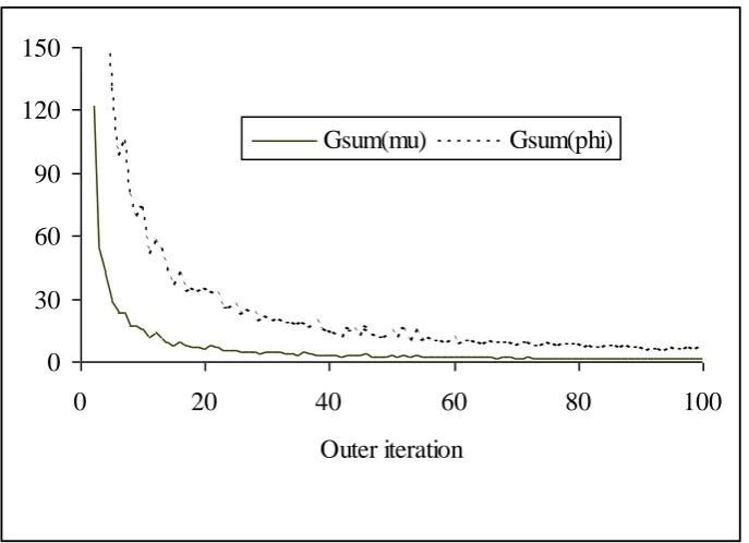
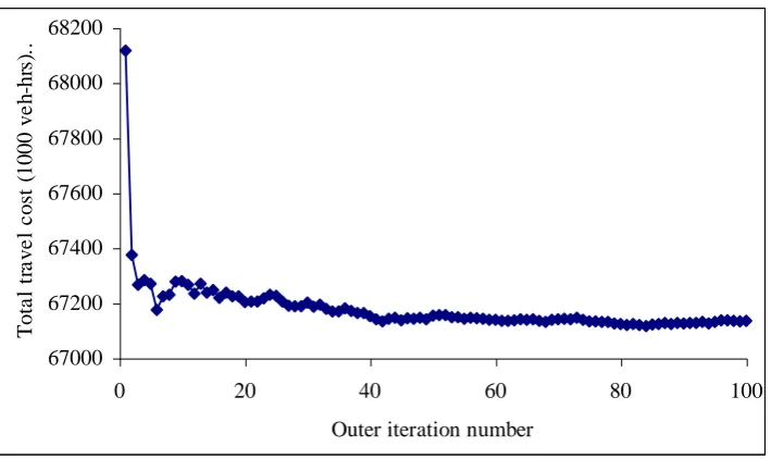
This same feature was observed for other choices of and , and for other output measures, as well as in the Sioux Falls case. A further investigation of the inner/outer iterations was therefore necessary. Figure 1
illustrates the flow similarity measures Gsum( )n ( ) and Gsum( )n ( ) given by (3.1), where is the vector of
GSUE(2) link flow variances, against outer iteration n. Figure 2 is the corresponding plot for total travel
cost. The figures indicate the characteristic stability of the GSUE(2) outer iterates observed in the tests
(including cases with lower values of nINNER), with convergence as measured by Gsum( )n (.) virtually
monotonic. The tests generally indicated that, in the two networks considered, the main effort was carried
out in the early outer iterationsin the cases considered, this means in the first 20-30 iterations. In contrast,
the inner iterations were in general seen to converge rather more slowly, with nINNER identified as the
primary cause of the differences observed across the columns of table 1. In particular, a single run of the
inner MSA algorithm for varying numbers of iterations nINNER was seen to produce a variation in output
measures of the same magnitude as that observed for varying (nOUTER,nINNER)together as in table 1.
Again, this convergence pattern was observed in both networks under a variety of parameter values.
The conclusion was that, for a given computational load, the estimated equilibrium values would be more
robust if the balance of effort favoured the inner, as opposed to the outer, iterations. The standard values
around 10 and 46 minutes respectively of run-time for the Sioux Falls and Weetwood networks, running on
a 120MHz PC under DOS). The possibility cannot be ruled out, of course, that these findings are specific to
the networks considered, and care should therefore be taken in uses of this algorithm on other networks, to
ensure that a similar robustness and convergence pattern prevails.
Sensitivity tests of the GSUE(2) model were then performed, with the particular aim of comparing the
mean GSUE(2) predictions with a conventional SUE. Firstly, varying the time period duration (results
not presented here) confirmed what was to be expected from the asymptotic result noted in section
2.1namely that as is increased, GSUE(2) mean flows/costs approach SUE values. It was decided to focus henceforth on the case 0.1, this low value chosen so as to emphasise any differences in the
models as distinct from potential convergence error.
The second sensitivity test considered the effect of varying the probit perceptual dispersion parameter .
As well as comparing SUE and GSUE(2), a modified form of SUE was also studied. The modified SUE has
mean link flows MOD exactly equal to SUE link flows, with a link flow covariance matrix MOD
subsequently computed from (2.4b) based on SUE route proportions pSUEi.e.
) ,
( SUE T
1
MOD
q p , with (,) given by (2.7). The modified SUE link costs are then
) ,
(MOD MOD
t
with t(,) given by (2.5). This modified SUE model effectively assumes the SUE route proportions to be the equilibrium route choice probabilities in the stochastic flow case, with the final cost
estimates of the modified GSUE(2) kind, but without any feedback to the choice process.
In fact, the modified SUE model is precisely what the GSUE(2) solution algorithm, specified in section 3,
yields after one outer iteration, since the algorithm is initialised at SUE flows. Therefore, in Figure 2, a
comparison can be made of the modified SUE model (the iteration 1 total travel cost) and the GSUE(2)
model (the converged solution). It is noticeable that the former is substantially higher than the latter, which
in turn is substantially higher than the unmodified SUE value of around 64800 (not shown). Moreover,
these differences are ‘real’ in the sense of being an order of magnitude greater than the differences obtained
by using different random number seeds (see Table 1).
Varying (0.050.5) in both networks confirmed this as a more general feature, namely that the total GSUE(2) travel cost was generally bounded below by the SUE value, and bounded above by the
modified SUE value. The former bound confirms the anticipated underestimation of expected costs that
Cascetta, 1989). The latter bound indicates that correcting for this underestimation in a post hoc manner,
without permitting drivers’ response to the modified expected costs, will tend to lead to an over-correction. This is because drivers will, where possible, re-route to avoid the most affected links, meaning that the
potential inflation in such a link’s cost is mitigated by a reduction in flow.
The results for the Weetwood network also showed a generally increasing disparity between the GSUE(2)
and SUE models with increasing , both in terms of total travel cost and mean link flows. The GSUE(2)
total travel cost rose from 1.8% greater than the SUE value at 0.05, to 3.5% greater at 0.5; the modified SUE model was a more constant 5%-6% greater than SUE. The maximum absolute difference
between the GSUE(2) and SUE models in any individual mean link flow rose from around 50
vehicles/hour at 0.05 to around 100 vehicles/hour at 0.5. The Sioux Falls network yielded
qualitatively similar results, although the difference between SUE and GSUE(2) total travel cost was rather
smaller. On an individual link level, an increasing disparity with an increase in was more clearly evident: the average absolute difference between GSUE(2) and SUE mean link flows rose from 4.0 at
05 . 0
to 13.2 at 0.5, with the difference in mean link costs rising from 6.7 to 26.3.
6. NUMERICAL EXPERIMENTS: COMPARISON OF GSUE(2) AND SP MODELS 6.1 Tests on the basic networks
The SP model was applied to the test networks described in section 5, using the simulation methods
described in section 4. In both networks, for both the SP1 and SP2 methods, and under a wide variety
of adjustments to the model parameters m,and (as well as factors applied to the demand matrix,
different random seed values, different initial conditions), it could be immediately observed that the
predictions produced were radically different to those arising from the SUE or GSUE(2) models. A
typical simulation is illustrated in Figure 3, based on a slight variant of the Weetwood network. A
quasi-periodic behaviour is evident, the period of the extreme points being almost exactly 10 (= m),
although the amplitude and period actually do vary due to the stochastic nature of the process. The extreme
points give rise to a total travel cost that is several orders of magnitude greater than that under a SUE or
GSUE(2) model. Figure 4 illustrates a corresponding behaviour observed for Sioux Falls.
In order to understand better such behaviour, consider the following simple example of an m-dependent
process, in which a single user has a choice between two routes, labelled ‘state 0’ and ‘state 1’. Let
deterministic, with S(0) transforming with probability 1 into state 1, and any other m-sequence
transforming with probability 1 into state 0. The unique, globally stable equilibrium behaviour is a
periodic motion of order m, with m days of state 0 followed by one day of state 1. It is possible to
establish this result by noting that an equilibrium probability distribution satisfying (2.11) is that which
puts equal probability mass 1 1
m at each of the sequences
S( ):j j 0 1 2, , ,...,m
; hence, from themarginal distributions of these equilibrium sequence probabilities, it follows that in equilibrium, state 0
occurs with probability mm1 and state 0 with probability 1 1
m . Now suppose instead that the transitions
truly are stochastic: S(0) transforming to states 0 or 1 with probabilities and 1, and S( j) )
,..., 2 , 1
(j m transforming to states 0 or 1 with probabilities1 and . For small and , Monte
Carlo simulations closely resemble the periodic behaviour of the deterministic system. A simple
network example of this behaviour is that with two parallel links with ~q1 d1, 1, m4,
9 ) (
1 v
t , 2
1
2( ) 10d v
t v , and 1( )
1 exp( ( 1 2))
1
u u
p u , for large values of 0.
The relevance of this example to model (2.12)/(2.13) may be explained as follows. Suppose that: (a)
many drivers choose to use a particular link on day n, and that (b) this causes the link to operate at a
flow level in a steep part of the link’s power-law cost-flow performance function. Then the experienced travel cost on day n will be very high, thus deterring drivers from using that link on subsequent days. If
the experience is sufficiently bad, then they will be deterred from using the link on days
m n n
n1, 2,..., , until at the start of day nm1, they forget the bad experience on day n (the Markov property). Now they will take account of the travel costs that prevailed on days
m n n
n1, 2,..., , and precisely because the link was perceived to be unattractive on those days, it
will have had a low use and hence a low actual travel cost on those days. This means that on day
1
m
n , this link will now be perceived as an attractive choice for many drivers, and the whole cycle
which began on day n is now repeated.
Clearly this analogy is based on the two suppositions (a) and (b). In the case studies considered here,
supposition (a) is effectively controlled by the probit perceptual dispersion parameter , and supposition
(b) by the nature of the cost-flow performance functions, and the learning parameter m. Even for large
values of and m, which weaken these suppositions, the test networks exhibited similar quasi-periodic
In particular, it is the nature of BPR cost functions that they may give unreasonably high costs at flows well
over capacity. Of course, this has a potential impact on conventional equilibrium models, yet in that case
the effect is only “transient”, in the sense that if such extreme costs occur during the course of some
solution algorithm, then the effect will be simply to deter drivers from using such a route in the final
equilibrium solution. In the SP case, on the other hand, these extreme cost levels may affect (and indeed be
the predominant factor in) the final, stationary behaviour of the process, as we have seen above. This is
highly undesirable, since such functions are not intended to give a good representation of over-capacity
behaviour, but have been conventionally defined over a wide range of flow levels purely for operational
reasons of equilibrium solution algorithms.
The numerical results show, then, that there are cases where the SP and SUE/GSUE(2) models are
radically different. In fact, in cases such as this the predominant element in the SP is the dynamics between
days, even in the stationary phase, such as between-day autocorrelations; the GSUE(2) model, on the other
hand, can at best hope to capture the moments of the marginal distribution of flows for any particular day.
The tests indicated a significant causal factor to be the over-capacity region of the cost-flow performance
functions, and so further attention should be paid to this factor (see section 6.2).
As an aside, it is also worth noting the potential pit-falls in model-users interpreting the results of the SP
model. In order to test different initialisations of the process, the mean perceived costs on the first m1
days was set to (i) a pure average of previously-experienced travel costs, or (ii) a weighted average of
experienced costs and SUE costs, by introducing mk identical “dummy” SUE travel cost experiences at
the start of day k. Although the same behaviour ultimately prevailed in both cases, method (ii) was seen on
occasion to delay the onset of the quasi-periodicity for a potentially very long period. In such simulations,
the initial transient behaviour was seen to be a long period of days with flows varying randomly about an
apparently stable mean, with the stationary quasi-periodicity only later becoming evident.
6.2Tests on the modified networks
In view of the potential impact of the cost-flow functions, noted in section 6.1, modified forms of the
cost-flow relationship is assumed to apply to under-capacity flows, with cost increasing linearly with flow
over capacity, according to deterministic queuing delay (Van Vuren & Van Vliet, 1992, p. 104).
The SUE, GSUE(2) and SP models were all re-run with these modified functions for both test networks
and both the SP1 and SP2 methods, again in a variety of scenarios. (A further minor modification was, for
all tests, to set to zero any demand rates q where k qk0.5, in order to minimise the effect of losing
trips when qk is “integerised” for the application of the SP model.) At lower values of m and/or , the
quasi-periodicity previously evident in the SP model was still apparent, but now with extreme points giving
total network travel times that were of a similar order of magnitude to the non-extreme days. As m was
increased, the quasi-periodicity gradually disappeared. However, one negative side to this modification was
that the SUE and GSUE(2) mean predictions were much closer than in the pure BPR case. This is to be
expected, since for any flows in the linear regime of the cost-flow functions, there will be no difference in
the standard and modified expected cost relationships (the second derivatives are zero). In the Sioux Falls
network, it was seen that under a variety of parameter values, the SP model’s predictions approached those
of the SUE/GSUE(2) model as m became large (up to m50). On the other hand, the similarity between the two equilibrium models meant that it was not possible to distinguish whether the GSUE(2) model was
closer than the SUE model to predicting the mean flows of the SP.
The Weetwood network presented more interesting results, a sample set given in Table 2 (the cases m =
100 and 200 were also tested, but gave identical results to m = 50 up to the accuracy in the table). The SP
results were obtained from a simulation of 1000 days, with the first 200 discarded in estimating stationary
moments. The results for the SP2 method (with nSAMP 30) are given in brackets, following the
unbracketed results which are from the SP1 method. The abbreviation ‘AAD’ refers to Average Absolute
Difference. The SP1 and SP2 results clearly follow a similar pattern, and so we may henceforth safely
restrict attention to one (SP1, say). For comparison, the SUE total travel cost was 245.9, and the GSUE(2)
one 246.1, so in terms of this global measure it is difficult to differentiate between the two models, relative
to the SP results for the case m50. However, at the level of individual link flows and link costs, then a
distinction is possible, with the AAD in mean flows and mean costs ultimately (for sufficiently large m)
smaller for the GSUE(2) vs SP comparison than for the SUE vs SP comparison.
m Total travel cost (105 veh-hrs) SP1 (SP2)
AAD in SUE vs SP mean flows
SP1 (SP2)
AAD in SUE vs SP mean costs
SP1 (SP2)
AAD in GSUE(2) vs SP mean flows
SP1 (SP2)
AAD in GSUE(2) vs SP mean costs
3 422.6 (426.3) 233.1 (253.8) 46.0 (45.3) 236.4 (255.9) 46.2 (45.6)
5 370.6 (332.0) 185.7 (137.5) 38.4 (27.9) 187.6 (138.1) 38.2 (27.9)
10 283.1 (281.8) 71.7 (67.3) 16.9 (16.3) 70.7 (68.2) 16.5 (16.0)
20 246.4 (247.6) 29.6 (31.1) 4.2 (4.7) 27.6 (29.3) 3.8 (4.3)
30 242.4 (241.9) 22.0 (20.9) 2.3 (2.0) 20.2 (18.4) 1.8 (1.4)
[image:23.595.41.544.70.197.2]50 240.7 (241.6) 18.6 (19.8) 1.7 (1.9) 14.9 (17.0) 1.2 (1.3)
Table 2: Comparison of SP, SUE and GSUE(2) models, for SP1/SP2 methods (Weetwood; 0.3;0.1;nSAMP 30;modified BPR functions)
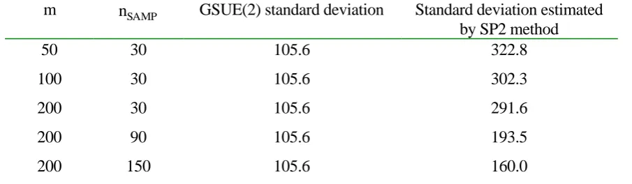
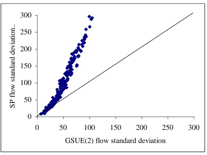
For the GSUE(2) and SP models, further comparisons are possible in terms of their predictions of link
flow variances. The results from the SP1 and SP2 methods are rather different here, and so they are
considered separately. From first comparisons with the SP2 method, a pattern was immediately clear,
namely that, on a link-by-link comparison, the equilibrium variances estimated by the SP2 method
were higher than their GSUE(2) counterparts, and that the absolute discrepancy was greater for links
with the higher flow variances. These patterns indicated a useful measure of discrepancy to be the
difference between the SP2 and GSUE(2) link flow standard deviation on the link with the highest
GSUE(2) flow standard deviation. The value of this measure under a variety of values of m and nSAMP
is given in Table 3. (The parameter nSAMP is defined in section 4). Furthermore, for two such cases a
link-by-link comparison of flow variances is given in Figures 5 and 6, neglecting links with a flow rate
standard deviation of less than 5 vehicles/hour.
m nSAMP GSUE(2) standard deviation Standard deviation estimated
by SP2 method
50 30 105.6 322.8
100 30 105.6 302.3
200 30 105.6 291.6
200 90 105.6 193.5
200 150 105.6 160.0
Table 3: Comparison of flow variance estimated by GSUE(2) and SP2 methods, for the link with highest variance (Weetwood; 0.3;0.1; modified BPR functions)
While the discrepancy between the two sets of figures is partially attributable to a “real” effect, namely that
the GSUE(2) model effectively assumes an infinite m, there is a substantial residual effect due to nSAMP. In
[image:23.595.66.519.496.628.2]As would be expected, this error leads to an overestimation of variance, due to the day-to-day varying error
in the estimated choice probabilities. The fact that the SP2 method can produce acceptable estimates of
mean flows (see Table 2 and surrounding discussion), while producing poor estimates of flow variances,
can indeed be observed in much simpler examples. For example, for a network with two parallel links,
constant cost functions t1(v)5, t2(v)7 , q1 200, 1 and 0.3, the constant probit choice probability for route 1 may be verified to be around 0.78, using tables of Normal probabilities. The SP
daily flows coincide with the binomial GSUE(2) moments in this special case of flow-independent costs,
yielding a route 1 flow rate mean and variance of 1 q10.78156 and
3 . 34 ) 78 . 0 1 ( 78 . 0
1 1
1
q respectively. Estimating these same measures by the SP2 method
yields Table 4, where values of nSAMP as large as 300 can produce poor variance estimates.
SAMP
n ˆ1 ˆ1
300 156.1 56.2
600 156.3 45.1
900 156.0 41.5
[image:24.595.127.465.692.765.2]1200 156.2 36.3
Table 4: Estimates of mean and variance in flow rate by SP2 simulation method (two link, constant cost network)
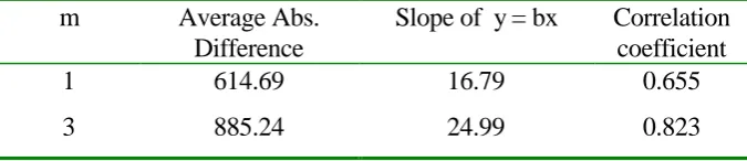
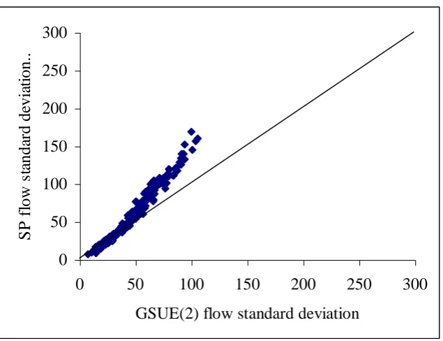
Focusing, then, on the SP1 method, Table 5 provides the results of a link-by link comparison of the
standard deviations estimated by SP1 and GSUE(2), again for links with a standard deviation of at least 5.
For each value of m, the figures reported are: the average absolute difference across links; the slope of a
least squares regression fit with zero intercept; and the correlation coefficient. The clear pattern is one of
increasing similarity between the two models as m is increased. As would be expected, the SP model gives
rise to generally greater variances at lower values of m, as can be seen from the ‘slope’ column. On the
other hand, at values of m as high as 30 there remains a substantial discrepancy between the variances
predicted by the models. The case m = 200 is further illustrated in Figure 7, where a close correspondence
across all links is evident. It is noted finally that comparisons were also made with the ‘modified SUE’
model, as defined in section 5. While the margin was not great, perhaps due to the linear regime of the
cost-flow curves, the evidence was of GSUE(2) being closer than modified SUE to the SP predictions.
m Average Abs.
Difference
Slope of y = bx Correlation coefficient
1 614.69 16.79 0.655
5 861.32 23.81 0.738
10 556.47 16.43 0.804
20 162.71 5.67 0.662
30 73.38 3.01 0.495
50 5.11 1.11 0.961
100 2.31 1.01 0.994
[image:25.595.126.469.71.219.2]200 1.89 0.98 0.996
Table 5: Comparison of link flow standard deviations estimated by GSUE(2) and SP1 methods (Weetwood; 0.3;0.1; modified BPR functions)
7. CONCLUSION
A solution algorithm has been presented for directly computing link flow means, variances and covariances
for the GSUE(2) model. The numerical experiments have confirmed that this method is efficient for large
realistic networks, as well as displaying desirable convergence and reproducibility properties. In contrast,
the estimation of the SP model by Monte Carlo simulation has a number of dangers for the model-user. In
particular, it has been seen how seemingly plausible model assumptions may induce autocorrelations,
evident in a quasi-periodic equilibrium behaviour of the simulation, which could not reasonably be viewed
as the plausible day-to-day operation of a network.
This paper has clearly not examined the full potential of the SP approach, with only a small part being
considered of the wide range of model assumptions that can be accommodated. However, the difficulties
noted are certainly not restricted to the relatively simple macroscopic models of the kind considered here,
with complex quasi-periodic behaviour having been observed in microscopic models of day-to-day route
choice and vehicle movement (Nagel & Barrett, 1997; Liu et al, 1999). It is intended that in this respect,
the GSUE(2) model may prove complementary to the SP approach (rather than a competitor), in helping to
understand the nature of SP solutions and to identify potential numerical estimation problems. In particular,
the numerical evidence gathered in this paper suggests that a useful preliminary step in an SP application is
to attempt an understanding of the differences between the SP model run with a large value of m and the
results from the GSUE(2) model. As discussed in Watling (2001), the GSUE(2) model should not itself be
regarded as a fixed entity, with many extensions possible (e.g. within-day dynamics).
The general approach of using approximation methods to gain an understanding of complex SP and