l
'-Y/ ').
AFIPS
CONFERENCE
PROCEEDINGS
VOLUME 23
1963
SPRING JOINT
COMPUTER
CONFERENCE
1963
SPARTAN BOOKS, INC. Baltimore, Md.
those of the authors and are not necessarily repre-sentative of or endorsed by the 1963 Spring Joint Computer Conference Committee or the American Federation of Information Processing Societies.
Library of Congress Catalog Card Number: 55-44701
Copyright © 1963 by American Federation of Information Processing Societies, P. O. Box 1196, Santa Monica, California. Printed in the United States of America. All rights reserved. This book or parts thereof, may not be reproduced in any form without permission of the publishers.
Sole Distributors in Great Britain, the British Commonwealth and the Continent of Europe:
CLEA VER-HUME PRESS
10-15 St. Martins Street London W. C. 2
1. 1951 Joint AlEE-IRE Computer Confer-ence, Philadelphia, December 1951 2. 1952 Joint AIEE-IRE-ACM Computer
Conference, N ew York, December 1952 3. 1953 Western Computer Conference, Los
Angeles, February 1953
4. 1953 Eastern Joint Computer Conference, Washington, December 1953
5. 1954 Western Computer Conference, Los Angeles, February 1954
6. 1954 Eastern Joint Computer Conference, Philadelphia, December 1954
7. 1955 Western Joint Computer Conference, Los Angeles, March 1955
8. 1955 Eastern Joint Computer Conference, Boston, November 1955
9. 1956 Western Joint Computer Conference, San Francisco, February 1956
10. 1956 Eastern Joint Computer Conference, New York, December 1956
11. 1957 Western Joint Computer Conference, Los Angeles, February 1957
12. 1957 Eastern Joint Computer Conference, Washington, December 1957
13. 1958 Western Joint Computer Conference, Los Angeles, May 1958
14. 1958 Eastern Joint Computer Conference, Philadelphia, December 1958
15. 1959 Western Joint Computer Conference, San Francisco, March 1959
16. 1959 Eastern Joint Computer Conference, Boston, December 1959
17. 1960 Western Joint Computer Conference, San Francisco, May 1960
18. 1960 Eastern Joint Computer Conference, New York, December 1960
19. 19til Western Joint Computer Conference, Los Angeles, May 1961
20. 1961 Eastern Joint Computer Conference, Washington, December 1961
21. 1962 Spring Joint Computer Conference, San Francisco, May 1962
22. 1962 Fall Joint Computer Conference, Phil-adelphia, December 1962
23. 1963 Spring Joint Computer Conference, Detroit, May, 1963
Conferences 1 to 19 were sponsored by the National Joint Computer Com-mittee, predecessor of AFIPS. Back copies of the proceedings of these con-ferences may be obtained, if available, from:
• Association for Computing Machinery, 14 E. 69th St., New York 21, N. Y. • American Institute of Electrical Engineers, 345 E. 47th St.,
New York 17, N. Y.
• Institute of Radio Engineers, 1 E. 79th St., New York 21, N. Y.
Conferences 20 and up are sponsored by AFIPS. Copies of AFIPS Con-ference Proceedings may be ordered from the publishers as available at the prices indicated below. Members of societies affiliated with AFIPS may obtain copies at the special "Member Price" shown.
Volume List Member Publisher
Price Price
20
21
22
23
$12.00 $7.00 Macmillan Co., 60 Fifth Ave., New York 11, N. Y.
6.00 6.00 National Press, 850 Hansen Way, Palo Alto, Calif.
8.00 4.00 Spartan Books, Inc., 301 N. Charles St., Balti-more 1, Md.
10.00 5.00 Spartan Books, Inc., 301 N. Charles St., Balti-more 1, Md.
NOTICE TO LIBRARIANS
This volume (23) continues the Joint Computer Conference Proceedings (LC55-44701) as indicated in the above table. It
is suggested that the series be filed under AFIPS and cross referenced as necessary to the Eastern, Western, Spring, and Fall Joint Computer Conferences.
Page
vii Preface
1
9
17
29
41
51
59
ALGORITHMS IN BUSINESS DATA PROCESSING Determining Fastest Routes Using Fixed Schedules
Equitable Distribution
RAMPS-A Technique for Resource Allocation and Multi-Project Scheduling
MACHINE ORGANIZATION I Time Sharing on the Ferranti-Packard
FP6000 Computer System
The D825 Automatic Operating and Scheduling Program
A Time-Sharing Debugging System for a Small Computer
Experience with the Atlas Scheduling System
ANALOG AND HYBRID SYSTEMS I
69 DYSAC: A Digitally Simulated Analog Computer
83 DAS: A Digital Analog Simulator
91 Six Degree-of-Freedom Simulation of a Manned Orbital Docking System
105 Application of Hybrid Analog and Digital Techniques in the Automatic Map Compilation System
DATA ACQUISITION TRANS 1M ISS ION AND DISPLAY
113 Automatic Reading :Machine for Telegraph Service 117 A Research Laboratory for Processing and Displaying
Satellite Data in Real Time
127 A Real Time Multi-Computer System for Lunar and Planetary Space Flight Data Processing
141 Ground Operation Equipment for the Orbiting Astronomical Observatory
155 Error Detection Correction and Control
B. M. LEVIN S. HEDETNIEMI J. A. GOSDEN J. MOSHMAN J. JOHNSON M. LARSEN
F. M. MARCOTTY F. M. LONGSTAFF
A. P. M. WILLIAMS
R. N. THOMPSON J. A. WILKINSON S. BOlLEN
E. FREDKIN J. C. R. LICKLIDER J. MCCARTHry D. J. HOWARTH
J. R. HURLEY
J.
J. SKILES R. A. GASKILL J. W. HARRIS A. L. McKNIGHTJ. C. Fox T. G. WINDEKNECHT S. BERTRAM
W. D. BUCKINGHAM R. H. SPITLER B. K. KERSEY W. HOOVER A. ARCAND T. B. MILLER A. G. FERRIS
E. J. HABIB H. W. COOPER R. L. MCCONAUGHY R. STEENECK
Page vii
1
9
17
29
41
51
59
69
83
91
105
113 117
127
141
CRITICAL ANALYSES OF THE CURRENT STATE OF THE ART
163 State of the Art in Scientific Computing R. W. HAMMING 163
169 State of the Art of Programming R. S. BARTON 169
179 Computer Applications for Industry and the Military: D. F. BLUMBERG 179 A Critical Review of the Last Ten Years
ANALOG AND HYBRID SYSTEMS II
191 Automatic Parameter Optimization as Applied to M. HOWELL 191
Transducer Design
197 Hybrid Computer Solution of Time-Optimal Control E. G. GILBERT 197
Problems
205 Multiple Integrals on a Non-Repetitive Analog Computer A. HAUSNER 205
213 Hybrid Techniques for Analog Function Generation W. E. CHAPELLE 213
INFORMATION RETRIEVAL
229 Automatic Stratification of Information D. LEFKOVITZ 229
N. S. PRYWES
241 A Computer Approaeh to Content Analysis: Studies P. J. STONE 241
U sing the General Inquirer System E. B. HUNT
257 Selective Dissemination of Information (SDI) : State of C. B. HENSLEY 257 the Art in May, 1963
263 Computer Controlled Printing M. P. BARNETT 263
D. J. Moss D. A. LUCE K. L. KELLY
289 On the Solution of an Information Retrieval Problem B. H. SAMS 289
COMPUTER AIDED DESIGN
299 An Outline of the Requirements for a Computer-Aided S. A. COONS 299
Design System
305 Theoretical Foundations for the Computer-Aided Design D. T. Ross 305
System J. E. RODRIGUEZ
323 Man-Machine Console Facilities for Computer-Aided R. STOTZ 323
Design
329 Sketchpad: A Man-Machine Graphical Communication 1. E. SUTHERLAND 329 System
347 Sketchpad III: A Computer Program for Drawing in T. E. JOHNSON 347
Three Dimensions
MACHINE ORGANIZATION II
355 Key Addressing of Random Access Memories by A. D. LIN 355
Radix Transformation
367 ADAM-A Problem-Oriented Symbol Processor A. P. MULLERY 367
R. F. SCHAUER R. RICE
381 Associative Techniques with Complementing Flip-Flops E. S. LEE 381
395 Physical and Logical Design of a Highly Parallel Computer J. S. SQUIRE 395 S. M. PALAIS
MANNED SPACECRAFT SIMULATION
401 Introduction to the Panel Discussion J. H. McLEOD 401
410 Reviewers, Panelists, Session Chairmen and Panel 410
Moderators
411 1963 Spring Joint Computer Conference Committee 411
412 AFIPS Committees 412
414 Exhibitors 414
This volume contains the full text of the thirty-seven technical papers selected for presentation and discussion at the 1963 Spring Joint Com-puter Conference. It also includes a summary of one of the special panel discussions. Thus it provides a permanent record of the more formal side of the Conference.
The material herein represents a broad cross-section of activity in computer and information-processing technology, as of early 1963. In organizing the program for the Conference, general areas of interest were tentatively established for each session, and these were used as guides in selecting and grouping papers. On the whole, however, no real constraints were imposed as to subject matter.
Indicative of the scope are three papers devoted specifically to critical analyses of the current state-of-the-art. In other papers, the subjects dis-cussed range from basic concepts to practical applications, in both hard-ware and softhard-ware, reflecting the ever-broadening impact of information processing on modern society.
This volume is the product of much hard work on the part of the authors who prepared the individual papers. We are indeed grateful for these contributions-clearly the backbone of any highly technical Con-ference such as this. It is also a pleasure to acknowledge the contributions of the many others-well over a hundred-who helped organize the Con-ference and who participated as session chairmen, panel moderators, panelists, and reviewers.
E. CALVIN JOHNSON General Chainnan
Dr. Bernard M. Levin and Mr. Stephen Hedetniemi National Bureau of Standards
Washington 25, D.
c.
INTRODUCTION
An interesting problem that is amenable to solution by digital computer is posed by the following questions. How late can a shipment be detained at city A so that it arrives at city B by a given time? By what route should it be sent? The available routes consist of those provided by scheduled common carriers such as the airlines.
In some situations, no single scheduled carrier trip satisfactorily connects the two cities involved. In such a case it might be necessary to rise two vehicles and to transfer the mail between the two at a third city. Con-ceivably, it might be necessary to use three or more vehicles and two or more transfer points. The problem may have more meaning if it is posed by the following more personal questions. How late can I stay in my home town and still get to an appointment in another city on time? What route should I take?
An important application of a solution to this problem can be found in the Post Office Depart-ment. The Department tI'ies to pyocess :mail received in the afternoon so that it will be delivered the following morning at distant cities.
This problem has been studied at the National Bureau of Standards under the sponsorship of the Post Office Department. This paper de-scribes and discusses some solutions that have been obtained. These solutions are related to and stem from published literature regarding the Shortest Route Problem.
1
THE PROBLEM
Relationship to the Shortest Route Problem Given a network of points and lines, the latter numbered by the distance between the points they connect, it may be of interest to know the shortest path between any two points. This is the shortest route problem and many solutions to this problem appear in the litera-ture.I, 3, 5, 7
is not the shortest route, but it may be the desired one.
Factors to be Considered
If our only consideration is to leave Boston as late as possible in order to make our luncheon appointment, then the routing by way of Idle-wild is superior because it leaves 75 minutes later than the direct flight. There are, however, other factors that must be taken into considera-tion in deciding which routing is superior, in addition to flight time and departure time.
1. Cost: It costs $21.80 to fly directly from Boston to Binghamton. It costs $28.80 to fly from Boston to Idlewild to Binghamton. In other words, we must pay seven dollars plus tax for the extra 75 minutes of sleep.
2. Reliability: The routing by way of Idle-wild allows 52 minutes for transferring from the Boston-Idlewild plane to the Idlewild-Bing-hamton plane. If the Boston-Idlewild plane were late, the connection might be missed, caus-ing us to be stranded at Idlewild and, therefore, to miss our luncheon. And further, if the Idle-wild-Binghamton plane were late, we mig}1t also miss our luncheon. Also~ any scheduled air-line flight is subject to cancellation due to weather or equipment problems. The direct flight from Boston to Binghamton involves only one plane and therefore such problems are less likely to occur than in the two plane routing by way of Idlewild. In other words, to get 75 minutes more sleep, we would increase the probability of not arriving by the required time. 3. Transfer time: We have considered the problem of missing connections due to the late arrival of the first plane in a two-plane routing. Even if the first plane is on time, some time must be allowed for transferring from it to another plane. This time varies according to the size of the airport and according to whether or not the transfer is between two planes of the same airline or between planes of two different airlines. The recommended minimum time for transferring at Idlewild from the Boston-Idle-wild flight to the IdleBoston-Idle-wild-Binghamton flight is 30 minutes, which is less than the available 52 minutes. In addition to the 7 :45 a.m. flight, there is a plane from Boston to Idlewild leaving Boston at 8 :30 a.m. arriving at Idlewild at 9 :22 a.m., only 8 minutes before the departure from Idlewild to Binghamton. We would not select
this flight because eight minutes is not sufficient transfer time.
In summary, we have stated five factors that are of importance in selecting routes: (1) de-parture time, (2) cost, (3) reliability, (4) transfer time, and (5) arrival time. The only required property of the arri~al time is that it be before a specified time.
PRELIMINARY SOLUTIONS
Selection of Flights Along a Known Route A digital computer can be programmed to select flights along a known path. For example, the known path could be Boston to Idlewild to Binghamton. There are several flights each day between both pairs of airports. The computer can be programmed to select the set of flights that best meets the criteria discussed in the previous section. Only the criterion of time will be discussed in this section.
To simplify matters, the procedures in this paper will be described by means of terminology peculiar to airline flights. The procedures can be used for air transportation, surface trans-portation, and for combinations of surface-air transportation.
The selection of the flights is not as simple a task as it may at first appear. One solution would be to check all possible combinations of flights. While this is simple conceptually, it involves an inefficient use of the computer. Another obvious approach would be to select a desirable departure time from Boston and choose the flight to Idlewild with the departure time closest to this desired time. The first flight leaving. Idlewild for Binghamton after the arrival of the selected Boston-to-Idlewild flight would be the selected second link flight. This solution is efficient but has two important short-comings which are easy to overcome:
1. It overlooks some problems involved in making transfers.
2. It is not designed to answer one of the specific questions asked, namely, that of leaving as late as possible.
called an inter-line transfer. The minimum time allowed to make a transfer is usually less in the first case than in the latter. There is no problem in having two minimum transfer times for each airport: one for intra-line transfers and one for inter-line transfers. The problem arises when the first flight to arrive requires an inter-line transfer and a second flight, which arrives soon afterward, involves an intra-line transfer. It is possible that the earlier flight cannot make connections with the plane which departs at the desired time, while the later flight can. For example, suppose there is a flight from city A to city B leaving at 7 :00 and arriving at 8 :00 on airline one. Suppose there is also a flight between the same two cities leav-ing at 7 :05 and arrivleav-ing at 8 :05 on airline two, and there is a flight on airline two departing city B for city C at 8 :45. If intra-line transfers require 30 minutes and inter-line transfers re-quire 60 minutes, then the flight which arrives at 8 :05 can make connections, while the 8 :00 flight cannot. The solution to this problem of transfer times is to consider as potential first-link flights all flights whose arrival. time at city B is within X minutes after the earliest arrival time at city B, where X is the difference between the inter-line and intra-line transfer times at city B. In cases of routes having more than one transfer point, this factor must be considered at each transfer point.
The problem posed in Section I was to select a routing that permitted the shipment to be detained at the originating city as late as possible. The solution described so far uses a prescribed earliest departure time and, therefore, does not really solve the problem posed. This can easily be corrected by tracing the route backwards. The last leg of the trip would be selected first, based on its arrival and departure times, and so forth. The basic nature of the solution would be unchanged. In over-cOiuing the transier problem described in the previous paragraph, we would consider as potential last link flights all flights whose de-parture time at city B is within X minutes be-fore the latest departure time at city B.
Selection of Promising Routes
The backward tracing of the path with proper correction for the transfer problem will select the optimum path on a basis of the
cri-terion of latest departure. However, it requires the routing to be predetermined. In order to find the best set of flights, it will often be necessary to trace out numerous routes. These routes can be determined by another com-puter program or by someone making decisions regarding the routes to be tested. An algorithm has been developed which finds the N short-est routes between two given cities where
Nl
<
N <N'2' and Nl and N2 are variables. Thisalgorithm considers only the travel time among the cities and does not consider delays involved in transferring. It will be the subject of a separate paper now being prepared. (It would ha ve been possible also to have used other pro-cedures for finding the N shortest routes.) 2, 4
For each of the N routes, a set of flights is selected and compared with the sets of flights for the other routes, and the set of flights with the latest departure time selected. A computer program has been written which selects the N
shortest routes neglecting transfer times, se-lects a set of flights for each route considering transfer times, and rank orders them on the basis of latest departure time. This program uses as input data IBM cards containing the name of the airline, the flight number, the de-parture airport and time, and the arrival airport and time. It can handle 2,000 trip segments and 45 transfer points. To save space in the computer memory, a trip that has several stops is considered as a series of nonstop trip seg-ments. For example, a plane trip from Boston to N ew York to Washington is treated as two trip segments: Boston to New York and New York to Washington.
The program was written in FORTRAN for the IBM 704 and 7090 computers. On the IBM 7090, it took two minutes to find paths between 30 pairs of cities. This involved determining and tracing 265 paths.
There is no assurance that the best route will be one of the N shortest routes as determined by the algorithm. All of the N shortest routes may involve poor connections at the transfer points while a longer routing may involve good connections at the transfer points. This is a weakness of the procedures. Also, cost is not considered.
departure time at the city of origin is deter-mined, consideration can be given to selecting the earliest arrival time. The airline passenger may wish to depart as late as possible, but he would prefer having idle time in the city of destination rather than at a transfer point. In the same way, we may want to have the depar-ture of the last dispatch of mail as late as pos-sible. (Mail ready for an early dispatch would be sent on the early one.) However, once the dispatch time is set, it would be desirable to get the mail to its destination as early as possible so that there would be more time to process it at the destination post office. This can be ac-complished by retracing the path in a forward direction after the departure time has been de-termined by the backward tracing. For ex-ample, if we wish to leave Minneapolis and arrive at Cleveland by 7 :00 p.m., we would find, by tracing backwards, that we could take a 3 :45 plane from Chicago, arriving in Cleveland at 6 :20. We could take a 1 :45 plane from Minneapolis to Chicago and connect with the 3 :45 plane. Tracing forward, we find we could take the 1 :45 plane from Minneapolis and make connections in Chicago with a plane arriving at Cleveland at 6 :05, fifteen minutes earlier than the trip selected by the backward tracing.
Selection of Optinl,um Routes
A computer program has been written that does not have the limitations just described. It
always finds the fastest route; it includes cost as a factor; and it does not require both a for-ward and backfor-ward tracing. It is based on the algorithm presented in the Appendix (with modifications indicated below) and is sinlilar to a procedure suggested by Minty5. The basic idea is to find the best direct flights given a starting time from the originating airport to all other airports being considered. The direct flights are the links of the network. Each of these selected direct flights is considered as a possible first link of a two-link route to each of the other airports. The airport at which the direct flight lands is considered as a potential transfer point. Every flight leaving that airport is paired with the direct flight, Ea.ch resulting two-link route is compared with the best previ-ously determined route to the arrival city of the two-link route. If it is better, it is stored in place of the previously determined best. After all the stored one-link routes are tested, the
stored two-link routes are tested to see if they can be used as the first two links of a usable three-link route. Whenever the three-link route is better than the previously stored route, it is stored in place of the previous best. This proc-ess is continued until for some m, all of the m-link stored routes are tested as the first m links of a route having m+ 1 links, and none of the (m+ 1) -link routes warrant retention. This algorithm is similar to the "Moore Algorithm"4. . The transfer problem described in the previ-ous section arises here also. I t is solved by storing more than one route between a pair of cities whenever conditions warrant, and using each of the stored routes to see if it can be the first part of a route to another city. The criteria for storing additional routes are the same a..~
before. That is, consider as potential first-link flights all sets of flights along any route whose arrival time at city B is within X minutes after the earliest arrival time found so far at city B,
where X is the difference between inter-line and intra-line transfer times at city B.
It should be noted that this solution finds routes not only from the origin city to the des-tination city but also from the origin city to all other cities. Hence, some routes are retained only because they are promising routes to po-tential transfer points; other routes are re-tained because they are tentatively the best routes to a city as well as because they are promising routes to potential transfer points. As described above, the solution is geared to an originating time rather than to a desired arrival time. Another approach would have the
program "1yvork from a desired arrival time and find the latest possible departure time from each of the other cities to that city. After the departure times are found, the earliest arrival times to the destination city based on each of the computed departure times could be deter-mined. However, the approach described below should be more desirable because it finds good routes (fastest for some departure time) for all times of day in an efficient manner. If good routes for all times of day are known, the de-sired route for a given arrival time can easily be selected. The best routes for all times of day can be computed by means of the approach that follows.
best routes for a new departure time, say 10 :30 p.m., could be cop.sidered in the following man-ner: Using as first links only flights which de-part between 10 :30 and 11 :30, new potentially useful multiple-link routes would be computed. In deciding whether or not to save a computed route, it must be compared with the best route found so far, which includes those routes based on the 11 :30 departure time. The computa-tions involved would be less time-consuming for this second departure time because a set of flights would be saved only if it is better than the retained 11 :30 departure routes. A third time, say 9 :30, could be selected and the process continued by selection of earlier times through-out the day. The final results will be the fastest routes from the origin city to all other cities for each departure time used. (Duplicate routes can be suppressed.) From this mass of data, the routing that best answers the question origi-nally posed can be selected. In addition, data are available to answer many similar questions. This solution involves one minor problem. This can best be described by an example. Sup-pose we wish to arrive at a given city by mid-night. If there are two direct flights, one which leaves at 10 :50 p.m. and the other at 10 :40 p.m. and both take an hour, the algorithm as de-scribed above would pick the flight with the earlier departure and arrival times, the flight leaving at 10 :40. The 10 :50 flight leaves later and would be the better flight according to the criteria described earlier in this paper. How-ever, the selected flight is so similar to the best flight that this cannot be considered an impor-tant problem, especially since the interval be-tween the departure times considered is subject to control.
An advantage of this approach is that a large amount of useful data is obtained in a system-atic fashion.
LATEST SOLUTION
Routes to Be Stored
There is one property of the algorithm in the Appendix that warrants emphasis. This property can best be described using the net-work in figure one. Assume node A is the origin point. The shortest routes to node B and node C are the direct links of four and three units length, respectively. We then try to develop
two-link routes to C, D, E, and F, using the link AB as the first link. The two-link route
ABC is nine units in length, which is longer than the direct link. Although we compute the link ABC, we do not retain it. The links ABD
and ABE, on the other hand, are retained. We then try using as a first link AC. The route
ACB is computed but rejected. The route ACE
(length 6) is computed and retained in place of the route ABE (length 8). In going through these operations we systematically consider all possible ways of extending each M link route to M
+
1 link routes. In developing three-link routes, the route ABD is extended to make the route ABDF and the route ACE is extended to make the route ACEF, which is longer than the stored route ABDF and is therefore ignored. The route ABDF is extended to the routeABDFE which is longer than the route ACE,
and therefore is not retained. In finding the route ABDF, the rule of using an M link route to fin d an M
+
1 link route still held. There was no need to use any other procedure to find this route, such as extending the route AB by two links at one time.Listing Procedure
In adapting the algorithm to find optimum transfer airports and flights, it is sometimes necessary to retain several routings from the origin airport to a given transfer airport. If time is the only criterion for the selection of an optimum route, the only criterion for re-taining non-optimum routes to potential trans-fer points is also time, where the amount of time is a function of the required minimum transfer times at that city. We need consider only the arrival times at that one point along the route; we need not worry about transfer problems at previous cities along the route nor at cities yet to be added to the route.
Additional Criteria
The introduction of the list procedure per-mits additional route-selection criteria to be introduced. In introducing additional criteria, it is necessary to be very specific. Additional criteria that have been introduced and pro-grammed are those of specific interest to the Post Office Department in routing air mail.
The Post Office Department pays for air transportation according to the following rules. 1. If only one airline is involved, the Post Office pays a loading charge based on the size of the airport plus a transportation cost based on the "short line distance" between the origin and destination airport. The short line dis-tances are the shortest disdis-tances between the two airports involved, using a single carrier. For example, suppose we wish to get from air-port A in Figure 1 to airport E and the routing we wish to consider is from A to B to E on air-line 1. If airair-line 2 has planes between airpor,t
A and C and also has planes between C and E,
airline one will be paid for only one loading charge and only six units of distance (the dis-tance of the ACE route) rather than the eight units of distance that the mail was transported.
A~ _______ 4 ________ ~~B
3
F
c
3~
E
2. If more than one airline is involved, the short line distance is paid each airline for any continuous portion of the route handled by that airline. An additional loading cost is added each time the mail is transferred from one air-line to another, based on the size of the airport at which the transfer is made.
It should be noted that when these rules apply, a straightforward application of the algorithm cannot answer questions regarding cost. However, as actual sets of flights are selected, costs can be computed. Whenever the fastest route is not the cheapest, the cheapest
route found can also be saved. Hence, the cri-terion of cost, as well as that of speed, can be taken into account.
The introduction of the criterion of cost with the costing rules described above creates some problems. If we consider the problem of getting from A to B by way of T, the following could happen. Let us say that the best flight from
A to T is on airline one, while airline two provides a flight which arrives much later. However, airline two provides the only service between T and B; therefore, the more time-consuming connections from A to T and B on airline two are cheaper, because there is no inter-line transfer cost. In other words, many poor flights and sets of flights must be retained and tested if it is required that the cheapest routing be found. This would greatly increase the computer time necessary. In order to make solutions practical, we have programmed the computer to select the cheapest set of flights that arrives at a transfer point less than X minutes after the fastest, where X is a variable set equal to, say, 120 minutes. Each of these selected sets is tested as the firstm links of a route having tn+ 1 links.
The problem of finding alternate routes when the fastest route does not operate every day is straightforward. Each computed routing can be tested to see if it is the fastest for any day of the week and if it is the fastest, it is -retained.
T he Pro gra,n
A computer program has been written and debugged using the techniques described in this section which does the following:
1. It finds the fastest route from an origin city or airport to all other cities or air-ports.
2. It finds "cheapest" routes, using the rules described above.
3. It finds alternate routes when the fastest route does not operate every day. 4. It finds routes for all times of the day,
using the procedure of finding the best flights for each of 24 different desirable departure times throughout the day, as described in section 3.
The program was written in FORTRAN, with F AP function subprograms used to pack and unpack data for the IBM 7090. It takes about one second to compute the "best" routes from one airport to the other nine airports in a ten airport network with 200 trip segments for a specified earliest departure time. This computation time does not include "set-up" time nor the time required to enter the data.
APPLICATIONS
The procedures described in this paper have many potential areas of application. Two such applications related to the Post Office problems will suffice as examples.
The Post Office Department prepares lists of multiple-link routes for the routing of air-mail. It is anticipated that the procedures de-scribed in this paper will be used instead of a hand operation to develop these routes.
The Post Office Department schedules many mail trucks to supplement service provided by common carriers. The techniques described in this paper can be used to evaluate a proposed revision of schedules.
There are, of course, many other areas of potential use. In most of these cases, a corre-sponding hand operation is now being used. It
is anticipated that computer procedures will be more efficient and more economical in many situations.
APPENDIX
A Computational Algorithm for Obtaining the Shortest Path From One Point to Every Other Point in a Network
Given a network of points Ph P:!, ... , Pm and lines between them, construct a distance matrix
A, with elements aij representing the length of
the line between points Pi and Pj' If no line exists between the points, let aij
=
00.The algorithm also applies to the situation where the lines are directional. The value of au would be the length of the line going from
Pi to Pj' It would not be necessary that aij
=
aji~Let ei contain the ordered sequence of points of the shortest path found so far from PI to Pi.
Let bi be the length of the shortest path found
so far from 1 to i. The original values will be the direct distances, i.e., the first row of matrix
A.
Let di indicate if the path ei has been used
in an attempt to create improved paths to other points. If di
=
0, it means it has been used,otherwise di = 1.
Let
f
= 1 if any di has been set equal to 1 sincethe last test of
f,
otherwise letf
=
o.
Steps (1) Set
Set Set (2) Set Set
(3) If
(4) Set
(5) If
(6) If
bi = ali
di = 1
ei = 1, i;
i = 2
f
= 0i = 2,3, ... , m
i = 2,3,' ... , m
i = 2,3, ... , m
di = 1, go to step 7
di = 0, go to step 4
i = i
+
11, ~ m, go to step 3 1,
>
m, go to step 6f
= 0, algorithm is finishedf
= 1, go to step 2(7) Set j = 2
(8) Compute c = bi
+
aij(9) If c ~ bj, go to step 11
(10)
(11) (12)
Set Set Set Set Set
If
(13) Set
c
<
bj, go to step 10 dj = 1ej = ei, J bj = c
f
= 1j = j
+
1j ~ m, go to step 8 j
>
m, go to step 13 di = 0Go to step 4
When the algorithm is finished, the contents of ei, i
=
2, 3, ... , m, will be the points through which a shortest path (more than one may exist) from PI to Pi passes. The values of bi , i = 2, 3, ... , m, will be the length of the shortest paths.It should be noted that the values of aij are
used only in step 8. At that time, trial value of bi is known and aij can be a function of that
value of bi • If bi is the time required to get to i and aij is the time from the arrival at i to the
arrival at j~ then aij can be determined from
published schedules using bi in determining the
earliest possible departure time at i.
REFERENCES
1. BELLMAN, RICHARD, "On a Routing Prob-lem." Quarterly of Applied Mathematics, vol. 16, p. 87-90. 1958.
2. BOCK, F., KANTNER, H., and HAYNES, J.,
Through a Network. Chicago, Armour Re-search Foundation of Illinois Institute of Technology, Technical Paper Number 19. 1957,
3. DANTZIG, G. B., "On the Shortest Route Through a Network." Management Science, vol. 6, p. 187-190. 1960.
4. HOFFMAN, \V., and PAVLEY, R., "A ~1ethod
for the Solution of the Nth Best Path Prob-lem." Journal of the Association for Com-puting Machinery, vol. 6, p. 506-514. 1959. 5. MINTY, GEORGE J., "A Variant on the
Shortest-Route Problem." Operations Re-search, vol. 6, p. 882-883. 1958.
6. 0 fficial Airline Guide, Quick Reference Edi-tion, vol. 6, No. 21. Chicago, Reuben H. Donnelley. 1962.
7. POLLACK, M., and WIEKENSON, W., "Solu-tions of the Shortest-Route Problem-A Review." Operations Research, vol. 8, p. 224-240. 1960.
John A. Gosden AUERBACH Corporation
1634 Arch Street Philadelphia 3, Pa.
THE PROBLEM OF DISTRIBUTION
The problem of distributing available re-sources occurs in a great variety of networks, each with peculiarities of its own. Coal from mines has to be distributed to central dumps and to small yards. Ice cream must be dis-tributed only to refrigerated stores and has a limited useful life. A buyer for a chain of stores with their own stock rooms but no central ware-house must indicate where his purchases are to be delivered. A farmer must distribute his labor according to the state of the crops and the weather, and many other distribution prob-lems exist in modern complex commercial life.
The problem of distribution is that the sum of the requests or needs of consumers does not equal the available supply. This is due in part to failures to meet production or buying plans, changes in consumer demand and other uncon-trolled variables, but also may be deliberate policy to maintain level production rates, to buy while raw material prices are favorable or to build up stock in expectation of peak demand periods such as Christmas or the Summer. The standard solution to the mis-matching of sup-ply and demand is the creation of buffer stocks.
In practice, there may be one or many buffer stocks in a network. In retail selling, there may be 5 levels-display stock, counter stock, shop stock, area depot stock and factory warehouse stocks-apart from stocks in the pipelines be-tween them. For all these, it is possible to establish optimum restocking periods and
opti-9
mum restocking levels. In ideal conditions, the total available for distribution would equal the sum of the amounts by which each store was under-stocked and allocations would be made to bring each to its optimum level at each re-stocking period.
To illustrate the principle of equitable dis-tribution, this paper considers an example con-sisting of a network in which there is one pro-duction site and several retail outlets. The whole network operates on a weekly cycle and the production in anyone week is available at the end of the week to replenish the retail out-lets. Each outlet has its own stock room but the production site carries no stock from week to week. Each week the forecasters estimate the weekly sales for each of the outlets. For example, suppose that it has already been estab-lished that at the beginning of each week the optimum restocking level of each of the outlets is ten days' estimated sales. The production plan, therefore, for anyone week consists of
.... hn "'.,~ ",4! .... hn ,.."' .... ~"""'n .... ,..rl "' ... 1,..", n~ ,.. ... ",1-, "' ... 1.,,+
I.I~H" "'U~U. V.1. IJU~ ~"'IJ~U.U;\.IJ~U QQ.l~Q V.1. ~Q\".ll VUIJ.lvlJ
plus any under-stock and minus any over-stocks held in the outlets at the beginning of the week. If all goes well, production meets its targets, the sales volume is exactly that estimated and then the production is exactly sufficient to re-stock the outlets to their optimum levels at the end of the week.
effects. First, production may be above or below that planned. Second, the actual sales may differ from those estimated. Third, the optimum restocking quantities may alter be-cause estimates of future sales are revised. In such a situation, either the requirements of the outlets exceed the production volume and some form of under-supply must be imposed or pro-duction volume is in excess of the requirements of the outlets and some form of over-supply must be imposed.
There are two important restrictions which must also be taken into consideration. The first restriction is that no allocation shall be made that causes the stock level in an outlet to exceed the capacity of its stock room. The second restriction (which does not occur in all situa-tions) is that no returns of stock from outlets or transfers among outlets are allowed. This latter restriction is a frequent feature of dis-tribution networks.
Numerical Example I
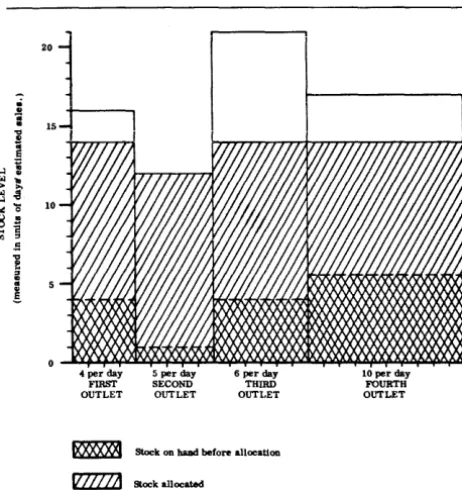
Consider a system of one production site and four retail outlets in which the four outlets have storage capacities of 64, 60, 126 and 160 items, respectively. At the start of week one, the daily sales for each are estimated as 4, 4, 7 and 10 items, respectively. It is considered that the optimum restocking level at the start of each week is 10 days' estimated sales and they are so stocked.
-items i 20 I
I Items
"
)(.)(
..A,," 'f. U :)(
X 70
~It~~S )< 40 <
~~
)< Items<~X
:i>
'Items~. y. "J:I,' X " ,X
-"
:X
.X
4 per day 4 per day FIHST SEeO:-''!) ()J.lTl ET OllTLET
7 per day TIIIHD OFTLET
~ Stock for 10 days' estimated s,dcs
c=J Unused storage capacity
X
:"
,X X XX
:X 100 <
~
Items
<
,AX ,X ' X}\
10 per day FOUHTll OllTLET
I
Diagram 1. Stock Position At Beginning Of Week 1.
Diagram 1 represents this stock position. On the horizontal axis, each outlet has a base rep-resenting one day's estimated sales and on the vertical axis, the height represents stock as a number of days' estimated sales. In this dia-gram, area is a measure of items. There are two areas shown for each outlet-occupied storage space and spare storage space. The storage capacities range between 15 and 18 days' sales. In this situation the production volume calculated for week one is 150 items, which is the total estimated week's sales with no corrections required for over- and under-stocks.
Suppose that during week one the sales are, in fact, 24, 35, 46 and 45 items, respectively. As a result of these sales, the forecasters make two changes, in which the estimated daily sales for outlets 2 and 3 are altered to 5 and 6 items. The position at the .end of week one is then shown in Diagram 2. These changes have had
20
-16~'XX8
5 Items
4 per day 5 per day FIRST SECOND OUTLET OUTLET
r"
24~Jt~ms
6 per day THIRD OUTLET
Amount of stock on hand
---. r ~
55 Items
lit per day FOURTH OUTLET
..
Diagram 2. Stock Position At End Of Week 1.
I
I
I
....l
'" ~
'" ....l
~
g 1;;
100 items to distribute. If each demand is rationed by the same factor, and allocations of two-thirds of demand are made, the new posi-tion would be as shown in Diagram 3. This
20
~
15]
E
~
..,
~
'S ., 10
'§ C "C
;
!4 per day 5 per day FIRST SECOND OUTLET OUTLET
6 per day THIRD OUTLET
~ Stock on hand before allocation
~ Stock allocated
10 per day FOURTH OUTLET
Diagram 3. Stock Position If All Demands Are
Ra-tioned Pro-rata.
would mean that the outlets had stocks of 8, 7, 8 and 8.5 days' sales, respectively. This system causes those that have been selling well to have the poorer stocks even when the forecasts have been corrected. On the other hand, the principle of equitable distribution would allot 16, 35, 24 and 25 items to the outlets, which would mean that each had a stock of 8 days' expected sales as shown in Diagram 4.
Simple Model
The Diagrams are constructed in such a way that after equitable distribution, the stocks are represented by rectangles of equal height, and a sirnple model can be used to illustrate the principle of equitable distribution. Let the Dia-grams represent a vertical cross-section of a rectangular tank in which the floor is divided into rectangular strips, perpendicular to the cross-section, one for each outlet. The widths of the strips are proportional to the rate of sales of each outlet. Solid blocks are inserted into the tank to represent the occupied storage space for each outlet. Each block fits exactly onto the strip corresponding to its outlet, and
....l
'"
~
'"
....l
~ g
1;;
20
~
] 15
i
-.,
~
'S 10
"'
c
"
C "C
;
!4 per day 5 per day FIRST SECOND OUTLET OUTLET
6 per day TtURD OUTLET
Stock on hand before allocation
Stock allocated
10 per day FOURTH OUTLET
Diagram 4. Stock Position If Distributed Equitably.
its height, therefore, measures the stock as a number of days' ex~ted sales. The tank is completed by a stepped roof whose height above the floor of the tank represents the limit of each outlet's storage capacity.
Now let the week's production be represented by a suitable volume of liquid which is poured into the tank. The liquid will find its own level, as shown in Diagram 4 for the case when the volume is 100. Diagrams 5 and 6 illustrate
20-
15-
10-4 per day 5 per day 6 per day 10 per day FIRST SECOND THIRD FOURTH OUTLET OUTLET OUTLET OUTLET
Stock on hand before allocation
Stock allocated
12 PROCEEDINGS-SPRING JOINT COMPUTER CONFERENCE, 1963
~
20
h
"
• 15
4 per day 5 per day FIRST SECOND OUTLET OUTLET
6 per day THIRD OUTLET
~ Stock on haDd before al\ocatlon
IZZZZZ2I
Stock allocatedh
10 per day FOURTH OUTLET
Diagram 6. Equitable Allocation of 240 Units..
alternative cases for production volumes of 30
and 240, respectively. Diagram 5 shows how the fourth outlet is ignored when its level of stock exceeds the equitable level, and Diagram 6 shows how the roof of the tank limits the allo-cation made to the second outlet.
Computation Procedure
The computation procedure consists of two parts: the first determines the level of equitable distribution; the second computes the appro-priate volume of production to be allocated to each outlet.
SUDDOse there are N outlets. Let the esti-mated
~
daily sales of outlet n be Sn items, the stock capacity be en days' sales, i.e., CnSn items, and the actual stocks be An days' sales, i.e., AnSn items. Now Cn and An denote thediscontinui-ties in the system and let them be ordered into a series Bi where i = 0, 1, 2, 3, . . . , im ,
where and
Bi ~ Bi
+
1Bo = O.
Now calculate Xin , which is the volume
re-quired to bring up the stock of outlet n from Bi -1 to as close to Bi as the capacity
en
ailows.If Bi -1 ~
en,
IfBi ~ AnOtherwise,
Xin = 0
Xin =
a
x
in = [min(C n, BJ- max (An, Bi-1)]8n.
Compute Fi where
. N
Fi =.~
2:
Xin .i=1 n=1
Then Fi is the volume required to bring up the stocks of all outlets to as close to Bi as the capacities allow.
Let P be the volume of production to be allocated. Then find I such that
FI ~ P ~ FH1 .
Then the level L of equitable distribution is defined by
where
Q = (P - FI)/(FH1 - FI ).
The allocation Dn for outlet n is defined by
I
Dn =
2:
X in+
QXCH1)n.i=1
These allocations have the property that their sum is exactly equal to the volume of produc-tion, because
N N
2:
Dn = FI+
Q2:
XCH1)nn=1 n=1
=
FI+
(FI+1 - F1)(P - F1)/(FH1 - FI )= P.
[image:20.618.74.305.48.293.2]Numerical Example II
Table 1 shows the values of Sn, ClI , Atl , for the
four outlets. The values of Bi are shown in Table 2, and they correspond to the discontinui-ties marked in Diagram 2. Table 3 shows the values
Xin
computed for the situation illustrated • T"'\- 0 rT1t... ... _1.".., _ _ ..f--n+nln n~" n"",...,111fl ....Hi J.Jiagrarl1 u. .1.Ut ~VIU.11111 lMIJC;U':' "'.1.0;;; ~UUH""''''
tively cross-cast at the foot to give the values Fi • Three cases are illustrated in which P (the
volume of production) is 100, 30 and 240,
respectively.
Case 1, when P = 100:
F4 = 37.5
<:
100<:
200 = F5Q =
(lao -
37.5)/(200 - 37.5) = 625/162.5= 5/13
L = 5.5
+
5(6.5)/13= 8 days' sales.
Case 2, when P = 30:
F'2 = 15
<:
30<:
37.,5 = F3Q = (30 - 15)/(37.5 - 15) 15/22.5 = 2/3 L = 4
+
1.5(2/3)Case 3, when P = 240:
F 5 = 200
<:
240<:
280 = F6Q (240 - 200)/(280 - 200)
L 12 1r 0.5(4)
14 days' sales.
Quant ity Ollt let Number Estimated Daily Sales Stock Capacity In "Days Sa les" Actual Stock In "Days Sa les"
Code
Sn c"
An
Ollt let Outlet
I 2
16 12
Discontinuity
Emp ty stockrooms
C..Jrren t leve 1 ou tIe t 2
0.5
Outlet Out let
3 4
10
2! 17
5.5
2,3 Cllrrent leve Is ou tIe t s 1 and )
BI 5.S 12 16 17 21 (Days) 5.5 12 16 17 21
Current ieve 1 ou tIe t 4 Capacity level outlet 2 Capdci ty level out let 1 Capacity level outlel 4 Capacity level outlet)
Value. of Xtn outlet 1 outlet 2 outlet 3
15 0 7.5
26 32.5 39
16 24
6 24
~Xi FI all
outlet 4 outlets 0.0 0.0 15.0 15.0 22.5 37.5 0.0 37.5 65 162.5 200.0 40 80.0 280.0 10 16.0 296.0 24.0 320.0
These cases are illustrated graphically in Diagram 8. The graph is formed by joining the pairs of points (Bi1 Fi ) computed from Table
2. By taking the value of L corresponding to
the value P on the Faxis, the same answers are obtained as when using the algebraic method given above.
400 IF
300
100
~~~~----~---+---+----~~L
10 15 20 25 DAn
Diagram 8. Quantity F Required To Raise Minimum
Stock Level to L Days' Estimated Sales.
P1'actical Cases
In practice, the procedure detailed above is not suitable for general computation. The pro-cedure suffers from the disadvantage that the determination of the series Bi is not straight-forward. In addition, it produces many more Bi values than are usually necessary for the precision required, and which increases the computing unnecessarily. With 50 outlets in the example above, there vlould be nearly 100 values of Bi • If, on the other hand, arbitrary
choices of Bi are made, the effect is to produce a graph only slightly different· from Diagram 8. Table 4 shows a possible set of Bi1 and the
Bi (Days) 12 15 18 21
Values of Xin
outlet 1 outlet 2 outlet 3 outlet 4 10
U 12
12 15 18 30
12 15 18 30
12 18 30
18 20
18
Fi
10 10
40 50
75 125 75 200
60 260 42 302 18 320
Fi that result from it. All these points are on the graph shown in Diagram 8, but their con-nection lines sometimes cut across concavities of the more accurate graph. This is shown most significantly for small values of L. Dia-gram 9 shows the precise graph as a solid line and the approximation as a broken line.
Re-working Case 2, using Table 4, gives
Q
=
(30 - 10)/(50 - 10)=
112
L
=
3+
3/2= 4.5 days' sales,
I I
F I
50 B
I
I I
I
40 I
I I I I I I
>- 30 /
!-o
/
~ I
~ I
I a
I
20 /
I / / I I I 10
~~~ __ -+ __ ~ ____ ~ __ +-__ ~ __ ~L
DAYS
Diagram 9. Enlargement of Diagram 8 Showing
but L in this context is only an approximation. It is more interesting to note that the alloca-tions that would be made are
4, 17.5, 6, and 2.5
which are very close to the preferred amounts
4, 20, 6, and 0
and would bring the stock levels up to
5, 4.5, 5, and 5.25
days' sales, with a maximum error of 0.5 days' sales. This is much better than rationing the available 30 by the fraction 30/150, which would allocate
4.8, 9.5, 7.2 and 9, giving stock levels of
6.4, 2.9, 5.2 and 6.4
days' sales respectively, in which case the sec-ond outlet is badly understocked. By setting the Bi at one-day intervals, the approximation error would be negligible.
Back-Orders
If a situation occurs where stock runs out and back-ordering is involved, then an area should be added below the horizontal axis rep-resenting the back-orders. Diagram 7 shows how 100 items would be allocated if at the end of week 1, the first outlet had 8 left, the fourth
4 per day 5 per day FIRST SECOND OUTLET OUTLET
6 per day THIRD OUTLET
~ Stock on hand before allocation
~ Stock allocated
10 per day
FOURTH OUTLET
Diagram 7. Allocation Allowing l<"or Back Orders.
outlet had 10 left, and the others had sold out, while the third outlet had taken orders for 18. Each would have its stock brought up to a level of 4 days' sales.
Negative Allocations
In some networks, transfers between outlets are permitted. These may be direct transfers, or indirect transfers by means of the distribu-tion point at the producdistribu-tion site. There is al-ways a stock limit set below which items may not be transferred. In the extreme, this is the zero stock level, but is more likely to be some emergency level of stock. Let the emergency level be one of the values of Bh say BE' Then the procedure is the same as before except that it is preceded by reducing the stock of each outlet to the level BE and increasing P by the sum of these reductions.
Indefinite Capacities
Where an outlet deals only in one kind of item, or where a bin system or special storage is required (say for gasoline or frozen foods), there are definite values that can be set for the ClI , but in many cases the value of Cn varies as
other items held in the same store are under-or over-stocked. In this situation, let there be J items considered and all the symbols used before now have an extra suffix j (j=1, 2, 3 ... J). Now values Cnj are allotted which must
conform to the restriction that when Vj is the
volume of an item j, then,
is less than the total capacity of outlet n. The values Cnj should be set at a level above which
any extra stocks would not materially decrease the chances of running out of stock.
Having allotted Cnj for all j for some outlet n,
let the storage space remaining, called the re-serve storage, be Rn measured in some unit of volume. For convenience, we consider the re-serve storage in terms of capacity to hold some item j whose volume is Vj' Then R = V 11 En.i
for any j and E nj is the reserve capacity of
outlet n in units of item j.
If Pj is greater than the total allocations
nec-essary to bring up the stock of each outlet to its Cflj , then the reserve capacities must be used,
stock. The reserve stock must be compared with the total reserve storage space which is
N
~ Enj V j for any j.
=1
If the volume of reserve stocks for all items together exceeds reserve storage space, the values of Pj must be reduced by some system
until it is the case. Let Hj be the fraction of
total reserve storage required by the reserve stock of item j. Then, where reserve stock exists, each outlet is filled to capacity Cnj and
then allocated a sufficient amount to bring its reserve holding to Hj Enj •
Computer Considerations
There are five major factors to be considered: 1. Volume of computation.
2. Complexity of computation. 3. Scans of the data.
4. Random or serial access to data. 5. Accuracy and rounding errors.
The volume of computation depends upon the number of outlets and the number of points Bi •
The more Bi points there are, the greater the precision of the result in general. For any given degree of precision, an arrangement of Bi in exponential steps minimizes the number of Bi •
The procedure requires scans through the data to:
1. Establish the values of Bi • This scan can
be saved if preset values are used. 2. Compute the values of Fi , and then
deter-mine L.
3. Compute the individual allocations Dn. Thus there are either 2 or 3 scans, depend-ing upon the method of establishdepend-ing the values of Bi •
If the data for the outlets can be held in a random access store, the scan to determine L
can be made by computing each Fi in turn until the allocation total P is reached. A more sophis-ticated procedure is to estimate I and arrange a searching procedure. More frequently, the data may have to be held in a serial access store. In this case, the procedure is to calculate all the Xin for each n in turn and accumulate
N
~ X in for each i. n=1
Then at the end of the scan, the values Fi can be formed.
Although the computation of Fi may be made in basic items, allocations Dn may have to be rounded to some multiple of a delivery unit. When this unit is not small compared with the smaller values of D,., the round-off procedure needs care. Any errors introduced by rounding are additional to those arising from the choice of the set of Hi' Rounding cannot be carried out indiscriminately or the sum of Dn may not equal P. If independent rounding procedures are carried out for each outlet, it is wise to group the outlets with larger Sn at the end of the scan where cumulative round-off errors can
be absorbed with least inequity. If such re-grouping is not desirable, the technique of carrying the round-off quantity into the com-putation of the next ,outlet can be used. For example, suppose Dn be rounded to D' nand D' n - Dn = dn then D'n+l is computed by rounding
off (Dn+l - dn ). This process minimizes the
cumulative round-off error at any time, and each D' n may have an error of up to one delivery
unit.
CONCLUSION
There are five major advantages that can be cited for the use of the principle of equitable distribution that has been discussed in this paper.
First, the basis of the principle is simple to understand; therefore, it is easy to explain to all employees concerned with distribution.
Second, the principle works just as easily in times of crises as in easier times. During poten-tial crises-heat-waves, blizzards, or failures in production or raw materials-supplies are ra-tioned with little fuss. During inventory build-up to minimize a future potential crisis, the surplus is shared simply and effectively.
Third, the principle is easy to mechanize and fits well into automatic data processing and simpler systems.
Fourth, the principle can be extended to cover more complex situations where several levels of inventory or sources of supply are involved.
can be used to forecast sales. From sales pat-terns and production costings, mathematical analysis4 • 5 can be used to determine optimum inventory levels and re-ordering rules. From current stocks and . ~ales forecasts, production plans can be made; then, when production occurs, equitable distribution can be made.
ACKNOWLEDGMENTS
The author wishes to thank Mr. T. R. Thomp-son of LEO Computers, Ltd., and the staff of A UERBACH Corporation for their help and encouragement in the preparation of this paper.
REFERENCES
1., BROWN, ROBERT G. (1956) Exponential Smoothing for Predicting Demand. Cam-bridge, Mass., Arthur D. Little, Inc.
2. HOLT, CHARLES C. (1957) Forecasting Seasonals and Trends by Exponentially Weighted Averages. Pittsburgh, Pa., Car-negie Institute of Technology.
3. MUIR, ANDREW (1958) Automatic Sales Forecasting. The Computer Journal, Vol. 1, p. 113.
4. WHITIN, T. M., YOUNG, J.