Developments in dynamic field gradient focusing: microfluidics and integration

(1)

Developments in

Dynamic Field Gradient Focusing:

Microfluidics and Integration

Thesis submitted in accordance with the requirements of the

University of Liverpool for the degree of Doctor in Philosophy

by

Thomas Robert Wray

(2)

i

Acknowledgements

I would like to express my thanks to my supervisor Professor Peter Myers for his

excellent guidance and ideas throughout this project and most importantly for all of

the real ale and granting me the opportunity to undertake this project.

Thanks are also extended to all the members of the Myers group particularly fellow

PhD student Dr Kevin Skinley for making the lab a great place to work.

I would also like to thank Thermo Fisher Scientific for sponsoring the DTA awards

and providing funding for this research through Dr Harold Ritchie. Thanks also go

to Pfizer for providing further funding through Dr Melissa Hannah-Brown.

I also thank all of the staff within the University Of Liverpool Department Of

Chemistry for any support over all of my time studying here.

For collaborations during the project I would like to thank Dr Tony Edge and his

team from Thermo Fisher Scientific and Dr Jetinder Singh and David Atkinson from

the University Of Liverpool Department Of Engineering.

I am grateful to my family for all of their support and understanding during all of

my studies. A big thanks to all my friends, especially everyone at the BKJJA, for all

of their enduring encouragement.

Special thanks go to my partner Kate for all of her continued support and always

being there for me, helping me through the hard times and making the good times

the best. Thanks to Kate, I have got to where I am now which I couldn’t have done

(3)

ii

Developments in

Dynamic Field Gradient Focusing:

Microfluidics and Integration

Abstract

By Thomas Robert Wray,

University of Liverpool, August 2012

Advances in modern science require the development of more robust and improved

systems for electroseparations in chromatography. In response, the progress of a

new analytical platform is discussed. DFGF (Dynamic Field Gradient Focusing) is a

separation technique, first described in 1998, which exploits the differences in

electrophoretic mobility and hydrodynamic area of analytes to result in separation.

This is achieved by taking a channel and applying a hydrodynamic flow in one

direction and a counteracting electric field gradient acting in the opposite direction,

resulting in analytes reaching a focal point according to their electrophoretic

mobility.

Work through this project has seen innovations to improve existing DFGF devices,

including the design and manufacture of a novel packing material, while

developing the latest DFGF system. This incorporates a microfluidic separation

channel, eliminating the need for packing material or monolith. The new

microfluidic device also features whole-on-column UV detection. Improvements

through the developments of this device are discussed, most notably the utilisation

of a new rapid prototyping technique. Examples of applications undertaken with

the new device are demonstrated including novel samples and integration with

(4)

iii

List of Tables

Table 1.1. Summary of the properties of purification techniques utilised for proteins. 4

Table 2.3.1. Kaleidoscope Pre-Stained Standards Test Mixture. 40

Table 2.3.2. Voltage profile for Kaleidoscope separation in figure 2.3.8. 45

Table 2.4.1. Summary of voltage profiles used to separate 40µL Kaleidoscope mixture. 50

Table 2.4.2. EFG and flow rates applied to separate the Kaleidoscope mixture in figure 2.4.5.

54

Table 2.6.2. Particles manufactured using the hand spray and pneumatic spray. 63

Table 2.6.3. EFG Applied to separate the mixture of BPB and AM. 76

Table 2.6.4. Experimental conditions applied to the device to separate the Kaleidoscope test mixture with the monodispersed packing material.

79

Table 3.3.1. Summary of conditions for a microfluidic DFGF test separation of BPB and AM.

98

Table 3.3.2. Conditions for the separation of BPB, AM and AY in figure 3.3.9. 105

Table 3.3.3. Conditions used to result in the focusing of the 3 component mixture of AM and BPB and Acid Yellow.

109

Table 3.3.4. Experimental parameters for the separation of 5µL of 10% BPB AM and AY test mixture.

112

Table 3.3.5. Conditions for the separation of the Bio-Rad Kaleidoscope Pre-stain Standards in figure3.3.16.

120

Table 3.3.6. Conditions used to separate AM and BPB testing the 200µm electrode channel.

136

Table 3.3.7. Optimised Microfluidic DFGF device. 138

(9)

viii Table 3.3.9. Table of voltage profiles and flow rates for the repeat separation of the

kaleidoscope test mixture using the optimised microfluidic DFGF.

142

Table 3.3.10. Summary of controlling parameters and features available in data acquisition from the PDA using the bespoke software.

144

Table 3.3.11. Optimum PDA Detection parameter using the LCD backlight. 149

Table 3.3.12. Separation of the kaleidoscope mixture detected with the PDA detectorin

figure 3.3.35.

150

Table 3.3.13. UV light source stability issues. 154

Table 4.2.1. Voltage profiles and flow rates applied to separate the functionalised GNPs. 162

Table 4.2.2. Parameters used in separating the GNPs in the microfluidic DFGF. 168

Table 4.3.1. Optimal conditions for detection by C4_{Dfromthe profiling for BPB.} ₁₇₃

Table 4.3.2. Changes in EFG for the separation of AM and BPBin figure 4.3.8. 182

Table 4.3.3. Conditions for the separation of AM and BPB monitored by C4_{D and UV.}

The detection data is shown in figure4.3.9.

184

Table 4.3.4. Conditions for repeat separation of the Kaleidoscope proteins in figure 4.3.11.

187

Table 4.4.1. Timings for the application of the EFG in the microfluidic device during 2D method.

(10)

ix

List of Figures

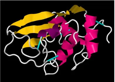
Figure 1.1.1. Protein structure of Lysozyme. 3

Figure 1.2.1. Configuration of the EFGF device. 13

Figure 2.1.1. Theoretical model for DFGF. 19

Equation 2.1.1. The Flux equation. 19

Equation 2.1.2. The flux equation solved for C, where Mi is the total number of moles

of analyte.

19

Equation 2.1.3. Χi defines a point along the length of the separation channel where an

analyte will come into focus.

20

Equation 2.1.4. Variance of the width of a focused band of analyte. 20

Figure 2.2.1. DFGF Set Up and supporting equipment. 21

Figure 2.2.2. DFGF Channel Configuration. 22

Figure 2.2.3. DFGF packing apparatus. 24

Figure 2.2.4. Flux Instruments Rheos Janeiro 3.0 software. 26

Figure 2.2.5. Protasis Power supply schematic. 27

Figure 2.2.6. Protasis UController HV Control Software. 28

Figure 2.2.7. An example of a linear EFG generated by the Labview Protasis Ucontroller software in Automatic Mode.

(11)

x Figure 2.2.8. An example of the EFGs which can be applied by the Labview

Ucontroller software in Manual Mode.

30

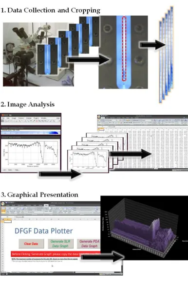
Figure 2.2.9. A) Nikon D80 with a 60mm 1:2.8D macro lens configured to take images of the separation channel with the addition of a LED ring illuminator. B) Nikon Camera Control Pro software user interface.

31

Figure 2.2.10. A) Detection using GIMP to subtract images highlighting any changes in the positions of analytes with a corresponding profile measurement. B) Next a

profile plot is generated using ImageJ, in this instance, FIJI16_{, a rich featured version}

of ImageJ.

32

Figure 2.2.11. 1) Data Interpretation. 2) The cropped image stack is loaded into ImageJ and all the profiles are measured. 3) This data was loaded into the MS Excel ‘Profile Generator’ producing a graph of the separation.

34

Figure 2.3.1. Structure of Bromophenol Blue (BPB) 4,4'-(1,1-dioxido-3H-2,1-benzoxathiole-3,3-diyl)bis(2,6-dibromophenol).

35

Figure 2.3.2. Structure of Amaranth (AM) trisodium (4E)-3-oxo-4-[(4-sulfonato-1-naphthyl)hydrazono]naphthalene-2,7-disulfonate.

36

Figure 2.3.3. Separation and focusing of Bromophenol Blue (BPB) and Amaranth (AM).

37

Figure 2.3.4. Injection of BPB with a static linear EFG. 38

Figure 2.3.5. BPB focusing as shown in the form of a Montage. Constructed by taking the cropped images and stacking them in order.

39

Figure 2.3.6. Kaleidoscope bands migrating back and forth along the separation channel in a focused band of the protein mixture.

41

Figure 2.3.7. A) Graphical representation of kaleidoscope mixture focused in the first gen. device. B) Montage of the images displaying the movement of the bands along the separation channel.

42

Figure 2.3.8. A) ‘Run1’ From Table2.3.2 Displaying the kaleidoscope test mixture being manipulated in the separation channel. B) ‘Run2’ From Table2.3.2 An immediate follow up experiment injecting the sample and focusing again. Three separated bands can be seen in the plot.

46

(12)

xi Figure 2.4.2. More than 20µL of 10%v/v Lissamine green solution being injected and

focused into a tight band.

48

Figure 2.4.3. A mixture of Amaranth and BPB separated and focused. 49

Figure 2.4.4. A) Graphical representation of the separation of 40µL Kaleidoscope mixture. B) Single plot at 147mins displaying at least four bands.

51

Figure 2.4.5. The separation of Kaleidoscope test mixture displayed graphically. Five component peaks are observed during the separation.

54

Figure 2.5.1. LEFT: Displays the Protasis device. RIGHT: top area of separation channel with the blemishing of the acrylic after running at the maximum 1000V without cooling.

57

Figure 2.5.2.Optical Microscope image of polyacrylamide packing material in DFGF channel. Void spaces and irregular interstitial spacing are visible across the entire bed.

58

Figure 2.5.3. Left to right, images displaying a bed rearrangement leading to the collapse of the membrane.

59

Figure 2.6.1. Drop generator system. 62

Figure 2.6.2. Printer Head of the Domino printer. 65

Figure 2.6.3. Optimal ‘Break Up’ of droplets from the spray head on the Domino printer.

66

Figure 2.6.4. Spraying monodispersed particles using the modified Domino printer. 67

Figure 2.6.5. Mercury Porosimetry of the 80µm silica particles. 68

Figure 2.6.6. SEM images of the drop by drop 80µm silica particles. 69

Figure 2.6.7. Optical microscopy of the packed GC column. 70

Figure 2.6.8. GC separation of Petroleum Ether and DCM at 60°C using the 1.2m column packed with 80µm silica.

(13)

xii Figure 2.6.9. FTIR analysis of the 80µm particles before and after treatment at

1000°C.

72

Figure 2.6.10. First Gen. DFGF packed with 80µm porous silica particles. 73

Figure 2.6.11. A) Graphical representation of a flow through of 10% BPB AM

mixture at 1µLmin-1_{. B) Montage of images displaying the mixture as purple in}

colour, showing no derivation of red or blue corresponding to BPB or AM.

75

Figure 2.6.12. Separation of BPB and AM in a faster time utilising the larger pore monodispersed packing material.

77

Figure 2.6.13. A) Graph of the separation of the Kaleidoscope test mixture. B) Montage of the Kaleidoscope separation.

80

Figure 3.2.1. Initial design of a microfluidic DFGF from Dolomite. 89

Figure 3.2.2. Design of the Microfluidic DFGF separation channel chip and electrode chip.

90

Figure 3.2.3. Microfluidic DFGF device exploded view. 91

Figure 3.2.4. Microfluidic DFGF device design summary. 93

Figure 3.3.1. Prototype Electrode connector made from IDC connector. 94

Figure 3.3.2. A) Microfluidic DFGF Electrode Connector. B) Connector inserted in the recess at the back of the microfluidic DFGF. C) All HV connections in place using IDC connectors.

95

Figure 3.3.3. Dolomite User Guide for the microfluidic DFGF. 96

Figure 3.3.4. Initial Separation of BPB and AM with the microfluidic DFGF. 99

Figure 3.3.5. Severe degradation of the platinum electrodes on the microfluidic DFGF electrode chip.

100

(14)

xiii

Figure 3.3.7. Gold electrode array on an existing electrode chip. 102

Figure 3.3.8. Completed gold electrode array and chip holder base with fixed connector.

103

Figure 3.3.9. The molecular structure of Acid Yellow, Disodium 2,5-dichloro-4-[3-methyl-5-oxo-4-(4-sulfonatophenyl)diazenyl-4H-pyrazol-1-yl]benzenesulfonate.

104

Figure 3.3.10. Separation and focusing of BPB, AM and AY. 107

Figure 3.3.11. A) Graphical representation of the focusing of the 3 component mixture of AM and BPB and Acid Yellow. B) Image of the separation channel of the focused band where it is apparent that some of the sample has leaked from the separation channel.

110

Figure 3.3.12. Graph showing the separation and focusing of a 5µL injection of the BPB AM and AY.

113

Figure 3.3.13. Membrane from experiment in figure 3.3.11. 114

Figure 3.3.14. Enlarged cross section of the microfluidic DFGF detailing the issue with the channel dimensions and leakage issue.

116

Figure 3.3.15. Prototype Teflon insert to provide a narrower electrode channel and better support for the membrane in comparison to the original PEEK electrode channel and gasket.

117

Figure 3.3.16. Prototype Platinum Electrodes on a plastic chip with holes drilled for the flow of electrode channel buffer and an IDC connector to interface with the Protasis Power Supply.

118

Figure 3.3.17. Separation and focusing of the Bio-Rad Kaleidoscope test mixture in the microfluidic DFGF using the prototype platinum electrode array and prototype Teflon electrode channel.

121

Figure 3.3.18. Schematic displaying the setup of Stereolithography Apparatus. 123

Figure 3.3.19. Electrode chip mask design drawn in CAD software. 125

(15)

xiv

Figure 3.3.21. Decomposed PVD electrodes after 20mins at 200Vcm-2_. ₁₂₇

Figure 3.3.22. Final Electrode chip. Houses five platinum electrodes on a glass chip with IDC connector.

127

Figure 3.3.23. A, B & C) ‘Gasket Holder’ drawn in CAD ready for SLA manufacture. Top, Base, and Front elevations respectively. D) Manufacture of ‘Gasket Holder’ using SLA RP.

128

Figure 3.3.24. Cross section schematics of the ‘Gasket Holder’ with channel widths of 100µm and 200µm respectively.

130

Figure 3.3.25. A) This graph displays the need to collect images at a shorter time intervals as the analyte comes into focus seemingly instantaneously where this effect in actual is a gradual phenomenon. B) The montage also displays this as the AM and BPB are observed.

132

Figure 3.3.26. Separation of BPB and AM using 100µm electrode channel. 133

Figure 3.3.27. Graph of separation using the 200µm electrode channel. 136

Figure 3.3.28. Separation of Kaleidoscope test mixture displaying a region of focused proteins.

140

Figure 3.3.29. Separation of the kaleidoscope test mixture using the optimised microfluidic DFGF with enhanced imaging.

142

Figure 3.3.30. Toshiba TC101 PDA Detector. 144

Figure 3.3.31. PDA Software user interface with option to collect single samples or collect a sequence which are stored in the capture buffer before writing to a *.CSV file.

144

Figure 3.3.32. PDA DFGF configuration using ambient light. Left: Image illustrates the setup. Right: Cross section of the chip and the PDA.

145

Figure 3.3.33. PDA detector graph showing three peaks corresponding to the three markers on the separation channel.

146

Figure 3.3.34. PDA Light sources. 148

(16)

xv Figure 3.3.36. Test displaying the introduction of a Test mixture into the separation

channel.

152

Figure 4.2.1. CPS Analysis of the functionalised GNPs. 160

Figure 4.2.2. Graphical representation and Montage of the separation of the functionalised GNPs in the first gen. DFGF device.

163

Figure 4.2.3. SEM of the packing material from the band 40mm along the channel displaying singular GNPs on the surface of the polyacrylamide spheres.

164

Figure 4.2.4. SEM of the packing material from the band 55mm along the channel displaying aggregates of the GNPs on the surface of the polyacrylamide spheres.

165

Figure 4.2.5. Graphical representation of the open channel microfluidic DFGF separation of the GNPs.

168

Figure 4.2.6. Image of the separation channel with the GNP’s separated from the aggregates.

169

Figure 4.3.1. UV and C4_{D set up.} ₁₇₂

Figure 4.3.2. Profile of condition for C4_{D detection of BPB.} ₁₇₃

Figure 4.3.3. Labview DAQ System for C4_{D and UV detectors.} ₁₇₄

Figure 4.3.4. The first data successfully collected from the DAQ system showing a flat base line for each detector.

175

Figure 4.3.5. Graphical representation of the whole column reflectance data displaying the BPB moving through the microfluidic DFGF.

177

Figure 4.3.6. BPB injected and brought into focus and detected. 178

Figure 4.3.7. Elution detection from the microfluidic DFGF separation of AM and BPB.

179

Figure 4.3.8. Separation of AM and BPB with post column detection. 183

Figure 4.3.9. Separation of AM and BPB over three injection with C4_{D and UV}

detection.

(17)

xvi Figure 4.3.10. Post separation channel detection for the separation of kaleidoscope test

mixture in chapter three figure3.3.28.

185

Figure 4.3.11. Graph displaying the PDA data for the separation of the kaleidoscope

test mixture with C4_{D and UV detection.}

188

Figure 4.3.12. Post separation channel detection for the separation of the Kaleidoscope test mixture described in chapter three figure33.34.

190

Figure 4.4.1. HPLC-DFGF-MS Set up. 193

Figure 4.4.2. Injection of insulin pumped at 100uLmin-1_{without applied electric field.} ₁₉₄

Figure 4.4.3. Injection of insulin pumped at 100uLmin-1_{with the electric field applied}

between 1min and 6.5min with 1000V on each electrode.

195

Figure 4.4.4. Overlaid chromatograms from the test injection of insulin with and without the use of the electric field.

195

Figure 4.4.5. Injection and flow through of the sample without a column at 2μLm-1

with no electric field applied.

197

Figure 4.4.6. Injection and flow through of the sample without a column at 2μLm-1

with an electric field applied from 0mins until the end of the run.

197

Figure 4.4.7. Overlaid chromatograms for focusing effect without a column in place. 198

Figure 4.4.8. Integration of the microfluidic DFGF with a 2D HPLC valve switching array.

199

Figure 4.4.9. Switching valve positions and flow of sample for the DFGF assisted 2D HPLC procedure.

202

Figure 4.4.10. The DFGF assisted 2D HPLC procedure running without the use of the EFG for comparison.

203

Figure 4.4.11. Chromatogram from the DFGF assisted 2D HPLC separation with the EFG in operation.

204

Figure 4.4.12. Overlaid chromatograms from the DFGF assisted 2D HPLC separations with and without the pre-concentration of the electric field.

205

(18)

(19)

1

Chapter

1

. Introduction

1.1 Background

Advancements in cellular research and the completion of the human genome

project have driven the demand on the analysis of biomacromolecules to reach a

point outstretching current abilities. As the coding of human and other genomes

are now understood, the next step is to identify and characterise specific proteins

and determine which processes and pathways regulate their production at a cellular

level. For the last decade many chromatographic techniques have been extensively

developed but still fail to deliver the efficiency and selectivity required for

separations and purification of proteins in the areas of biological, medical and

physical sciences. This can be attributed to proteins themselves being a challenging

matrix for separation.

Proteins are the most abundant macromolecules occurring naturally. These

macromolecules range from small peptides to massive polymers and are found in

thousands of diverse forms. These varieties of proteins, regardless of origin, are

made up from the same twenty standard amino acids. Despite twenty fundamental

building blocks the range of proteins and their application in organisms is vast.

From the silk from spiders, feathers of a bird, poisons in mushrooms, to more

specific and novel proteins namely Enzymes. Enzymes, all of which being proteins,

are the most diverse and specialised1_.

There are twenty amino acid components which are composed of a primary amine

(-NH3+), a carboxylic acid (-COOH) group bonded to a central alpha carbon, and a

(20)

2 However, there is one exception to this general structure, namely proline, which has

a secondary cyclic amine and is therefore characterised as an imino acid2_{. A protein}

itself is formed by linking different combinations of these side chains by a covalent

peptide bond formed between the amino group of one, and the alpha carbon of the

next amino acid. This gives proteins their characteristic of having a rigid back bone,

from planner peptide groups, and suspended side chains.

As a result of this complicated macromolecular arrangement, a proteins structure is

described in terms of four levels of intricacy1_{. The primary structure of a protein is}

the linear chain of amino acids linked by the covalent peptide bonds. Also included

in the primary structure are other covalent bonds such as disulphide bonds from

cysteine residues that are in close proximity but not part of the linear chain.

The secondary protein structure is dependent on the nature of ‘folding’ within

sections of the polypeptide chain. Protein folding is a rearrangement in space of the

polypeptide structure into a lower energy conformation.

There are two common types of folding, α-helix and β-pleated sheets. The

formation of an α-helix is a result of the carbonyl oxygen of each peptide bond

hydrogen bonding to the hydrogen of the amino group of the amino acid four units

along the chain. These bonds run parallel to the axis of helix and depending on the

interactions of the amino acid R-groups this conformation can be stabilised or

destabilised. The β-pleated sheets occur where polypeptide bonds, from the same

chain or different chains, have hydrogen bonds between them. This bonding is

planer and has a slight twist which in some cases can result in a β-barrel2_.

The tertiary structural elements of proteins refer to the three-dimensional

(21)

3 For example, when introduced to water, a protein will fold as to expose the

hydrophilic elements of the chain and protect the hydrophobic species.

Interestingly, once the protein has folded in its natural media it is held in place by

electrostatic interaction of the side chains and by hydrogen bonding with the

disulphides.

Quaternary protein structures are where proteins are made up of more than one

polypeptide chains. This therefore refers to the spatial arrangement of different

[image:21.595.123.517.347.628.2]

polypeptide units and the interactions between them.

(22)

4 1.2 Separation of Proteins

These different elements of the proteins structure generate a number of properties

which can be exploited to result in successful and efficient separations and

purification. A summary of the most common methods of purification techniques

and the properties exploited are listed in table 1.1 below.

Technique Property

Exploited Capacity Resolution Yield Cost

pH

precipitation Charge High Very Low Medium Low

Ammonium sulphate precipitation

Hydrophobicity High Very Low High Low

Aq. Two phase extraction

Mixture,

Bip-Affinity High Very Low High Low

Ion exchange

chromatography Charge Medium Medium Medium Medium

Hydrophobic interaction chromatography

Hydrophobicity Medium Medium Medium Medium

Isoelectric

focusing Charge/ pI Low High Medium High

Dye Affinity

chromatography Mixture Medium High Medium Medium

Ligand affinity

chromatography Bio-Activity

Medium-

Low Very High Low High

Size Exclusion

Chromatography Size

Very

Low Low High Medium

Table 1.1. Summary of the properties of purification techniques utilised for proteins3_.

Common procedures for the purification of proteins will include a number of steps

(23)

5 Initially, the most important factors are a high capacity and low cost to yield the

highest volume of protein from its source.

After this, or additional steps, the resolution is most important to enable the

determination and identification of individual proteins from a complex mixture.

There are many existing methods for a range of separation techniques which are

applicable to proteins. These can be described as two types of technique. Firstly,

chromatographic techniques where separation occurs by partitioning between the

mobile and stationary phase. Secondly, electrophoretic separations where electric

fields are used to mobilise individual proteins to unique points within a gel or

channel.

1.2.1 Chromatographic Protein Separation Techniques

The most effective and commonly used chromatographic separation techniques

include Size Exclusion, Ion Exchange, Affinity chromatography, High Performance

Liquid Chromatography and Liquid Chromatography Mass Spectrometry

(LC/MS)4_.

Size Exclusion Chromatography (SEC), or gel filtration, exploits the differences in

the overall size of proteins to result in separation5_{. This is achieved by packing a}

column with a porous spherical insoluble polymer particle, typically porous

polyacrylamide beads, and pumping the sample through this packed bed. This

packing results in a range of pathways through the column. Smaller species and

small impurities flow through the column and diffuse in and out of the pores and

(24)

6 Larger species, i.e. the desired proteins, are too large to flow through the pores of

the packing material and flow through the column following a path only through

the interstitial space and elute from the column faster. As shown in table 1.1 size

exclusion is a low resolution and low capacity technique.

Ion Exchange Chromatography separates proteins according to net charge. Anion

exchange utilises a positively charged stationary phase packed into a column6,7_{. A}

protein sample is introduced and pumped through the column by the mobile phase,

typically buffered solution at pH 7. The result of this is that any proteins with a

negative charge will have bound to the stationary phase and any neutral or

positively charged species will have passed straight through the column. To elute

the negatively charged species, the mobile phase is changed from a buffer solution

to a salt solution of NaCl. The chloride ions then outcompete the protein for

charged sites on the stationary phase resulting in displacement and elution. Cation

exchange is the opposite, running a negatively charged stationary phase. Elution

can be controlled in both polarities by changing the pH of the buffer solution

resulting in changes to the net charge of the proteins. Ion Exchange provides a

separation technique which can deliver separation of large mixtures; however the

reproducibility of separations using these columns is poor due to the differences in

efficiency of ligand coverage over the stationary phase and packing of the charged

material being difficult.

Affinity Chromatography, AC, utilises the binding specificities of a given protein to

another molecule, the ligand, to result in separation 8,9_{. Once a suitable ligand has}

been identified to function as a binding site, it is covalently bonded to the stationary

(25)

7 Next a sample mixture containing the desired protein is mobilised through the

column with mobile phase favouring the conditions for absorption of the protein to

the ligand. Only the specific desired protein will interact with the carefully chosen

ligand and the other undesired proteins and impurities are flushed out of the

column. To elute the desired protein the mobile phase is changed to favour

desorption and the protein is collected in high purity.

Despite the high resolution there are difficulties in scale up of this separation

technique. Most importantly AC is a highly labour intensive and costly approach

because of the work involved in identifying and creating a specific stationary phase,

as a result this process is more commonly used in areas such as pharmaceuticals

were purity is considered paramount and far outweighs the cost.

High Performance Liquid Chromatography, HPLC, utilises high pressure pumps

and smaller particle sizes to increase the migration of samples through a column10_.

The decrease in particle size facilitates faster separations by increasing the surface

area of the stationary phase and providing a shorter diffusion pathway through the

particles. This results in the ability to operate at higher flow rates further increasing

the speed of separation and reducing the diffusion of samples11_.

Reverse Phase High Performance Liquid Chromatography, RP-HPLC, separates

analytes according to differences in hydrophobic interaction. A functionalised

hydrophobic stationary phase is packed into the column and a polar mobile phase is

passed through at high pressure. Conversely ‘Normal Phase’ HPLC consists of the

opposite, with a polar stationary phase and non-polar mobile phase, the separation

occurs as a result of the sample having an affinity to the mobile or stationary

(26)

8 RP-HPLC is preferred for the analysis of proteins and biological samples as the

resolution is very high, facilitating the separation of polypeptides of the same mass

with differing sequences. Furthermore the aqueous mobile phase used in RP-HPLC

is more compatible with biological samples compared to the high organic content

used for Normal Phase HPLC. For larger polypeptides and, even larger proteins,

the retention mechanism in RP-HPLC differs from that of smaller molecules. When

smaller molecules flow through the column the species are constantly partitioning

between the mobile and stationary phase.

Yet proteins and polypeptides are too large to continually partition and simply

absorb to the hydrophobic surface of the stationary phase until the concentration of

organic modifier in the mobile phase is increased to reach a critical point which

causes desorption12_{. At this point the species flows through the column with}

minimal interaction with the stationary phase. Though this technique provides

separations with good resolution, there are shortcomings with the ability of the

technique to handle complex samples. Furthermore the protein sample will often

be denatured in RP-HPLC conditions removing any biological activity of recovered

protein13_.

To overcome the issue of sample complexity a second dimension of separation can

be added before separation by RP-HPLC. Two Dimensional HPLC, 2D-HPLC,

introduces an Ion Exchange column to fractionate the sample before further

separation by RP-HPLC, improving the resolution and selectivity of separations by

combining retention mechanisms14–18_{. Where 2D-HPLC is implemented, Mass}

Spectrometry is the de-facto detection method falling under the category of Liquid

(27)

9 LC/MS is a powerful tool in protein characterisation as the molecular weight of a

given sample is determined while also deciphering sequence information by the

detected mass fragements4,14_{. As the MS provides an increase in resolving power}

and reduced analysis time, separations can be run in less time, making MS more

favourable than other detection methods such as refractive index or UV detection.

1.2.2 Electrophoretic Protein Separation Techniques

The most widely used electrophoretic separation techniques include; 2D Gel

-Electrophoresis Mass Spectrometry (2-DGE/MS)19_{, and Capillary Electrophoresis}

Mass Spectrometry (CE/MS)20_{. Commercial instrumentation has been developed}

for CE/MS, LC/MS and GE/MS21_{. The most widely implemented technique}

appears to be 2-DGE/MS4_{. This is due to this method facilitating the separation of}

different proteins yielding sufficient quantities for further analysis.

State-of-the-art 2-D gel operations use precision robotics to dissect the gels, enabling

the bands of protein to be analysed further by mass spectrometry. Having run an

electrophoretic separation by applying an electric field over a polyacrylamide gel,

migrations of individual proteins form bands at different lengths along the gel.

These bands are then fed into optical readers and analysed by a computer to give a

chromatogram, before being further analysed by MS. This process can sample

thousands of proteins a day, but in spite of this, it can still take months to determine

the proteins native structural elements. It is fundamental that in proteome research

proteins from cells and tissues need to be isolated in high purity and quantity for

(28)

10 Chromatography and electrophoresis are most extensively used in high-resolution

purification22,23_{. As a result work has been conducted to combine these techniques}

in hope of devising a hybrid of the advantages of both24_.

Electroseparation methods have long been required and developed, but with the

complexity of Isotachophoresis (ITP), the sample limitations of Capillary

Electrophoresis (CE) and the mobile phase and support problems in Capillary

Electrokinetic Chromatography (CEC), High Performance Liquid Chromatography

(HPLC) is still the major liquid separation technique. This is despite the major

problems and limitations in the analysis time and resolution, e.g. chiral

separations25–27_{, and isoform fractionation}28_{. Therefore alternative methods and}

instrumentation are needed. Research has continued on the combined development

of these electrophoretic techniques by combining the new developments of;

microfabrication, detection, and computer controlled fluidics and voltages. This has

seen new electrophoretic techniques emerge that remove key disadvantages of the

individual techniques. These techniques are known as electro- chromatography

(EC)24_{. The most recent advancements utilise electrophoretic mobilisation at the}

same time as a hydrodynamic flow making these focusing techniques. Advances in

this area began with Counteracting Chromatographic Electrophoresis (CACE)29_.

1.2.3 Electrofocusing Techniques

In CACE, different grades of chromatographic media are setup up in the direction

of flow. Simultaneously an electric field is applied in the opposing direction to the

mobile phase. This field can then be manipulated to counteract the hydrodynamic

(29)

11 This work by O'Farrell et al.29_{focused proteins into bands using an electric field,} without the use of a pH gradient. However, this method of separation showed poor

performance with mixtures of proteins and had issues with scale up30_.

Comparing electrofocusing techniques described above with CE, the performance is

similar. However, the gains made in complex and costly modifications to CE are

inherently encompassed in electrofocusing technologies. This introduces significant

advantages for challenging analytical separations, providing high resolution and

high concentration of samples, lending itself to small scale applications31_{. Isoelectric}

focusing (IEF) however enables scale up at the cost of large increases in time for

separations to occur.

IEF is a form of zone electrophoresis which separates analytes across a static pH

gradient resulting in separation according to isoelectric point. Though IEF offers

very high resolution, it has inherent problems with the complexity of stabilising the

pH gradient under running conditions, particularly at preparative and large scales.

At the isoelectric point (pI), many samples become insoluble. Furthermore some

groups of samples are unable to be focused by this method either because

degradation occurs at their isoelectric point; for example, nucleic acids. Moreover,

IEF is a batch technique which is analogous to other chromatographic techniques

presenting difficulties in implementing a continuous flow system. In addition to

these issues the ampholytes which are key to stabilising the pH gradient, contribute

a high cost to the recovery of protein purified to the cost of focusing30_.

Flow counterbalanced capillary electrophoresis (FCCE)32_{developed by Jorgenson}_et

al. provides separation by CE. The difference with this approach is that a counter

(30)

12 The effect of the this counteracting flow is that the separation occurs more gradually

over the length of the capillary which has the same effect as increasing the length of

the column. Improvements in resolution and efficiency of a given CE separation

were demonstrated by using FCCE without modification of the buffer, field

strength, or method of detection.

Even though there are two opposing forces within the capillary, this is not a true

focusing device as the analytes do not become stationary at any point in the

separation. To fully concentrate a desired protein the opposing forces must control

the flow movement of the species in both directions.

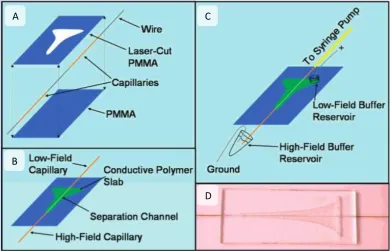
Electric Field Gradient Focusing, EFGF, described by Lee et al.33,34_{, is a true} electrofocusing technique. A capillary is placed inside a secondary reservoir

constructed from a conductive polymer. The configuration of the EFGF device is

shown in figure 1.2.1. As a hydrodynamic flow is applied in one direction through

the capillary, an electrokinetic force is applied in the secondary reservoir acting in

the opposite direction. The conductive polymer allows the propagation of the

electric field, but not the sample. This results in analytes reaching focal points at

(31)

13 Figure 1.2.1. Configuration of the EFGF device. A) Exploded view of components made from Poly(methyl methacrylate), (PMMA). B) Assembled device. C) Assembled device with buffer reservoirs. D) Image of actual EFGF device.

It is noted that this is a static electric field gradient acting across the full length of

the device. This configuration allows for the separation of analytes; however the

electric field either retains all of the samples or allows them to elute. To solve this

issue and facilitate the stacking of a concentrated sample, a tandem EFGF was

redeveloped to isolate and re-focus a target protein once separated from a matrix35_.

Further work on EFGF saw the evaluation of the influence of the hydrogel used to

form the channels36_{. This work raised questions over the shape of the reservoir}

channel which was later changed to facilitate a more stable electric field.

Improvements to this system saw the use of polyethylene glyocol for the

construction of the reservoir and therefore an increase in the effectiveness of the

electric field propagation37_. A

B

C

[image:31.595.124.516.73.324.2]

(32)

14

Key observations were made in a theoretical study38_{which indicated that the shape}

of the channel had a direct effect on the propagation of the electric field. A bi-linear

EFGF39_{was developed which is a step towards the similar technique of Dynamic}

Field Gradient Focusing, DFGF. The main difference between the EFGF technique

and DFGF is that in EFGF only a linear electric field gradient is applied to result in

separation, where as DFGF allows adjustments to be made to the electric field at

multiple points in situ to accurately manipulate and refine a separation in real time. Dynamic Field Gradient Focusing is described and demonstrated throughout this

thesis with the aim of performing separations of proteins similar to those of the

(33)

15 1.3 References

1. D. Nelson and M. Cox, Principles of Biochemistry, 3rd Ed., 2000.

2. C. Brandon and J. Tooze, Introduction to Protien Structure, 2nd Ed., 1999.

3. P. G. Tuñón, University of Leeds, 2006.

4. S. P. Gygi and R. Aebersold, Current Opinion in Chemical Biology, 2000, 4,

489-494.

5. J. O. Baker, W. S. Adney, M. Chen, and M. E. Himmel, Handbook Of Size

Exclusion Chromatography And Related Techniques, CRC Press, 2003. 6. F. E. Regnier, Analytical Biochemistry, 1982, 126, 1-7.

7. T. Hanai, Journal of Liquid Chromatography & Related Technologies, 2007, 30, 1251-1275.

8. C.-H. Chen and W.-C. Lee, Journal of Chromatography A, 2001, 921, 31-37.

9. W.-C. Lee and K. H. Lee, Analytical Biochemistry, 2004, 324, 1-10.

10. GRACE VYDAC, The Handbook of Analysis and Purification of Peptides and

Proteins by Reversed-Phase HPLC, 3rd Ed., 2002.

11. T. Macko and D. Berek, Journal of Liquid Chromatography & Related

Technologies, 1998, 21, 2265-2279.

12. G. Xindu and F. E. Regnier, Journal of Chromatography A, 1984, 296, 15-30.

13. M. Rubinstein, Analytical Biochemistry, 1979, 98, 1-7.

14. J. Tang, M. Gao, C. Deng, and X. Zhang, Journal of chromatography. B,

Analytical technologies in the biomedical and life sciences, 2008, 866, 123-32.

(34)

16 16. Y. Li, X. Fang, S. Zhao, T. Zhai, X. Sun, and J. J. Bao, Chemistry Letters, 2010,

39, 983-985.

17. Y.Yang J.Chae, Y. Yang, and J. Chae, in 2007 IEEE 20th International Conference

on Micro Electro Mechanical Systems (MEMS), IEEE, 2007, pp. 421-424.

18. A. W. Moore and J. W. Jorgenson, Analytical Chemistry, 1995, 67, 3448-3455.

19. S. D. Patterson and R. Aebersold, Electrophoresis, 1995, 16, 1791-1814.

20. P. K. Jensen, L. Pasa-Tolić, K. K. Peden, S. Martinović, M. S. Lipton, G. A.

Anderson, N. Tolić, K. K. Wong, and R. D. Smith, Electrophoresis, 2000, 21, 1372-80.

21. Y. Li, D. L. DeVoe, and C. S. Lee, Electrophoresis, 2003, 24, 193-9. 22. C. F. Ivory, Separation Science and Technology, 1988, 23, 875-912.

23. P. Righetti and C. Secchi, Journal of Chromatography A, 1972, 72, 165-175.

24. A. L. Crego, A. González, and M. L. Marina, Critical Reviews in Analytical

Chemistry, 1996, 26, 261-304.

25. B. Preinerstorfer, M. Lammerhofer, and W. Lindner, Electrophoresis, 2009, 30,

100-132.

26. G. Gübitz and M. G. Schmid, Journal of Chromatography A, 2008, 1204, 140-156.

27. B. Chankvetadze, Journal of Chromatography A, 2007, 1168, 45-70; discussion

44.

28. W. W. P. Chang, C. Hobson, D. C. Bomberger, and L. V. Schneider,

Electrophoresis, 2005, 26, 2179-2186.

29. P. H. O’farrell, Science (New York, N.Y.), 1985, 227, 1586-9.

30. C. F. IVORY, Separation Science and Technology, 2000, 35, 1777-1793.

(35)

17

32. W. H. Henley, R. T. Wilburn, A. M. Crouch, and J. W. Jorgenson, Analytical

chemistry, 2005, 77, 7024-31.

33. S. L. Lin, H. D. Tolley, and M. L. Lee, Chromatographia, 2005, 62, 277-281.

34. P. H. Humble, R. T. Kelly, A. T. Woolley, H. D. Tolley, and M. L. Lee,

Analytical chemistry, 2004, 76, 5641-8.

35. S.-L. Lin, Y. Li, H. D. Tolley, P. H. Humble, and M. L. Lee, Journal of

chromatography. A, 2006, 1125, 254-62.

36. P. H. Humble, J. N. Harb, H. D. Tolley, A. T. Woolley, P. B. Farnsworth, and

M. L. Lee, Journal of Chromatography A, 2007, 1160, 311-319.

37. X. Sun, P. B. Farnsworth, A. T. Woolley, H. D. Tolley, K. F. Warnick, and M.

L. Lee, Analytical chemistry, 2008, 80, 451-60.

38. D. Maynes, J. Tenny, B. W. Webbd, and M. L. Lee, Electrophoresis, 2008, 29,

549-60.

39. X. Sun, D. Li, A. T. Woolley, P. B. Farnsworth, H. D. Tolley, K. F. Warnick,

(36)

18

Chapter

2

. Dynamic Field Gradient Focusing

2.1 Theory

Dynamic Field Gradient Focusing (DFGF) is a relatively new separation technique

which exploits the differences in electrophoretic mobility and hydrodynamic radius

of analytes to result in a separation1_{. This is achieved by taking a channel and}

applying a hydrodynamic flow in one direction and a counteracting electric field

gradient (EFG) causing an electrophoretic force acting in the opposite direction,

resulting in analytes reaching unique focal points across the length of the channel.

At these focal points the sample is concentrated into a tight band giving separation

and concentration in a single step2_{. This is described graphically in, figure 2.1.1.}

Figure 2.1.1. Theoretical model for DFGF3_{. The counteracting dynamic field gradient gives rise}

to inertia and a net force on the charged species bringing components of a given sample to unique focal points regardless of their initial location in the column.

From the model above the behaviour of a given analyte in a known electric field can

(37)

19 Equation 2.1.1. The Flux equation, where; J is the molar flux, D is the dispersion coefficient, C is the concentration, u is the velocity of the buffer, µ is the electrophoretic mobility of species, and E

is the strength of the electric field4_.

For an analyte to be considered focused, the molar flux must be zero, indicating the

species is stationary, i.e. the opposing forces cancel each other. As seen in the flux

equation, there are a number of conditions which in turn can be manipulated to

focus an analyte into a band. This is also applicable for isoelectric focusing5_{, and}

EFGF4_{. The flux equation can be solved for C, concentration of a band of analyte,}

giving a Gaussian distribution shown, by Zheng3_{, below in equation 2.1.2.}

Equation 2.1.2. The flux equation solved for C, where Mi is the total number of moles of analyte,

A is the cross section area of the channel and σ is variance3_.

From equation 2.1.2 for the concentration of a band, the focal point Χ at which the

band will be stationary along the length of the channel and the variance σ, the area

either side of Χ a sample could focus, can be derived. These are shown below in

(38)

20

Equation 2.1.3. Χi defines a point along the length of the separation channel where an analyte

will come into focus3_.

Equation 2.1.4. Variance of the width of a focused band of analyte3_.

From equation 2.1.3 it is observed that increasing the electric field gradient will

decrease the separation between bands. However from equation 2.1.4 increasing

the electric field gradient will make the bands narrower. Therefore to increase

separation and decrease variance both higher fields and flow rates are required.

From the diffusion contribution (Di) to variance, equation 2.1.4, it is apparent that

focusing is indeed caused by the forces of hydrodynamic flow (µi) and

electrophoretic mobility, from the applied EFG (E1), counteracting one another.

This shows the technique is independent of channel length focusing the sample in a

position relative to the strength of these forces, particularly the EFG. In addition,

(39)

[image:39.595.124.516.93.357.2]

21 2.2 DFGF Set Up

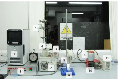
Figure 2.2.1. DFGF set up with electrical connections in red, separation channel fluid flow in

light blue and electrode channel fluid flow in dark blue. Supporting equipment: 1) Separation

channel buffer reservoir. 2) Computer controlled Flux Instruments Rheos2200 Pump. 3) 6 Port

switching valve. 4) Injection port. 5) DFGF device. 6) Outlet for sample collection. 7) Computer.

8) Computer controlled high voltage power supply. 9) Electrode channel buffer reservoir with

cooler. 10) Peristaltic pump. 11) De-gasser 12) Nikon D80 digital SLR camera with 60mm

macro lens.

1 2

4

3 5

6

7

8 11 10 9

12 1

2 4

3

5

6 7

8

9

10

(40)

22 Figure 2.2.2. Side view of the DFGF channel configuration. Consisting of; 1) Packed separation channel. 2) Separate purge channel housing the electrodes. 3) Cellulose Dialysis Membrane dividing the two channels. 4) Platinum electrodes.

2.2.1. DFGF Configuration

The DFGF was setup as shown above in figure 2.2.1. The DFGF cell itself is

composed of two acrylic layers which combine to form two channels divided by

strip of cellulose dialysis membrane, detailed in figure 2.2.2. This dual channel

arrangement eliminates pH changes and gas evolution from the separation channel

which can be detrimental to separation6_{. Cellulose dialysis membrane}7_{is used as it}

allows the EFG to propagate through into the separation channel by allowing small

ions to pass through. However large species, i.e. the sample, cannot permeate the

membrane, therefore are trapped in the separation channel preventing them from

being electrolysed. Gases and other electrolysis products are also unable to pass

through the membrane from the electrode channel. Constant flow of buffer through

electrode channel flushes away these species. The computer controlled Flux

Instruments Rheos 22008_{pump drives the hydrodynamic flow of buffer though the}

injection valve into the cell and on to collection or further detection. The peristaltic

pump circulates buffer solution around the electrode channel via a degasser to

remove any electrolysis gasses. 1

2

4

(41)

23

The dynamic electric field gradient is supplied and manipulated from the Protasis9

voltage array using Labview control software (appendix B). Detection is performed

by a Nikon D80 digital SLR camera with 60mm Macro lens10_.

Separations are monitored and controlled in real time using the computer and an

assortment of software. Before the DFGF is operated the separation channel must

be packed with a packing media to provide a narrower diffusion pathway through

the separation channel and to lower the solvent volume present. As the dimensions

of these channels are at the millimetre scale, any focusing would require an

extremely high voltage to apply an EFG capable of counteracting such a larger

volume without a packing material or monolith.

2.2.2. Packing Method

The DFGF was prepared for packing by rinsing components with deionised water.

Regenerated cellulose dialysis membrane with a molecular weight cut off (MWCO)

twice that of the intended analyte was cut to the dimensions 20mm wide and 90mm

in length. With the membrane in place on the Teflon gasket the two halves of the

DFGF cell are bolted together, tightening the bolts sequentially across opposite

corners. The separation and purge channels were then tested for leaks. A 1/16” in

line frit and 0.030" ID PEEK capillary tubing was connected to the outlet of the

separation channel. The same ID PEEK tubing was also connected to the inlet

having been connected to the packing reservoir and vibrating packing apparatus.

The cell was then immersed in the sonic bath and the reservoir charged with 500mg

of Bio-Rad 45-90µm spherical polyacrylamide11_{packing material suspended in}

(42)

24 Compressed air was used to charge the separation channel with the packing slurry.

Packing solvent was pushed through the channel for 3hours at a constant pressure

of 4bar. The system was then equilibrated for 24hours at 1µLmin-1_{with Flux}

Instruments Rheos 2200 pump8_{. The DFGF packing apparatus configuration is}

shown below, figure 2.2.3.

Figure 2.2.3. DFGF packing apparatus. 1) Compressed Air Supply with Pressure Gauge. 2) Slurry Reservoir. 3) Vibrating Motor. 4) DFGF Device. 5) Sonic Probe. 6) Beaker with DFGF submerged in water and sonic probe. 7) DFGF Outlet.

4

1

1 2

3 2

4

5 ₅

3

6

7

[image:42.595.109.525.241.578.2]

(43)

25 2.2.3. General Operation

In general the operation of the device would follow this standard procedure. A

linear EFG of around 80% of the maximum field, using ~800V across the length of

the separation channel, was applied for 20mins before each experiment to ensure

equilibration of the packed bed. The hydrodynamic flow of 50mM tris HCl buffer

solution was pumped through the separation channel at 1µLmin-1_{. Next the sample}

was loaded into the sample loop which was then switched in.

Once the sample was visible in the cell ~30mins was left for the sample to reach a

stable focal point. Typically, the linear EFG would be adjusted with the aim of

separation. If samples were separated the electric field was manipulated manually,

meaning overriding a linear gradient to produce bespoke voltage profiles, to hold a

single species back and allow the others to elute off the device. Alternatively, the

bands would be moved back down the column to refocus and increase the

separation by increasing the EFG. Additionally, the flow rate was altered to further

focus bands of sample giving dynamic flow as well as dynamic field. On injection

of the sample, images of the separation channel were collection at regular intervals

to record the separation. Each aspect of this control is explained in more detail

below.

2.2.4. Dynamic Flow Control: Flux Instruments Rheos Pumps and Janeiro 3.0

Incorporating the Flux Instruments Rheos 2200 pump8_{into the DFGF set up adds}

dynamic control over the flow rate used resulting in the technique being Dynamic

Flow Dynamic Field Gradient Focusing. These pumps are controlled over RS232

(44)

26 This computer control enables the flow rate to be adjusted in the order of

±0.1µLmin-1_{. Most piston pumps used in chromatographic techniques give a}

pulsing flow which worsens as the flow rate is lowered12_{. The Rheos 2200 pump}8

utilises a pulse dampening system to result in a stable flow even at flow rates as low

as 0.1µLmin-1_.

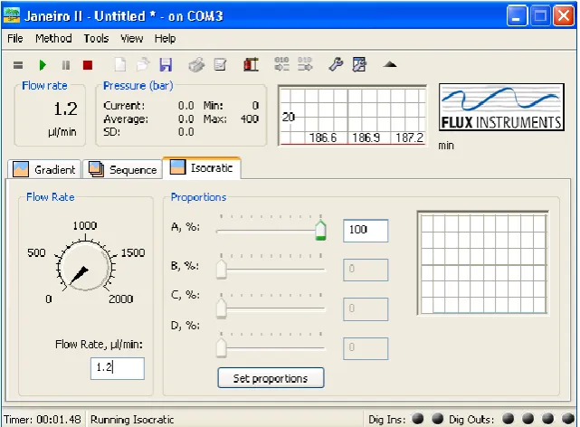
The Flux Instruments Janeiro control software allows control over a number of

parameters which are advantageous for DFGF. Figure 2.2.4 displays the user

interface of Janeiro. The flow rate can set by adjusting the dial controller or by

entering a value into the flow rate input. Also the maximum pressure and warning

pressure can be set to stop the pump in the event of a sudden increase in pressure

[image:44.595.159.480.392.628.2]

which could cause the packing or membrane to fail.

(45)

27 2.2.5. Dynamic Electric Field: Power Supply and Control

The supporting equipment for the Protasis device, figure 2.4.1, is the equipment

which has been used for all of the experimentation throughout this thesis. The

power supply consists of four individual UltraVolt High Voltage generators13

connected to respective high voltage (HV) outputs sharing a common ground rail

with a designated HV connection.

The HV generators were controlled independently by analogue signals from a

universal serial bus (USB) interface board, shown in figure 2.2.5.

(46)

[image:46.595.123.517.71.404.2]

28 Figure 2.2.6. Protasis UController HV Control Software. 1) Voltages supplied to electrodes. 2) Electrode Spacing. 3) Mode selector switch. 4) EFG Value. 5) Indicator Lights. 6) Electric field profile. 7) Power off button.

The Protasis DFGF Power Supply Unit was controlled by bespoke software

(appendix B) written in National Instruments LabView. The user interface, figure

2.2.6, enables control of the system in two modes, manual and automatic. Firstly, in

automatic mode, the software uses the value entered for electrode spacing to

calculate the maximum electric field gradient and uses this to calculate the required

voltage for each of the four positive electrodes to generate the gradient entered by

the user. In this mode the system designates the voltages applied to the electrodes

according to the linear EFG entered. 1

2

4

5 3

6

(47)

29 A linear EFG is where the slope of the gradient is the same between all of the

electrodes. An example of a linear EFG is shown in figure 2.2.7 with the

corresponding applied voltages and electrode spacing. The specified gradient is

plotted on a histogram shown in the bottom left of the interface, figure 2.2.6.

Figure 2.2.7. An example of a linear EFG generated by the Protasis Labview Ucontroller software in Automatic Mode. The dashed red line highlights the linear Electric Field Gradient.

In manual mode the software enables direct control of each electrode independently

using the sliders in the top left of the interface (figure 2.2.6), to apply different

gradients in different regions of the device, i.e. the EFG between each of the

electrodes can be different, figure 2.2.8. This level of control enables focused bands

(48)

30 Figure 2.2.8. An example of the EFGs which can be applied by the Labview Ucontroller software in Manual Mode. Notice the electric field gradient is no longer linear therefore the area on the bottom left is shaded out.

2.2.6. Data collection and presentation

A simple method of detection with DFGF was to use reflectance measurements

from digital exposures to monitor the position of bands in the separation channel.

Utilising a Nikon D80 DSLR camera10_{with a 60mm 1:2.8D macro lens, exposures}

were taken at set intervals incorporating the full length of the separation channel

(49)

31 Figure 2.2.9. A) Nikon D80 with a 60mm 1:2.8D macro lens configured to take images of the separation channel with the addition of a LED ring illuminator. B) Nikon Camera Control Pro software user interface.

By stacking these images in an image editing software, namely Adobe Photoshop or

GNU Image Manipulation Program (GIMP), it was possible to observe differences,

hence the position of a given analyte, by subtracting the first background image

from an image collected later. This preceding detection method is shown in figure

2.2.10A. For analysis of these subtracted images, “image analysis” software

ImageJ15_{was used to generate a ‘Profile Plot’ of the separation channel, shown in}

figure 2.2.10B.