One Dimensional Chemistry and the Generalised Local Density Approximation

(1)

One Dimensional Chemistry and the

Generalised Local Density Approximation

Caleb James Ball

February 2017

A thesis submitted for the degree of Doctor of Philosophy of The Australian

National University.

(2)

(3)

Declaration

The contents of this thesis have not been submitted for the award of any other degree

or diploma. Except where otherwise noted, the material is my own original work.

Caleb James Ball

20 February, 2017

(4)

(5)

Acknowledgements

Writing a Ph.D. thesis leaves one with many people to thank. Here are a few most

important to me:

Thanks Peter. After supervising my honours thesis you were brave enough to

take me on for a Ph.D. project. You’ve taught me a great deal about many different

things, but most of all I thank you for the immense wisdom you’ve shared over the

past years. I hope that when I look for a bug in some code in the future I will

remember all the times you told me to go back to the simplest case.

Thanks Titou. You’ve spent so much time with me that I consider your supervision

on equal footing with Peter’s. Many thanks for taking that burden on. I know I

caused you a lot of angst at various times, and I’m grateful that you kept putting up

with me. Hopefully we can share another beer sometime in the future, because at

the end of the day I’m going to miss your company.

Thanks Mum and Dad. I wouldn’t be here without you, in more ways than one!

You’ve given me more support than I could have asked for and it’s opened up so

many opportunities for me. I’m sorry I chose not to go to music school, hopefully

this makes up for it!

Thanks Fiorella. Thanks for sticking with me through thick and thin. You were

always there to cheer me up when I felt like things were looking pretty bleak, which

probably helped a lot more than I thought. I promise I’ll make our next adventure a

little smoother.

And thanks to everyone else. Thanks to the other members of the Gill group,

particularly Andrew, Giuseppe, Marat and Simon. Thanks to all my friends who’ve

watched as it all happened. Life would have been a lot duller had you not all been

there to brighten things up!

And thanks to the institutions who provided me funding: the Australian

Govern-ment and the ANU Research School of Chemistry for their scholarships as well as

the National Computing Infrastructure for their grants of supercomputer time.

(6)

(7)

Abstract

In this thesis we explore two distinct topics: a unique model of one dimensional

chemistry and the development of the generalised local density approximation.

The specific one dimensional system we study is one in which three dimensional

particles, both electrons and nuclei, have been strictly confined to move on a line.

This means we retain the Coulomb interaction of the three dimensional particles.

This is problematic, the singularity of this interaction is exceptionally strong in one

dimension and requires special techniques be used to circumvent it.

In our study we employ the Dirichlet boundary conditions, which require the

wavefunction to vanish whenever two particles touch. This brings some severe

consequences including, most controversially, that the nuclei are impenetrable to the

electrons. However it does permit finite binding energies of electrons to nuclei and

has a number of unique features which make it an interesting system to study for

insight into electron behaviour.

Here we explore the mechanics of chemistry within this model. We construct an

unusual periodic table for one dimensional elements and explore the mechanisms by

which they bind into molecules. Ultimately, we are able to develop a set of simple

rules with which one can easily predict the outcome of a reaction in this unique

model.

The generalised local density approximation is a new method for constructing

density functional approximations. The local density approximation, the most

simplistic of all density functionals, is built off the properties of the infinite uniform

electron gas and as result replicates them exactly. It is also possible to construct

finite uniform electron gases and, contrary to expectations, the regular local density

approximation is unable to model these finite gases correctly.

The generalised local density approximation incorporates these finite gases into its

construction. We account for their differences from the infinite gases by introducing

a new parameter which measures the proximity of electrons at a point in space.

We can then construct a correlation functional for one dimensional systems using a

method which closely resembles that used for previous local density approximations.

(8)

Because of the definition of the new parameter, one would formally consider this

functional to be a meta-GGA functional. However it retains the exceptionally simple

form of a local density approximation.

This new functional is observed to have greatly improved accuracy compared to

the standard local density approximation when tested against a variety of systems,

including reactions of the one dimensional molecules identified earlier. Although we

only construct a one dimensional functional here, the method is easily generalised to

(9)

List of Publications

The following papers have been published during the preparation of this thesis, and

their content appears within:

1. P. F. Loos, C. J. Ball and P. M. W. Gill, “Uniform electron gases. II. The

generalized local density approximation in one dimension”, J. Chem. Phys.

140, 18A524 (2014).

2. P. F. Loos, C. J. Ball and P. M. W. Gill, “Chemistry in one dimension”,Phys.

Chem. Chem. Phys. 17, 3196 (2015).

3. C. J. Ball and P. M. W. Gill, “Chem1D: a software package for electronic

structure calculations on one-dimensional systems”, Mol. Phys. 113, 1843

(2015).

4. C. J. Ball, P. F. Loos and P. M. W. Gill, “Molecular electronic structure in

one-dimensional Coulomb systems”, Phys. Chem. Chem. Phys. 19, 3987

(2015).

The following paper has also been published during the preparation of this thesis,

but does not appear within:

5. F. J. M. Rogers, C. J. Ball and P. F. Loos, “Symmetry-broken local-density

approximation for one-dimensional systems”,Phys. Rev. B 97, 235114 (2016).

(14)

(15)

Chapter 1

Introduction

1.1 Quantum chemistry

With the advent of quantum mechanics in the early twentieth century chemists

gained the necessary physical and mathematical tools to predict the outcome of many

chemical processes from first principles. The computational demands of this problem

are so immense that it has taken considerable time for this to become an attractive

exercise. The advances in both technology and theoretical understanding that have

occurred since have lead to this becoming a significant feature of the modern study

of chemistry.

Unfortunately, many chemical systems remain well outside the reach of modern

theoretical methods. And so extensive research still continues into the improvement

of these methods. In this thesis we will explore two main topics which relate to such

developments.

Our first topic concerns a newly defined model chemistry. Within this model are

some unique features that may allow for new insights into the behaviour of particles

in chemical systems. The second topic involves the initial development of a method

which builds upon one of the oldest and simplest. This construction takes a new

direction from the work preceding it which may also offer new insights and act as a

new base for further development.

Before we discuss these topics we will present some of the necessary background

to their discussion.

1.1.1 The Schr¨odinger wave equation

Within the field of quantum chemistry Schr¨odinger’s wave equation [1, 2] is the

dominant formulation of quantum mechanics. For our purposes we need only consider

(16)

the time-independent equation, which can be given as

ˆ

HΨ =EΨ (1.1)

where we have adopted atomic units, which will be used throughout this thesis unless

otherwise stated. This simple equation hides a wealth of complexity. In order to

observe this let us examine what the components of the equation are.

The Hamiltonian operator, ˆH, describes the energetic components of the system.

Most importantly it contains terms which describe the kinetic and potential energies

of a particle in the system being considered. In a complete treatment of a quantum

system it is not limited to this, and may, for example, contain terms which describe

the interaction of the particles with an external field. Such quantities will play only

a small role throughout the remainder of this thesis. Removing them leaves us with

the following Hamiltonian

ˆ

H= ˆTe+ ˆTN + ˆVee+ ˆVeN+ ˆVN N (1.2)

ˆ

Te and ˆTN are operators which describe the kinetic energies of the electrons and

nuclei respectively, while ˆVee, ˆVeN and ˆVN N describe the potential energy from the

interaction between electrons, electrons and nuclei and between nuclei.

The other key component of the Schr¨odinger wave equation is Ψ, the wavefunction.

This is a high dimensional function which completely describes the quantum state of

all the particles present within the system. In principle, with the knowledge of this

object it is possible to determine any physical property of the system.

Finally, theE in the wave equation is simply the total energy of the system, a

scalar quantity. Hence the equation describes what is known as aneigenproblem. We

begin with knowledge of ˆH, which can be constructed for a given system of particles.

From this we search for a function Ψ which when acted upon by ˆHwill be unchanged

apart from a constant factor.

Unfortunately, despite such problems being widely studied by both

mathemati-cians and physicists, the Schr¨odinger wave equation is unable to be solved analytically

(except in a handful of special cases). This should not be surprising; the potential

interactions couple the movement of particles together, resulting in this being

equiv-alent to the many-body problem of classical physics. A solution to that problem has

thus far eluded physicists for centuries, so we are reduced to finding approximations

to the solution of the equation. Before we explore some of these approximations, we

(17)

1.1. QUANTUM CHEMISTRY 3

1.1.2 The Pauli exclusion principle

As stated above, the wavefunction is a complicated object which describes the

quantum state of the particles in a system. An important principle of quantum

mechanics is that two electrons (or more generally, two fermions) cannot occupy the

same state. This is called the Pauli exclusion principle, after the physicist who first

described it [3].

This has an important manifestation in the mathematics of the Schr¨odinger wave

equation. It requires that the wavefunction be antisymmetric with respect to the

exchange of any two electrons. That is to say

Ψ(. . . ,xi,xj, . . .) =−Ψ(. . . ,xj,xi, . . .) (1.3)

where xi and xj are the full coordinates of two electrons, including both their

positional vectors (ri and rj) and their spin coordinates (si and sj).

Spin is a quantum mechanical property of an electron, and represents a type of

momentum intrinsic to a particle. In the case of electrons it can take one of two

values, either +1/2 or−1/2. This spin coordinate is part of the quantum state of an

electron (the remainder being its spatial description), and a chemically important

consequence of this principle is that any spatial quantum state can be occupied by

up to two electrons, and no more, at any one time.

1.1.3 Observables and self-adjoint operators

From the wavefunction one can findany observable quantity of the system. One of the

tenets of quantum mechanics is that an observable quantity can be described by what

is called a self-adjoint operator. An operator ˆO is self adjoint if hf,Oˆgi=hOˆf, gi. In the Hilbert space used in quantum chemistry this statement becomes

Z

f∗(r) ˆOg(r)dr=

Z

g∗(r) ˆOf(r)dr (1.4)

hf|O|ˆ gi=hg|O|ˆ fi (1.5)

where hf|O|ˆgiis the Dirac notation that is common in the study of quantum physics.

A simple example of this is determining the energy of a wavefunction. In this

case the Hamiltonian itself is the self-adjoint operator, and the energy is given by

E =hΨ|Hˆ|Ψi=

Z

Ψ∗(x) ˆHΨ(x)dx (1.6)

(18)

Later, it will be important to note that the relationship between observable

quantities and self-adjoint operators is an equivalence. Hence we can state that if an

operator isnot self-adjoint then it cannot describe an observable quantity.

1.1.4 The variational principle

Eigenproblems such as the Schr¨odinger wave equation permit a spectrum of

solu-tions. For simplicity’s sake, we’ll assume that the spectrum is discrete rather than

continuous. One of the solutions, which we label Ψ0, must then have the lowest

energy. Enumerating the other solutions as Ψi, the corresponding eigenvalues Ei

satisfyE0< Ei for all i6= 0.

This solution is called the ground state, and is the state that the system will

prefer to occupy. The variational principle states that any approximate, or trial,

wavefunction must then be higher in energy, that is

E0≤ hΨtrial|Hˆ|Ψtriali (1.7)

where Ψtrial is the approximate wavefunction, which we assume here to be normalised.

This results in the true energy being a lower bound to the energy of any approximation

to the true wavefunction.

This is an incredibly useful result, as it allows us to judge the relative quality of

different approximate wavefunctions. Not all quantum chemistry methods use the

variational method to obtain their estimate however, but we will discuss one which

does shortly.

1.1.5 The Born-Oppenheimer approximation

The complete Schr¨odinger wave equation treats all particles within a system in an

identical manner. In any given molecule we consider two kinds of particles: electrons

and nuclei. There is an enormous disparity in the mass of these two particles however;

nuclei are much more massive than electrons. As a consequence of this electrons

have far greater kinetic energy than the nuclei.

This observation leads to a first, and very common, approximation that was

originally described by Born and Oppenheimer [4]. From the perspective of the

electrons, the nuclei move so slow that they are essentially stationary. More rigorously,

(19)

1.2. THE HARTREE-FOCK METHOD 5

operator where the nuclei are fixed in place

ˆ

Helec = ˆTe+ ˆVee+ ˆVeN (1.8)

ˆ

HelecΨelec =EelecΨelec (1.9)

The result of this equation is anelectronic wavefunction which describes only the state

of the electrons. This is thenparametrically dependent upon the nuclear coordinates;

for every possible arrangement of the nuclei there is a unique electronic wavefunction.

The total energy can then be obtained by simply adding the energy originating from

the Coulombic repulsion between the nuclei to the electronic energy.

Having solved the electronic problem it is then possible to construct the total

wavefunction by factoring in the motion of the nuclei. If we continue the same line

of reasoning then we can approximate the effect of the electrons on the nuclei by

considering only their average field.

Although not always the case, this assumption typically yields extremely accurate

approximations. For the remainder of this thesis we will take the Born-Oppenheimer

approximation as given, and will concern ourselves only with the determination of the

electronic wavefunction. As such we will no longer explicitly refer to the electronic

wavefunction, shortening this to just “the wavefunction”. Any reference to the energy

of a molecule will refer to the total energy, i.e. the sum of the electronic energy and

the nuclear repulsion, unless otherwise stated.

1.2 The Hartree-Fock method

1.2.1 The Hartree-Fock wavefunction

Although the Born-Oppenheimer approximation significantly simplifies the wave

equation the electronic wavefunction is still a much too complicated object to, at

least in general, find analytically. This difficulty is caused by the coupling of electron

motion via the Coulomb operator. If we were to decouple the electrons, however, the

problem would be reduced to one that could be much more easily solved.

To achieve this decoupling we begin by introducing an ansatz wavefunction. This

was a key suggestion by Hartree [5], who proposed approximating the wavefunction

with the following form

ΨHartree(x1,x2, . . . ,xN) = N

Y

i=1

(20)

where the functions ψi are referred to as molecular spin orbitals. These are

wavefunction-like objects that describe the quantum state of a single electron, rather

than the whole ensemble. Note that each spin orbital is a product of a spatial

orbital ψi(ri), which describes the movement of an electron through space, and a

spin function that encodes the spin state associated with the orbital.

Such a wavefunction does not satisfy the antisymmetry requirement that Pauli’s

exclusion principle demands. This was independently observed by both Fock [6]

and Slater [7] shortly after Hartree’s initial proposal. Slater suggested correcting

the problem by expanding the simple product into a determinant which correctly

captures the required antisymmetry.

ΨHF(x1,x2, . . . ,xN) =

ψ1(r1, s1) ψ1(r2, s2) · · ·

ψ2(r1, s1) ψ2(r2, s2) · · ·

..

. ... . ..

(1.11)

A determinant of this kind is referred to as a Slater determinant. By invoking

the variational principle and minimising the total energy of this determinant we

obtain a useful approximate wavefunction. This wavefunction is referred to as the

Hartree-Fock wavefunction and the method through which it is constructed the

Hartree-Fock method (often simply shortened to Hartree-Fock and abbreviated as

HF).

In this section we will give an overview of some of the details of this method,

and is largely based upon the truly comprehensive description in the classic text by

Szabo & Ostlund[8]. However in the following chapters spin will have a vanishing

role in the mechanics of the calculations, and so from here on we will omit the details

of its involvement in computation, preferring to work with the spatial orbitalsψi(ri)

where possible.

1.2.2 The Fock potential

The variational theorem tells us that to find the correct Hartree-Fock wavefunction

we must obtain the Slater determinant with the lowest possible total energy. To

(21)

from the set of orbitals{ψa, ψb, ψc. . .}is given by the expression

E=hΨHF|Hˆ|ΨHFi (1.12)

=X

a

ha|ˆh(1)|ai+1 2

X

ab

(aa|bb)−(ab|ab) (1.13)

=X

a

ha|ˆh(1)|ai+1 2

X

ab

(aa||bb) (1.14)

ˆ

h(1) =−1

2∇ 2 1+ X A ZA

r1A

(1.15)

where ZAis the charge of nucleus A andr1A is the distance between electron 1 and

nucleus A. We have used chemist’s notation for the two electron integrals (aa|bb),

the use of which will continue throughout this thesis.

If we constrain the orbitals such that they are orthonormal to each other,

hψi|ψji=

Z

ψi(r)∗ψj(r)dr=δi,j (1.16)

where δi,j is the Kronecker delta function, then through a derivation of significant

length we find that the correct HF orbitals are those which solve the equation

"

ˆ

h(1) +X

b

J_b(1)−X

b

K_b(1)

#

ψa(1) =εaψa(1) (1.17)

where we have introduced the three new operators ˆh(1), J_b(1) and K_b(1). The

one particle operator ˆh(1) collects the kinetic energies and the potential energies

generated by the interaction between the nuclei and electrons, which are unchanged

from the regular Schr¨odinger equation.

The other two operators J_b(1) and K_b(1), which are both two particle operators,

do not appear in the Schr¨odinger equation. These operators are mean-field

approxi-mations to the correct electron-electron potential operator. That is, they give the

potential interaction of an electron with the averaged field of the other electrons.

J_b(1) gives the classical Coulomb interaction between two charged particles, while

K_b(1) returns the so called exchange interaction of quantum mechanical systems,

which arises as a consequence of the antisymmetry of the wavefunction. These

expressions can be defined as

Jb(1)ψa(1) =

Z _|

ψb(2)|2

r12

dr2ψa(1) (1.18)

K_b(1)ψa(1) =

Z _ψ

b(2)∗ψa(2)

r12

(22)

The key gain of this process is that the overall operator is identical for every

electron in the system. This allows us to define a one electron operator called the

Fock operator,

ˆ

f(1) = ˆh(1) +X

b

J_b(1)− K_b(1), (1.20)

and write the HF equations, those which give the orbitals that construct the lowest

energy single Slater determinant, as

ˆ

f ψa=εaψa. (1.21)

Note that the Fock operator is dependent upon the orbitals ψa, resulting in this

equation becoming a non-linear eigenfunction problem. While solving this problem

and obtaining the correct HF solution is possible in principle, it is ill-suited to large

scale attack by computer. Given the size of most molecular systems this quickly

becomes necessary.

1.2.3 The Roothaan-Hall equations

The Fock potential allows us to approximate the complicated Schr¨odinger wave

equation by a system of much simpler equations. This does not, however, permit

a useful, generally applicable algorithm to obtain the solution. To achieve this we

will introduce the Roothaan-Hall [9, 10] equations which, by introducing a basis set

for expanding the orbitals, reduces the problem to an iteratively solvable matrix

equation.

More specifically, we will introduce a slight variation of the Roothaan-Hall

equations. This method was first described for closed-shell systems, i.e. where all

the spatial orbitals are doubly occupied by a spin-up and a spin-down electron. Here

we will describe the equations for a fully ferromagnetic system, i.e. where all the

spatial orbitals are occupied by a single spin-up electron.

Strictly speaking, this is a different special case of the Pople-Nesbet equations,

which generalise the Roothaan-Hall equations to any open-shell system [11]. Later

in this thesis we will be considering ferromagnetic systems exclusively, and so a full

description of the Pople-Nesbet equations will not be required.

The first step in this process is introducing a basis set for describing the spatial

(23)

expand the orbitals as a linear combination

ψa= M

X

µ=1

ca,µφµ (1.22)

This is only exact if the chosen basis set is complete over the space in which the

functionψa resides. In this case, such a requirement usually demands that the basis

set be of infinite size. This is not possible from a computational perspective, and so

finite basis sets are used and the expansion in Eq. (1.22) is only an approximation.

The closer the basis set is to completeness, the better this approximation becomes.

There are many possible choices of basis set, and later in this thesis such choices

will be discussed. For the remainder of this section the precise nature of the basis

set is unimportant and so we will not concern ourselves with these details.

If we substitute the Eq. (1.22) into the HF equation obtained above, Eq. (1.21),

it can be reduced to a matrix equation by introducing the four matrices

Ci,j =ci,j (1.23)

εi,j =δi,jεi (1.24)

Sµ,ν =

Z

φ∗_µφνdr (1.25)

Fµ,ν =

Z

φ∗_µf φˆ νdr (1.26)

like so

FC=εSC. (1.27)

The matrices Cand εnow contain the coefficients in the expansion of Eq. (1.22)

and the energies of the molecular orbitals. Scontains the overlap between the basis

functions used and is, unsurprisingly, called the overlap matrix. We can also define a

charge density matrixP

Pµ,ν =

X

a

Cµ,aC∗ν,a. (1.28)

which simplifies the definition of the matrix F, typically called the Fock matrix, as

follows

Fµ,ν =

Z

φ∗_µhˆ(1)φνdr+

X

λσ

Pλσ

(µν|λσ)−(µλ|νσ)

=

Z

φ∗_µhˆ(1)φνdr+

X

λσ

(24)

It is important to observe that for an orthonormal basis the overlap matrix would

simply be the identity matrix, since by the definition of orthonormal functions (in

the spaceL2) we find

Z

φ∗_µφνdr=δi,j. (1.30)

While it is common to employ a normalised basis set it is rare for it to also be

orthonormal, at least for computations on molecular systems. This makes it necessary

to introduce an orthogonalisation procedure which involves diagonalising the overlap

matrixS. This can be problematic if there is near linear dependence in the basis set,

as it can lead to numerical instabilities.

The result of the orthogonalisation is a transformation matrix, usually calledX,

which moves between the chosen basis set to an orthogonalised set. This allows us to

recast Eq. (1.27) as a simple matrix eigenproblem

F0C0 =εC0 (1.31)

where the primes indicate the matrices have been transformed into the orthogonal

basis. If we can construct the Fock matrixF, then diagonalising F0 allows us to

generate both εand C0. We need only apply the transformationX to return the

coefficient matrix back to the original basis to obtain the solutionC.

Unfortunately, the dependence of the Fock matrix F on the coefficient matrix

C (via the density matrix P in Eq. (1.29)) causes this to remain a non-linear

eigenproblem. While this makes a direct solution difficult, an iterative scheme can

be used to solve the problem.

The equivalence in Eq. (1.27) only holds for the correct coefficient matrix C.

That is, if we generate the Fock matrixF fromCthis relationship is only true ifC

is the correct solution. In an iterative scheme we begin with a trial set of coefficients

C0 that we use to generate a Fock matrix. We can then follow the procedure to

obtain a new coefficient matrixC1.

Should C1 ≈C0, using some chosen metric and to within some threshold, then

we know thatC0 solves the equations. In the more likely case that it is not, then

we can construct a new Fock matrix from C1 and repeat the process. Ideally, if we

continue this process then we will eventually converge to a solution. This method is

called the self consistent field (SCF) method, since we search for a solution which is

consistent with the field that it generates.

There is no guarantee of convergence during this process, and both the success of

the process and the speed with which the solution is found depend heavily upon the

(25)

1.3. WAVEFUNCTION-BASED CORRELATED METHODS 11

is not necessarily a trivial process. Additionally, there are multiple techniques for

improving the convergence behaviour which can be added to the algorithm (perhaps

most notably the DIIS method of Pulay [12, 13]). Fortunately, in this thesis we

will not find ourselves grappling with such difficulties, and so we will omit further

discussion of this topic.

1.2.4 Aftermath

With the Roothaan-Hall equations constructed, we now have a general method for

solving an approximation to the Schr¨odinger wave equation. The question remains:

is this approximation any good? As it turns out, the Hartree-Fock wavefunction

yields an excellent approximation to the total energy of a molecular system.

It is unfortunate that quantum chemists are rarely interested in the raw total

energies of molecules. It is differences that are typically required when asking chemical

questions. At the simplest level, a reaction being favourable depends upon whether

the products of a reaction have a lower energy than the reactants. Similarly, when

considering the kinetics of a reaction it is the height of the transition barrier that is

essential, which is the difference between the energy of the transition state and the

reactants.

During most reactions the vast majority of a molecule’s total energy is unchanged.

The nuclei still attract the electrons by a similar amount, and the electrons,

par-ticularly those close to the nuclei, maintain a similar level of kinetic energy. The

consequence is that the small fraction of the total energy missed by the Hartree-Fock

approximation is essential to describing the energetics involved in chemistry.

1.3 Wavefunction-based correlated methods

The difference between the Hartree-Fock energy and the exact energy is called the

correlation energy,

Ec=E−EHF. (1.32)

Because the Hartree-Fock energy is a variationally minimised approximation to the

exact energy it must be greater than the exact energy. As a result the correlation

energy is a negative number, and represents stabilising forces which are not accounted

for in the Hartree-Fock method and wavefunction.

This difference is a consequence of the Hartree-Fock potential being a

mean-field approximation: each electron feels the averaged electric mean-field generated by the

(26)

positions of each other they would be capable of relaxing into more energetically

favourable orbits by correlating their movement with one another. This is the source

of both the correlation energy’s physical nature and the name given to it.

In this section we will describe a collection of methods for estimating the

correla-tion energy of a molecule that will be used later in this thesis. For the moment we

will restrict ourselves to wavefunction-based methods, i.e. those which primarily work

with the wavefunction to obtain their estimate. There is another class of correlated

methods which are based on the electron density that we will discuss afterwards.

1.3.1 Møller-Plesset perturbation theory

A powerful and well established method for finding an approximate solution to

a difficult problem is perturbation theory. The idea is to find an exact solution

to a simplified version of the problem that needs to be solved. This is also an

approximation to the solution of the original problem, and the closer the simplified

problem is to the original, the better the approximation.

The difference between the original and the simplified problem can then be seen

as a perturbation to the simplified problem. Perturbation theory observes how this

difference affects the approximate solution and from this attempts to correct the

approximation. The standard perturbation technique used in quantum chemistry

is Møller-Plesset theory [14], which is an application of Rayleigh-Schr¨odinger (RS)

perturbation theory [2, 15] to the correlation problem.

RS perturbation theory separates the Schr¨odinger equation in the following

manner

ˆ

HΨ = ˆH0Ψ +λVˆΨ =EΨ (1.33)

where the operator ˆH0 is chosen such that the solution to the equation

ˆ

H0Ψ(0)=E(0)Ψ(0) (1.34)

is known.

To obtain a solution to this problem both the wavefunction and energy are

expanded as a power series inλ

Ψ = Ψ(0)+λΨ(1)+λ2Ψ(2)+. . . (1.35)

E =E(0)+λE(1)+λ2E(2)+. . . (1.36)

This expansion can be substituted into Eq. (1.33) and the coefficients of the powers

(27)

and E(0) to the unknown terms of Eqs. (1.35) and (1.36). Ultimately, this allows us

to express the terms of the energy expansion using the spectrum of ˆH0.

It was Møller and Plesset who first described the application of RS perturbation

theory to molecular systems [14]. Their formulation uses the Hartree-Fock

wave-function as the starting point for the perturbation, i.e. ˆH0 is taken to be the Fock

operator. This leaves the perturbation operator ˆV as the difference between the

exact Coulomb potential and the mean-field approximation of the Fock potential

ˆ

V =X

ij

r−_ij1−X

b

J_b(1)− K_b(1) (1.37)

where both Jb(1) andKb(1) have been defined in Eqs. 1.18 and 1.19 respectively.

Having made this separation the terms of Eq. (1.36) can be cast in terms of

integrals over the HF molecular orbitals. These quickly become lengthy (but not

necessarily complicated), however the first few are given by the relatively simple

expressions

E0 =

X

a

a (1.38)

E1 =−

1 2

occ

X

ab

(aa||bb) (1.39)

E2 =

1 4

occ

X

ab

virt

X

rs

|(ar||bs)|2

a+b−r−s

(1.40)

where ψa and ψb represent occupied HF orbitals and ψr and ψs are unoccupied

(virtual) HF orbitals. Partial summations of this series give approximations to the

true energy of the system. The energy of the HF wavefunction is given by the sum

of the zero-th and first order term (EHF=E0+E1), so the first correlated energy

estimate is given by the second-order sum. This approximation is referred to as MP2,

and including higher terms gives the MP3 energy, MP4 energy and so on.

In principle the infinite summationP

nEn gives the exact energy. Unfortunately,

for many molecular systems, this summation begins diverging shortly into the

sequence of partial sums[16]. Furthermore, higher order corrections quickly escalate

in computational difficulty. For these reasons only the low order corrections are

commonly used (i.e. MP2, MP3 and occasionally MP4).

1.3.2 Configuration interaction

While Møller-Plesset theory is a useful method for obtaining low cost corrections

(28)

accuracy. Configuration interaction (CI) is another method, even simpler in concept,

for obtaining a correlation energy [8]. The key draw for the CI method is that, when

used to its full extent, it is capable of finding the exact solution to the Schr¨odinger

equation.

Where the HF wavefunction is a Slater determinant constructed from a set of

one-electron spin orbitals, the CI wavefunction builds upon HF by using a linear

combination of Slater determinants. The set of determinants used for the CI

wave-function is composed of all the determinants Ψi that can be constructed by occupying

different configurations of the HF orbitals.

The final CI wavefunction is found by choosing the coefficients in the linear

expansion which, according to the variational theory, minimise the total energy. This

is achieved by constructing a Hamiltonian matrix which describes the interactions

between the determinants, and has the elements

Hij =hΨi|Hˆ|Ψji. (1.41)

The lowest eigenvalue of this matrix is the exact ground state energy of the system,

within the limits of the basis set employed during the initial HF calculation. The

cor-responding eigenvector contains the coefficients of the determinants in the expansion

of the ground state wavefunction.

The method described above is referred to as full CI since it makes use of the

full set of determinants. Although this method gives the correct answer to the

Schr¨odinger equation (when used within a complete basis set) it is rarely used due

to its computational expense. Constructing the determinants is a combinatorial

problem, and leads to a factorial scaling with system size. For all but the smallest

and simplest of systems this problem is intractable.

It is, however, possible to truncate the set of determinants used in the

wavefunc-tion expansion. For example, in the CISD method only those determinants which

differ from the ground state determinant by one (single excitations) or two (double

excitations) orbitals are included in the basis set. This makes a significant difference

to the computational scaling of the method by dramatically reducing the number

of possible determinants. However, it does introduce its own difficulties. In this

thesis we will employ the CI method in order to generate high accuracy reference

values for systems where the Full CI problem is tractable, and so we will refrain from

(29)

1.3.3 Quantum Monte Carlo

Quantum Monte Carlo (QMC) is a stochastic numerical method. It differs from the

previously described correlated methods by not being a strictly post HF correction.

In QMC, the energy of an ansatz wavefunction is directly evaluated via numerical

methods and the wavefunction manipulated to achieve the best possible energy. Like

Full CI, QMC is capable of obtaining the exact energy and wavefunction in principle.

Depending on the required precision, however, it may become intractable to do so,

and the method has other limitations which may prevent it from achieving the correct

solution.

A QMC calculation typically employs two separate steps. A Variational Monte

Carlo (VMC) step generates a high accuracy first approximation to the solution.

This result is then fed to a Diffusion Monte Carlo (DMC) step, which relaxes the

wavefunction further and is capable of extremely high accuracy at the cost of slowly

converging results. This theory only makes a brief appearance later in this thesis,

and so we will refrain from exploring the details of the construction.

In VMC a trial wavefunction ΨT(q;r) is chosen with a set of variable parametersq.

The variational principle is invoked and these parameters are optimised to minimise

the energy of the wavefunction. The key feature of VMC is that the energy is found

by directly evaluating the integral

E= hΨT| ˆ H|ΨTi

hΨT|ΨTi

=

R

|ΨT(q;r)|2ELdr

R

|ΨT(q;r)|2dr

(1.42)

where

EL=

ˆ

HΨT(q;r)

ΨT(q;r)

(1.43)

is known as the local energy. This is done by using an importance sampling of the

distribution|ΨT(q;r)|2.

Unlike what has been discussed previously, DMC makes use of the time-dependent

Schr¨odinger wave equation. Again, a trial wavefunction is used, and it is allowed

to propagate through imaginary time. One can show that through this process the

wavefunction will eventually reach the exact ground-state solution. The

propaga-tion step requires a high-dimensional integral involving the wavefuncpropaga-tion, which is

(30)

1.4 Density Functional Theory

For most of the twentieth century wavefunction based methods were the prevailing

approach for solving the Schr¨odinger equation for chemical systems. It is not the

only way to approach the problem however. Modern computational chemistry is

dominated by Density Functional Theory (DFT), a very different approach to working

with the Schr¨odinger equation.

Rather than focussing on describing the wavefunction, DFT methods work with

the electronic density instead. This was shown to be possible by Hohenberg and

Kohn in their seminal 1964 paper [17], in which they prove that the ground-state

properties of a system are uniquely determined by the electronic density. Modern

applications of this theory also rely upon the Kohn-Sham equations [18], which

provide a similar framework for DFT as HF theory does for wavefunction methods.

1.4.1 The Hohenberg-Kohn theorems

The validity of DFT rests upon two proofs given by Hohenberg and Kohn [17]. In

order to explore these theorems let us define a Hamiltonian

ˆ

H= ˆT+ ˆU + ˆV (1.44)

ˆ T =−1

2

X

i

∇2_i; Uˆ =X

i,j

1

|ri−rj|

; Vˆ =X

i

ν(ri) (1.45)

whereν(r) is an external potential in which the electrons are moving. In a molecular

system this potential would be the one generated by the nuclei. We will also assume

that this Hamiltonian permits a non-degenerate ground-state wavefunction Ψ, with

an associated electronic densityρ that is given by

ρ(r) =

Z

|Ψ(r, s1,x2,x3, . . .)|2ds1dx2dx3. . . dxN (1.46)

The first Hohenberg-Kohn theorem proves that a given electronic density uniquely

determines the external potential. To prove this let a second potentialν0(r) define

a Hamiltonian ˆH0. This Hamiltonian has an associated wavefunction Ψ0 that we

will assume generates the same density, ρ, as the first wavefunction Ψ. We know

(31)

1.4. DENSITY FUNCTIONAL THEORY 17

principle we find

E0 =hΨ0|Hˆ0|Ψ0i

<hΨ|Hˆ0|Ψi

<hΨ|Hˆ −Vˆ + ˆV0|Ψi

< E+hΨ|Vˆ0−Vˆ|Ψi (1.47)

and similarly

E < E0+hΨ|Vˆ −Vˆ0|Ψi (1.48)

Summing equations (1.47) and (1.48) gives the contradiction

E+E0< E+E0 (1.49)

proving that no two external potentials can generate the same electronic density.

The key consequence of this theorem is that there is no information lost by

ignoring the wavefunction in favour of the density. This implies it is possible to

extract any observable property of a quantum system from its density. A simple

example of this would be a functional Eν[ρ] which extracts the energy of a density ρ

in the potential field of ν.

The second of Hohenberg and Kohn’s theorems concerns such a functional,

asserting that it is minimised by the density which corresponds to the given external

potential. This is an extension of the variational principle of the wavefunction to the

electronic density.

To prove this we define a Hamiltonian ˆH with an external potential ν. This

permits a wavefunction Ψ with an associated density ρ which we will compare

with a trial density ρ0. From the first theorem we know that this trial density

uniquely determines an external potentialν0, which in turn defines a Hamiltonian

for which a wavefunction Ψ0 can be found. By applying the variational theorem to

this wavefunction it follows that

Eν[ρ0] =hΨ0|Hˆ|Ψ0i ≥Eν[ρ] =hΨ|Hˆ|Ψi (1.50)

While the Hohenberg-Kohn theorems provide an alternative route to approach

the Schr¨odinger wave equation there is a significant barrier to its use. The theorems

are non-constructive in nature, and so while we know an exact energy functional

exists, we do not know what it is. Unfortunately deriving such a functional turns

(32)

Of particular note is the difficulty in deriving a functional which correctly evaluates

the kinetic energy, a quantity which would be considered trivial in wavefunction

based methods. This problem is neatly sidestepped by working in the Kohn-Sham

formalism, which introduces aspects of wavefunction theories in order to simplify the

problem of optimising the electronic density.

1.4.2 The Kohn-Sham equations

The Kohn-Sham (KS) equations form the basis for the application of DFT in

modern chemistry by providing a framework for optimising the electronic density

self-consistently [18]. This is achieved by defining a set of non-interacting electron

orbitals that have the same electronic density that generates the external potential

of the desired system. The result bears a great deal of similarity to the approach

of Hartree-Fock theory. It does, however, provide facility for the introduction of

correlation effects by means of an appropriate density functional.

From the Hohenberg-Kohn theorems we know that the ground state energy of a

Hamiltonian defined by the external potentialν can be written as

E0 =

Z

ρ(r)ν(r)dr+1 2

Z Z

ρ(r1)ρ(r2)

r12

dr1dr2+T[ρ] +F[ρ] (1.51)

whereρ is the ground state electronic density that produces the potentialν. The

first and second term give the interaction of the electrons with the external potential

and the mean-field Coulomb interaction respectively. The functionalT[ρ] gives the

kinetic energy of the electrons while F[ρ] describes the exchange and correlation

effects.

We also know that this energy is minimised byρ, and so we can determine via

calculus of variations that

Z

δρ(r)

νeff(r) +

δT[ρ]

δρ +νxc[ρ(r)]

dr= 0 (1.52)

where we have defined

νeff(r) =ν(r) +

Z

ρ(r0)

|r−r0_|dr 0

(1.53)

νxc(ρ) =

δF[ρ]

δρ (1.54)

Kohn and Sham observe that this same expression is obtained by applying the

Hohenberg-Kohn theorems to a system of non-interacting particles that move within

(33)

obtain the density of the interacting system from the orbitals obtained by solving

the one-particle equations

−1

2∇

2₊_ν

eff(r) +νxc[ρ(r)]

φi(r) =iφi(r) (1.55)

and constructing the density with the following relationship

ρ=X

i

|φi|2 (1.56)

Constructing these orbitals, known as the Kohn-Sham orbitals, is achieved by

introducing a basis set and a self-consistent algorithm in a similar manner to the

Roothaan-Hall equations.

There are some notable aspects of KS theory. The introduction of the KS orbitals

allows us to approximate the kinetic energy of the interacting system with that of

the non-interacting orbitals. Deriving the true kinetic energy functional proves to be

a difficult problem, and so this is a significant benefit of the method.

The error introduced by this approximation is then absorbed into the functional

F[ρ], which is the only remaining unknown quantity. Beyond accounting for the error

in the kinetic energy, this functional is primarily responsible for describing exchange

and correlation effects within the system. Unfortunately the KS orbitals are of little

physical significance beyond reproducing the correct interacting density.

1.4.3 Local Density Approximations

Although the KS equations remove the need for finding a density functional

repre-sentation of the kinetic energy, one is still needed for the exchange and correlation

effects. Unfortunately, this is not an easy task. To begin working on this problem

we turn to one of the great paradigms of modern physics: the uniform electron gas

(UEG) [19].

Put simply, a UEG is a system where the electronic density is constant throughout.

There are multiple ways to envisage the construction of a UEG. One possibility is

to take a box of finite size that is filled with a constant background positive charge.

Electrons are then placed in this box such that they achieve an overall neutrality with

the background positive charge. These electrons will generate an average electron

density ρav, which will be equal to the background charge, throughout the box.

However the box boundaries will introduce oscillations into the actual electronic

(34)

If we expand the box while adding electrons so that charge neutrality is maintained

andρav remains constant then these oscillations will reduce in amplitude. At the

limit of this process, when the box is infinite in size, the oscillations vanish and we

are left withρ=ρav, which is to say the density is constant throughout space. This

can be done for any value ofρav, and each choice will result in a UEG with unique

properties.

This forms the basis of a simple first approximation to the true exchange and

correlation density functional. Letρ be an arbitrary electronic density. Within some

small volume element ∆r we can approximate ρ by a constant and, by extension,

assume that it behaves like a UEG with a density equal to the average ofρ within

∆r. Of course, as this element shrinks in size this approximation improves.

Let us define a functionεxc(ρ) which gives the reduced exchange and correlation

energy of a UEG with density ρ. That is, it gives the exchange and correlation

energy per electron within the UEG. Then we can state the above approximation

more formally as

Exc[ρ]≈

Z

ρ(r)εxc[ρ(r)]dr (1.57)

This approximation is known as the Local Density Approximation (LDA), since

it attempts to model the exchange and correlation energies based upon the local

character of the density.

To make use of the LDA it is necessary to construct the function εxc(ρ). One

typically starts by separating the exchange and correlation components

εxc(ρ) =εx(ρ) +εc(ρ) (1.58)

The exchange energy of a UEG with arbitrary density can be found analytically,

which allows the term εx(ρ) to be constructed explicitly. The correlation energy

is more difficult to model. The limiting high- and low-density behaviour can be

found analytically, which gives useful boundary conditions for constructing this

function. Constructing the function over the intermediate densities is done by a

fitting procedure. This was first made possible when Ceperley and Alder published

a set of correlation energies for UEGs of intermediate densities by using periodic

Monte-Carlo techniques [20]. Correlation LDA functionals attempt to interpolate

these energies and reproduce the correct limiting behaviour.

It should be evident that, due to the way it is constructed, applying an LDA

functional to a UEG gives the correct results. On other systems its performance

varies. When the electronic density is reasonably delocalised across the system, such

(35)

Molecular systems are typically challenging for LDAs, where they tend to strongly

over-bind the atoms. Fortuitous error cancellation can, however, lead to respectable

reaction energy estimates.

1.4.4 Further developments

Although the LDA gives a good first approximation to a useful exchange and

correlation functional, its accuracy leaves a lot to be desired for chemical systems.

Most work on density functionals has focussed on augmenting the LDA in an attempt

to achieve higher accuracy. Here we will give a brief overview of some of the notable

classes of functionals that have been developed up to this point. For a far more in

depth discussion of the state of DFT, Becke has published an excellent review of its

history [21].

The failing of the LDA is the assumption that electrons behave like a UEG on

a sufficiently small length scale regardless of the system. The clear next step is to

model the effects of fluctuations in the density, i.e. to include the gradient of the

density as a parameter of the functional.

By examining the effect of small perturbations to a UEG in a system known as

the slowly varying electron gas it is possible to derive analytic gradient corrections

to the LDA. The success of such corrections is only moderate, and so chemists have

also turned to alternative constructions that achieve better accuracy. Collectively

these functionals are known as Generalised Gradient Approximations (GGA), and

constitute a significant advance in density functional design.

More can still be done, and moving beyond this we reach what are known as the

meta-GGA functionals. These functionals include higher order density derivative

quantities as well as more complicated objects such as the kinetic energy density

τ =X

i

|∇ψi|2 (1.59)

where ψi are the KS orbitals. These values are often included in order to achieve

certain analytically derived corrections. Perhaps most notably they allow removal

of the self-interaction error, a spurious LDA contribution which allows an electron

to correlate its movement with itself. This is most clearly manifest in the non-zero

correlation found when the LDA is applied to a one electron system such as the

hydrogen atom. Meta-GGA functionals can achieve markedly improved accuracy,

but oftentimes at a significant increase in computational cost and complexity.

Perhaps the greatest success for the application of DFT in chemistry, however,

(36)

B3PW91 functional from 1993 [22]. This functional combines the B88 exchange

functional [23] with the PW91 [24] correlation functional, however it appears more

commonly (to the exclusion of almost anything else in fact) as B3LYP, where the

LYP correlation functional [25] is used in favour of PW91.

The main feature of this functional is its inclusion of a portion of the exact HF

exchange energy alongside the exchange density functional

E_xB3LYP =E_xLDA+ 0.20 E_xHF−E_xLDA

+ 0.72 E_xB88−E_xLDA

(1.60)

This combination allows for favourable error cancellation between the different

exchange energies that leads to a highly successful description of chemical behaviour.

The development of hybrid functionals has lead to wide adoption of DFT methods

by computational chemists. As a result there has been a significant proliferation

of such functionals. There is a level of controversy associated with this, as the

construction of these functionals is usually based on fitting to empirical data. This

leads to questions of reliability across the wide array of possible chemical situations,

(37)

Chapter 2

One-dimensional Chemistry

2.1 1D chemistry

Theoretical chemists typically concern themselves with electrons moving in three

dimensional (3D) space. This is for obvious reasons, because electrons in reality are

always moving within a 3D environment. There is no reason, however, that other

dimensionalities cannot be considered, or that there is nothing to be gained by doing

so. Indeed, it is possible to confine electrons experimentally as well, and one could

attempt to model such situations. But there is also the possibility of other theoretical

insights. In this chapter we will introduce and begin to study a new paradigm of one

dimensional (1D) chemistry, wherein three dimensional (3D) particles are strictly

confined to move along only a single spatial coordinate.

Experimentally, 1D systems can be realised in carbon nanotubes [26–30], organic

conductors [31–35], transition metal oxides [36], edge states in quantum Hall liquids

[37–39], semiconductor heterostructures [40–44], confined atomic gases [45–47] and

atomic or semiconducting nanowires. Theoretically, Burke and coworkers [48, 49] have

shown that 1D systems can be used as a “theoretical laboratory” to study strong

cor-relation in “real” three-dimensional (3D) chemical systems within density-functional

theory [50]. Herschbach and coworkers calculated the ground-state electronic energy

of 3D systems by interpolating between exact solutions for the limiting cases of 1D

and infinite-dimensional systems [51–53].

However, all these authors eschewed the Coulomb operator 1/|x|. For example,

Burke and coworkers [48, 49] used a softened version of the Coulomb operator

1/√x2_{+ 1 to study 1D chemical systems, such as light atoms (H, He, Li, Be, . . . ),}

ions (H–, Li+, Be+, . . . ), and diatomics (H₂+ and H₂). Herschbach and coworkers

have worked intensively on the 1D He atom [54–57] replacing the usual Coulomb

inter-particle interactions with the Dirac delta functionδ(x) [58–61]. There are few

(38)

studies using the Coulomb operator because of its strong divergence atx= 0. Most of these focus on non-atomic and non-molecular systems [62–68]. Here, we prefer the

Coulomb operator because, although it is not the solution of the 1D Poisson equation,

it pertains to particles that are strictly restricted to move in a one-dimensional

sub-space of three-dimensional space.

The first 1D chemical system to be studied was the H atom by Loudon [69].

Despite its simplicity, this model has been useful for studying the behavior of many

physical systems, such as Rydberg atoms in external fields [70, 71] or the dynamics

of surface-state electrons in liquid helium [72, 73] and its potential application

to quantum computing [74, 75]. Most work since Loudon has focused on

one-electron ions [69, 76–82] and, to the best of our knowledge, no calculation has been

reported for larger chemical systems. In part, this can be attributed to the ongoing

controversy concerning the mathematical structure of the eigenfunctions (parities

and boundedness) [82–89].

According to more recent literature the underlying mathematics that drives this

problem is the fact that the Coulomb operator isnot self-adjoint in 1D as a result of

the strength of its singularity [90, 91]. A correction to the operator must be applied to

obtain the desired observable, however this correction cannot be uniquely determined

by a mathematical analysis [92]. At the culmination of a series of papers [80, 93, 94],

Oliveira and Verri have shown that, in the limit of a cylindrical confinement toward

1D, only one of the possible corrections permits a finite binding energy of an electron

to a hydrogen nucleus. This is an extremely attractive property from a physical

viewpoint.

On the basis of this evidence we adopt this correction in our model of 1D chemistry.

It is equivalent to applying the Dirichlet boundary conditions to the wavefunction,

which requires that the wavefunction vanish whenever two particles (electrons or

nuclei) touch. Note that it has been previously established that this must occur

when two electrons touch [95].

The Dirichlet boundary conditions carry three significant consequences on the

structure of the solution to the Schr¨odinger equation. First, the system is

spin-blind [62–64, 66], i.e. the energy is invariant under any change of spin coordinates.

This means we are free to assume that all electrons have the same spin. Second,

a Super-Pauli exclusion principle comes into effect where no two electrons may

share the same spatial quantum state regardless of their spin state. In independent

electron models such as Hartree-Fock (HF) theory [8] this results in orbitals having

a maximum occupancy of one. Finally all particles are impenetrable to one another,

(39)

2.2. THEORY 25

firmly established by an elegantly simple argument from Núñez-Yépez and coworkers

[82] that shows the quantum flux to be zero at the nuclei.

One particularly potent ramification of the impenetrability of the nuclei is the

separation of electrons into distinct regions of space. Since the electrons can never

pass from one side of a nucleus to the other they become trapped by them, either

occupying a ray (to the left or right of the molecule) or a line segment (between

two nuclei). We refer to these intervals as domains, specifically infinite domains (for

intervals outside the nuclei) and finite domains (for those between them).

In Sec. 2.3 and Sec. 2.4 of this chapter, we report electronic structure calculations

for 1D atomic and molecular systems using the Coulomb operator 1/|x|. Sec. 2.4

discusses several diatomic systems, the chemistry of H₃+ and an infinite chain of 1D

hydrogen atoms.

We have followed the methods developed by Hylleraas [96, 97] and James and

Coolidge [98] to compute the exact or near-exact energies Eexact of one-, two-, and

three-electron systems. Throughout this chapter we also make use of a collection of

programs implemented inMathematica [99] to obtain HF energies and Møller-Plesset

perturbation energies. All of these are capable of highly accurate results (whether

that be for exact energies or approximations) and, to the best of our knowledge, all

the digits reported are correct. Unfortunately only small systems are within reach of

these prototypes, in Chapters 3 and 4 we will discuss more elaborate programs with

greater applicability.

2.2 Theory

2.2.1 Notation

Standard chemical notation is not sufficient for describing a 1D molecule because it

has no way of expressing the relative positions of electrons and nuclei, a requirement

given the impenetrability of the nuclei. Throughout this thesis we use a modified

notation which does offer this description. Here the atoms are named individually

as they appear from left to right. Subscripts are then placed to denote how many

electrons occupy each domain (for an unoccupied domain the subscript is omitted).

We only consider the ground state, so we assume that the electrons singly occupy

the lowest energy orbitals available to them.

(40)

nucleus and finally a beryllium nucleus on the right of the molecule. The electrons

are distributed as follows:

• One electron in the domain to the left of the Li nucleus

• Three in the domain between the Li and He nuclei

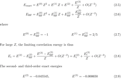
• One in the domain between the He and H nuclei

• Two in the domain between the H and Be nuclei

• Two in the domain to the right of the Be nucleus

As mentioned above, these electrons singly occupy the lowest energy orbitals of their

associated domains.

2.3 Atoms

2.3.1 Hydrogen-like ions

The electronic Hamiltonian of the 1D H-like ion with nucleus of charge Z at x= 0 is

ˆ H=−1

2 d2

dx2 −

Z

|x|, (2.1)

and this has been studied in great detail [69, 76–78, 81, 82]. The eigenfunctions

which are consistent with the impenetrability of the nucleus are

ψ_n+(x) = 2 n

Z n

3/2

xL(1)_n₋₁(+2Zx/n) exp(−Zx/n), x >0, (2.2)

ψ_n−(x) = 2 n

Z n

3/2

xL(1)_n₋₁(−2Zx/n) exp(+Zx/n), x <0, (2.3)

where L(na) is a Laguerre polynomial [100] and n = 1,2,3, . . .. All of these vanish

at the nucleus (which is counter-intuitive) and decay exponentially at large |x|.

Curiously the ground-state energy of the 1D hydrogen atom is−1_/₂_E_h_{, identical to}

that of the 3D hydrogen atom. Additionally, because of nuclear impenetrability, the

ground state of the 1D H atom has a dipole moment andhxi =±1.5.

2.3.2 Helium-like ions

The electronic Hamiltonian of the 1D He-like ion is

ˆ H=−1

2 ∂2 ∂x2 1 + ∂ 2 ∂x2 2 − Z |x1|

− Z |x2|

+ 1

|x1−x2|

(41)

2.3. ATOMS 27

Total energy Correlation energy HF property Ion −Eexact −EHF −EcMP2 −EcMP3 −Ec −Ecsoft Gap

p

hx2_i

1H1– 0.646584 0.643050 1.713 2.530 3.534 39 0.170 2.296 1He1 3.245944 3.242922 2.063 2.688 3.022 14 1.265 0.985 1Li

+

1 7.845792 7.842889 2.235 2.733 2.903 8 3.200 0.628 1Be12+ 14.445725 14.442873 2.335 2.747 2.851 6 5.874 0.460 1B13+ 23.045686 23.042864 2.401 2.751 2.822 9.294 0.364 1C14+ 33.645661 33.642859 2.447 2.752 2.802 13.463 0.301 1N15+ 46.245644 46.242855 2.481 2.751 2.789 18.382 0.256 1O16+ 60.845631 60.842852 2.508 2.749 2.779 24.050 0.223 1F17+ 77.445621 77.442849 2.529 2.748 2.772 30.468 0.198 1Ne18+ 96.045613 96.042847 2.546 2.746 2.766 37.635 0.177

Table 2.1: Total energies (in Eh), correlation energies (in mEh), HOMO-LUMO

gaps (in Eh) and radii (in a.u.) of the 1D helium-like ions. The softened Coulomb

operator of Wagner et al. [48] has been used to obtain the −E_csoft values.

and two families of electronic states can be considered:

• The one-sided AZ₂−2 family where both electrons are on the same side of the

nucleus;

• The two-sided1AZ2−2 family where the electrons are on opposite sides of the

nucleus.

Some of the properties of the first ten ions are gathered in Table 2.1.

One-sided or two-sided?

Because of the constraints of movement in 1D, electrons shield one another very

effectively and, as a result, the outer electron lies far from the nucleus in the A₂(Z – 2)

state. Because of this, the A₂(Z – 2) state is significantly higher in energy than the

1A (Z – 2)

1 state. For example, the HF energies of He2 and 1He1 are −2.107356 and

−3.242922, respectively.

In the hydride anion H– (Z = 1), the nucleus cannot bind the second electron in

the H₂– state and this species autoionizes. The corresponding state of the helium

atom is bound but its ionization energy is only 0.1074. Whereas the minimum

nuclear charge which can bind two electrons isZcrit≈1.1 in the A₂(Z – 2) state, it is

Zcrit ≈0.65 in the 1A (Z – 2)

1 state. In comparison, Baker et al. have reported [101]

that the corresponding value in 3D is Zcrit≈0.91.

In the ₁A₁(Z – 2) state, each electron is confined to one side of the nucleus, and is perfectly shielded from the other electron by the nucleus, assuming that nuclei have