This is a repository copy of The Distribution of Individual Values of Time: An Empirical Study Using Stated Preference Data.
White Rose Research Online URL for this paper: http://eprints.whiterose.ac.uk/2314/
Monograph:
Wardman, M. (1987) The Distribution of Individual Values of Time: An Empirical Study Using Stated Preference Data. Working Paper. Institute of Transport Studies, University of Leeds , Leeds, UK.
Working Paper 244
[email protected] https://eprints.whiterose.ac.uk/ Reuse
See Attached
Takedown
If you consider content in White Rose Research Online to be in breach of UK law, please notify us by
White Rose Research Online http://eprints.whiterose.ac.uk/
Institute of Transport Studies
University of Leeds
This is an ITS Working Paper produced and published by the University of Leeds. ITS Working Papers are intended to provide information and encourage discussion on a topic in advance of formal publication. They represent only the views of the authors, and do not necessarily reflect the views or approval of the sponsors.
White Rose Repository URL for this paper: http://eprints.whiterose.ac.uk/2314/
Published paper
Wardman, M. (1987) The Distribution of Individual Values of Time: An Empirical Study Using Stated Preference Data. Institute of Transport Studies, University of Leeds. Working Paper 244
Working Paper
244June,
1987
THE DISTRIBUTION OF INDIVIDUAL VALUES OF
TIME: AN EMPIRICAL STUDY USING
STATEDPREFERENCEDATA
ITS Working Papers are intended to provide information and encourage discussion on a topic in advance of formal publication. They represent only the views of the authors, and do not necessarily reflect the views or approval of the sponsors.
.-. .
Abstract
Wardman, H. (1987) The Distribution of Individual Values of Time: An Empirical Study using Stated Preference Data. Workinq Paper 244,
Institute for Transport Studies, University of Leeds.
This paper reports the findings of further work undertaken on the Stated Preference (SP) data collected as part of the Department of Transport's Value of Time Project. The latter study estimated values of time in a variety of different circumstances and for a number of modes of travel and also examined how the value of time varied according to socio-economic factors. Although values of time were allowed to vary across individuals by segmenting the data according to socio-economic factors, the SP data permits the estimation of values of time at the individual level whereupon a distribution of
individual values can be obtained.
The Department of Transport expressed some interest in what information could be provided by the SP data about the distribution of values of in-vehicle time across individuals. Individual values of in-vehicle time have been estimated for each of the five SP experiments which had previously been conducted to obtain a distribution for each survey context and also pooled across surveys to derive a population distribution. The problems of estimating values at the individual level with the SP data available are considered and the findings are compared with the average values previously derived in the Value of Time Study. How these individual values of time vary with socio-economic factors is also considered.
Acknowledqement
The findings reported in this paper were obtained from a study of the distribution of individual values of time undertaken for the Department of Transport by MVA Consultancy and Leeds University Institute for Transport Studies. I would like to thank John Bates for the guidance provided in conducting this research and for useful comments on a draft version of this paper.
1. Introduction
After the Final Report on the Value of Time study conducted for the Department of Transport had been presented (MVA et al. 1987), the Department of Transport expressed some interest in what information could be provided about the distribution of values of in-vehicle time in the population. The method of Stated Preference (SP) had been used to estimate values of time and, in principle at least, separate values of time can be estimated for each individual and thus a distribution of values of time can be obtained. In Revealed Preference (RP) models, each respondent contributes a sinqle observation, which precludes any possibility of calibrating individual models. However, SP experiments require individuals to evaluate a number of hypothetical travel scenarios and this presents a possibility of calibrating at the individual level.
It is important to point out at the outset that the SP experiments conducted in the Value of Time Study were
not
designed to estimate separate values of time for each individual. The intention was always to pool individuals together, that is estimate conventional disaggregate models, and bring out the effects of socio-economic variables, which lead to variations in the value of time across individuals, using segmentation analysis (Bates and Roberts 1986). As a result, the number of travel scenarios evaluated by each individual is low for the purposes of calibrating individual models. This leads to difficulties in obtaining precise estimates of time and cost coefficients and, because the value of time is derived as the ratio of the time and cost coefficients, both coefficients must be reasonably precisely estimated if we are to have confidence in the estimated values. Lack of precision in either coefficient can yield extremely high or negative values.Fixed coefficient models, such as the conventional multinomial logit model, assume that there is no variation in tastes across individuals except by explicitly allowing for systematic variations in tastes by segmenting the model accordinq to socio-economic factors. However, this can not discern variations in tastes which are of a purely random nature.
Random coefficient models, such as multinomial probit, allow for variations in tastes and estimate mean values of coefficients along with their variance although at a cost of somewhat greater complexity. Statistical support has been found in empirical studies for random over fixed coefficient models (Daly and Zachary 1975; Fischer and Nagin 1981; Hausman and Wise 1978).
Analysis at the individual level has advantages over the above two forms of disaggregate random utility models in that tastes are allowed to vary across individuals and no a priori restrictions are placed upon the form of the taste variation. Beggs, Cardell and Hausman (1981), referring to the calibration of separate SP models for each individual, conclude that, lathe specification leads to a significant improvement over the specification with identical coefficients1I
.
distributions of values of time in forecasting are discussed in MVA Consultancy (1987).
2. Estimatinq Individual Values of Time
2.1 Review of the Stated Preference Experiments
Five surveys containing SP experiments were c o n d ~ c t e d ~ a s part of the Value of Time project. These experiments required individuals to trade-off between hypothetical levels of relevant travel attributes, from which the relative valuations of these attributes can be deduced. The five surveys were based on North Kent rail and coach commuters, motorists making urban journeys in Tyne and Wear, long distance rail and coach travellers, inter urban car travellers and urban bus users. The precise nature of each survey varied and the main details of each are listed in Table 1.
Table 1: Main Characteristics of the SP Experiments
SURVEY PURPOSE CONTEXT RESPONSE ALTS (1) VARS (2) OBS (3)
NKent Commuting Mode Choice Rating 16 5 1322
Tyne Non Work Route Choice Rating 16 4 1581
LD R/C Leisure Mode Specific Rating 12 4 1272
LD Car Leisure Mode Specific Ranking 10 3 439
Bus Leisure Mode Specific Ranking 10 3 347
Notes: 1) Number of pairwise comparisons or options to be ranked 2) Number of variables describing each travel option
3) Maximum number of observations (individuals) available
The above five surveys effectively contain seven SP data sets which can be analysed to estimate the distribution of values of time across individuals. The Tyne Crossing study examined commuting and leisure travel separately and the Long Distance Rail and Coach SP data sets were also treated separately. For comparability with the results previously derived, these distinctions are here maintained.
In the North Kent SP experiment, where the choice offered was between train and coach, each mode was characterised in terms of main in- vehicle time, other in-vehicle time, walking time, waiting time and cost. The Tyne Crossing experiments described the two routes in terms of the time spent in congested traffic, time spent in free flow traffic, petrol cost and toll charge. The Long Distance Rail and Coach experiments included in-vehicle time and frequency, in the form of different departure timetables, plus maximum possible delay time and fare. These SP experiments all involved pairwise comparisons, and individuals expressed a preference between options in terms of a categorical rating where permissible responses were on a five point scale of: definitely prefer x, probably prefer x, no preference, probably prefer y, and definitely prefer y.
frequency and fare and the second included likely waiting-time, with a range indicating the reliability of the service, in-vehicle time and fare. In both experiments one of the ten options was lcustomisedl to represent the individual's actual journey when initially contacted. Given that we are concerned with the value of in-vehicle time only, the first bus SP experiment can be ignored.
2.2 Methods of Estimation
The methods used for estimating values of time for each individual from the preferences expressed are the same as those used in the initial studies where individual responses were pooled. Modelling the rating responses makes use of the informational content of responses on a five point scale by assigning an arbitrary but sensible probability to each response to denote the likelihood of choosing a particular option. A scale of 0.9, 0.7, 0.5, 0.3, and 0.1 was used in the initial studies to represent the responses of 'definitely prefer option x' through to 'definitely prefer option
Y'
in terms of the probability of choosing option x. These assumptions are maintained here and the values are submitted to a binary logit model of the form:L O ~ [ P ~ / ( ~ - % ) ] = ab
+
at (Xix-
x.,~)+
. .
.
. .
+ a,(XqX-
Xmy)where the explanatory variables represent the attributes of options x and y. The calibration of this model for each individual yields estimates of the coefficients associated with each variable and was undertaken using GLIM (Baker and Nelder 1978).
The exploded logit model was used to analyse the ranked data. The model used was the BLOGIT program of the Australian Road Research Board (Crittle and Johnson 1980), modified to accept ranked data. Thus a model of the following form is estimated for each individual:
5
= exp(uX) /E
exp(uy)Y
The utilities of the travel options are a function of relevant attributes, that is:
and calibration of the model yields estimates of the coefficients of the utility function. The multinomial logit formulation is simultaneously applied to the preference of the first ranked option over the remaining n-1 options, the preference of the second ranked option over the remaining n-2 options and so on until the ranking is exhausted. These modelling techniques are discussed in greater detail in the Value of Time study final report (MVA et al. 1987)
The value of time is derived as the ratio of the estimated time and cost coefficients, and as variations in either of these lead to variations in the value of time, both coefficients must be allowed to vary across individuals to examine the distribution of values of time
.
2.3 Establishing the Methodology
decisions as to the precise methodology to be adopted.
Apart from yielding information on the distribution of values of time, individual analysis also has advantages for the estimation of mean values of time because it can avoid the problems which may arise due to inter-personal taste variations and variations in the functional form of the utility expression across individuals. However, the SP data sets are far from ideal for the purposes of calibrating separate models for each individual, particularly in the case of long distance rail and coach travel and the ranking experiments, due to the relatively limited number of observations per individual. At the design stage, there was no intention that models other than conventional disaggregate models would be calibrated and the number of observations per person is perfectly adequate for this purpose.
In order to increase the chances of obtaining significant value of time estimates for a satisfactory number of individuals, more parsimonious formulations are necessary to obtain the maximum degrees of freedom consistent with allowing both the time and cost coefficients to vary across individuals and avoiding biased coefficient estimates due to the omission of variables relevant to choice.
Initial simplifications are to assume a linear-additive utility function and to constrain all coefficients to be generic, that is to be constant across alternatives. Linear-additive utility functions and generic coefficients have been assumed in the calibrations previously undertaken in the Value of Time study. This latter assumption avoids the need to specify separate coefficients for each option, and thus avoids a reduction in available degrees of freedom. The only case where this may be unreasonable is the North Kent mode choice experiment: here the estimated values of time will reflect averages of alternative specific values of time.
Suppose the SP experiment contains the four travel attributes of cost, in-vehicle time, walk time and wait time which influence travel choice. A linear-additive representative utility function with generic coefficients is therefore specified as:
U = a + a X + a X + a X + a X
0 1 c 2 t 3 wk 4 w t
where the variables denote differences in attributes in the case of pairwise comparisons and absolute attribute values in the case of ranking exercises. There are four basic approaches which we might here use in estimating values of time for each individual.
i) The most general approach is to enter each of the four variables of the SP experiment and an alternative specific constant (ASC) into the calibrated models. This is unlikely to be worthwhile when there are more than two or three coefficients to be estimated given the relatively few choices made by each individual.
ii) In-vehicle time must be allowed to vary separately across individuals but the other time variables could be combined to increase the degrees of freedom. Thus in this example, walk and wait time could be combined into an out-of-vehicle time term, effectively constraining a and a to be the same. Similarly,
these values could be constrained to be some function of in- vehicle time, for example, out-of-vehicle time is taken to have twice the latter value.
iii) A variable can be removed from the equation to achieve greater parsimony. Omitting walk time effectively constrains as to be zero and this might be done if it is found to be insignificant although if the SP experiment is based on an orthogonal design, where the attributes are independently distributed, variables whose coefficients are significant can be removed without affecting the estimates of remaining coefficients. However, omitting the ASC, which is not distibuted independently of the other variables, may influence the remaining coefficients.
iv) Coefficients other than those for cost and in-vehicle time can be constrained to equal the values obtained from the sample of individuals as a whole. This increases the degrees of freedom surrounding the time and cost coefficients but has the drawback that the average values of say walk and wait time are not appropriate for all individuals. When the SP design is orthogonal, constraining a3 and a* to equal average values is essentially the same as constraining them to be zero as the former constraint will also not influence the coefficient estimates of the other variables although overall goodness of fit may be reduced. However, constraining the ASC may influence the other coefficients.
The North Kent, Long Distance Car and Urban Bus experiments employed orthogonal designs, and thus explanatory variables can be omitted or their coefficients constrained without serious consequences in terms of the value of time estimates derived although the use of the exploded logit approach interferes to some extent with the orthogonality property. The Tyne Crossing and Long Distance Rail and Coach designs are not orthogonal although the correlations between attributes are not high in either case.
In order to obtain some insight into the merits of the different approaches, and to assess the feasibility of calibrating individual models, exploratory analysis was undertaken on 50 individuals taken from the North Kent data set. This data set was chosen for preliminary analysis because the SP experiment contained the largest number of explanatory variables and was the only choice context where alternative-specific effects are likely to have a significant influence upon choices. The form of the utility expression for Urban and Inter-Urban Car travellers is much more straightforward given that only in-vehicle time and cost enter the SP experiments and alternative specific effects are unlikely to be a major influence in the former and are not relevant in the latter.
1. U = f(ASC, COST, MIVT, OIVT, WALK, WAIT)
2 . U = f(ASC, COST, IVT, OVT)
3. U = f (ASC, COST, IVT) 4. U = ffCOST. IVT)
where MIVT, OIVT, IVT and OVT are main in-vehicle, other in-vehicle, in-vehicle and out-of-vehicle time respectively.
The models range from the most general permissable, where each attribute is entered separately along with an ASC, to the most restricted given that COST and MIVT/IVT must vary across individuals. The effect of omitting variables, combining variables and restricting the coefficients to the overlall averages are all considered.
As expected, the first model was found to be clearly impractical. Of the 5 0 individuals considered, 16 were found to have only two siqnificant coefficients, 18 had only one significant coefficient whllst 7 had no significant coefficients. Fortunately the coefficients of MIVT and COST were most frequently significant.
Combining variables into OVT and IVT proved to be an improvement over the more general form for 4 9 of the 5 0 individuals according to F tests although OVT was significant in only five cases. Given this latter finding, a further improvement was not surprisingly obtained for all but these five individuals when OVT was omitted.
Omitting the ASC as was done in model 4 appeared to worsen the models in general and also influenced the time and cost coefficients. With the exception of the MIVT and COST coefficients, the ASC was the most frequently significant coefficient in the least restricted formulation of model 1.
Comparing models 5 and 3 revealed the former model, incorporating MIVT instead of IVT, to be a slight improvement although the differences in the derived values of time were not large.
Turning to the constrained models, the formulation with MIVT (model 7) was preferred to that with IVT (model 6) in 36 of the 5 0 cases which is a finding similar to the unconstrained models. Although constraining WALK and WAIT has no effect on the value of time in relation to the unconstrained models where WALK and WAIT are omitted, due to the orthogonal design, better fits were generally obtained and the values of time were estimated with greater precision.
Although this exploratory analysis was based on the North Kent data set, and determines a preferred model for the analysis of this data, some conclusions can be made regarding the likely problems to be faced, the feasibility of deriving values of time from individual calibrations in these circumstances and the relative merits of different approaches.
Entering all the variables of the SP experiment into the calibrated models is not worthwhile when the number of coefficients to be estimated exceeds two or three given the few observations per person. The significance of the value of in-vehicle time, which is the relative value of interest here, can be increased using more parsimonious formulations.
Constraining coefficients - to average values is potentially
inappropriate, although not when orthogonal designs are used, but improved fits and values of time with greater significance were obtained in this initial analysis using such an approach.
Omitting significant coefficients when the design is not orthogonal is not appropriate but omitting variables whose coefficients are insignificant improves models. However, such an approach would require the identification of those individuals who have insignificant coefficients and recalibration of the models. Variables should be combined wherever appropriate to increase degrees of freedom.
It will be possible to estimate significant values of time for some individuals, even with these limited data sets, but it is clear
that
this will not be possible for all individuals and indeed there may be a relatively large proportion for whom the value of time can be estimated with much less significance than is commonly regarded as acceptable.This suggests that the criteria for evaluating significant values will have to be revised to consider values of time which are significant at levels of confidence less than the customary 95%. It will be necessary to examine the consequences of such actlon on the distribution of values of time across individuals and on the plausibility of the values of time derived.
The best model overall is not necessarily the best for each individual. Improvements could be obtained if individuals were allowed to have different functional forms of representative utility expression or if, for any given functional form such as the linear additive used here, the best model along the lines of those listed above is identified for each individual. Such an approach was not feasible within this study.
3. Findings Concernins the Distribution of Values of In-Vehicle Time
3.1 General Discussion
In the experiments which involved the rating of travel alternatives, those individuals whose responses were the same for all comparisons, and for whom a model can not therefore be calibrated, were omitted from consideration. In general, this led to the omission of around 10% of individuals. In the vast majority of cases where this arose the responses were of the form of a definite preference. No equivalent criterion exists in the case of ranked data. In the Value of Time project, individuals were omitted from consideration if their responses followed some identifiable pattern such as always choosing the quickest option as preferred or if they appeared to contain serious irrationality. Such responses were interpreted as being inconsistent with the underlying assumptions of the models used or as containing serious error.
These latter criteria have-not been usedhere. It was considered preferable to avoid omitting such individuals given the anticipated problems of estimating sufficiently precise values of time for a satisfactory number of individuals. The results derived in the previous studies were largely insensitive to such omissions although it is more likely that poor models are in any event calibrated for these individuals.
The following discussion is based on the results derived for North Kent commuters but these are qenerally of a similar nature to those obtained for the other experiments. It will be recalled that the preferred North Kent model was based on constrained values of OIVT, WALK and WAIT but MIVT, COST and ASC varied across individuals.
Figure 1 presents the absolute frequency distribution of values of in-vehicle time for the North Kent experiment in a range from 0 to 12 pence per minute in bands of 0.5 pence per minute. Three distributions are qiven reflecting: a) all individuals, b) those with a value of time significant at the 60% confidence level and c) those whose value of time is significant at the usual 95% level. Clearly, the number of individuals falls as the criterion for inclusion becomes more strict, so that the lowest distribution represents only those values of time significant at 95%.
Also reported in Figure 1 for each level of significance are the mean value of time, the standard deviation of the values of time, the standard deviation of the mean value of time (standard error), the number of observations, the maximum value of time, the number of negative values of time and the number which were twelve pence per minute or more. The frequency distributions and summary statistics for each level of significance for the other SP experiments are given for reference in appendix 1.
A notable feature of the North Kent results is that the 95% significance criterion omits a large proportion of individuals, as expected. This was also apparent in the other experiments although generally to a lesser extent. It would seem preferable to use a less stringent criterion in interpreting what is and is not a value of time estimated with sufficient precision.
pence per minute. Many of the latter are unrealistcally large, reaching a maximum of 189.50.
The cause of such extreme values is that either the time or the cost coefficient is poorly estimated. The time or cost coefficient can be so poorly estimated as to be negative which results in negative values of time whilst an imprecisely estimated cost coefficient can lead to a very high implied value of time. If an individual's responses contain a large amount of error so that there is no real relationship between preferences and travel attributes, the time and cost coefficients are likely to be small. This may lead to a relatively large number of low values of time in addition to negative or very large values.
60% confidence, roughly corresponding to a confidence interval of plus and minus one standard-deviation and to a t ratio of one, was examined as an alternative criterion for omitting individuals. The extremes apparent when all individuals are included are avoided, but without the large effect on sample sizes which results from the imposition of a 95% confidence level. It was found that the 60% confidence level omitted all negative values of time and a large number of the extreme positive values of time whilst avoiding the omission of a large number of plausible values. The mean value of time does vary between the 60% and 95% confidence sets but the difference is not unduly large. Similar results were found in all the SP experiments.
In terms of the distribution of values of time in the range from 0 to
12 pence per minute, the pattern is roughly similar across the three different acceptance criterion with the exception of very low values of time which are discussed below. This was also found to be the case in the other experiments.
It would seem, therefore, that a more appropriate criterion for omitting an individual is whether the estimated value of time is significant at a 60% level of confidence.
Another feature common to all the experiments is the relatively large proportion of individuals who are omitted by the 60% and 95% significance criteria at very low values of time. This was a cause for some concern as for a given standard deviation a value of time will be more significant at higher levels. This would seem to discriminate against low values of time. Analysis was undertaken to examine whether low values of time were being discriminated against.
Consider the relationships between the standard deviation of the value of time and the value of time itself depicted in Figure 2.
Line A denotes a proportional relationship between the value of time and its standard deviation and in this case is a 45 degree line which corresponds roughly to our 60% acceptance criterion. Thus at any point below this line, the t statistic of the value of time exceeds one and is regarded as significant. If the relationship is proportional, regardless of whether it is one-to-one, a value of time
is equally likely to be significant at low values as high values.
Line B represents a relationship where the standard deviation falls as the value of time increases. In the particular example used, relatively low values of time will be insignificant. Some individuals' responses may contain such error that there is no clear relationship between preference and the explanatory variables. In such instances, the estimated coefficients will be small and the value of time estimates may also be low and will be estimated with large standard errors. The low values of time derived will be associated with relatively high standard errors. However, this does not discriminate against low values of time as they would be omitted due to their relatively high standard deviations.
It is in the case depicted by line C, where the standard deviation does not vary much with the value of time, that values of time will be omitted as insignificant when they are low precisely because they are low and any significance level becomes a stricter test at low values of time.
For each experiment, the distribution of estimated standard deviations in bands of 0.25 pence per minute was obtained for each of the value of time bands considered. The average standard deviation in each band was also estimated.
For a range of values of time up to around five pence per minute, the standard deviations fell as the value of time increased in both sets of Tyne Crossing results and also, but less distinctly, for the Long Distance Coach results whilst the standard deviations appear to increase with the value of time in the North Kent results. In the Inter Urban Car and Long Distance Rail experiments the relationship appears to be constant but no clear relationship is apparent for Urban Bus given the relatively few observations involved.
Given that some very low values of time have standard errors which compare favourably with hiqher values of time, it was decided to adjust the acceptance criterion to include those values of time which were estimated with a standard deviation of 0.5 pence per minute or less in addition to the 60% significance criterion. This additional criterion clearly does not have any effect on the frequency distribution other than at the lowest value of time band. All further distributions reported below are based on these acceptance criteria.
3.2 North Kent
The frequency distribution for the North Kent results is presented in Figure 3 in the same manner as for Figure 1 except that only one distribution is supplied according to the criteria outlined above. The same summary statistics are also given.
The raw data set contains 1322 individuals who had supplied adequate SP information. This is reduced to 1198 individuals after omitting those whose responses exhibited no variation and is further reduced by excluding the 39 individuals for whom the value of time is undefined, that is where the cost coefficient is zero. 749 of the remaining 1159 individuals for whom a value of time could be estimated satisfied the acceptance criterion.
A feature of the North Kent results which is not apparent in the other studies are the peaks in the frequency distribution. These occur in the value of time bands of 2.5 to 3 and 4 to 4.5 pence per minute and also to a lesser extent in the 8 to 8.5 pence per minute band. These points were identified as being boundary points in the experimental design
-
that is, values of time which represent a point of indifference between options. These appear to have increased the number of individuals who have values of time in these bands although it would seem unreasonable to infer that these additional individuals have values of time far removed from those estimated whilst a uni- modal distribution might peak in the lower or even the middle of these three value of time bands.This was the first SP experiment conducted in the value of time project and with hindsight it could have been improved by
incorporating a larger ranqe of boundary values of time. These design limitations do not arise in the other SP experiments where detailed attention was paid to ensuring that the values of time implied by the time-cost trade-offs provided a realistic range of boundary values of time
.
Interpreting the distribution is made more difficult due to the peaks caused by the design. The general trend appears to be that the distribution is skewed to the right as might be expected. The mean value is such that the range of plausible values of time would extend farther for higher than average values than lower than average values of time. Assuming that the first peak is the true peak, albeit an exaggerated one, and ignoring the other two peaks as being a result of the design, the distribution rises sharply at low values of time and reaches a peak at a value less than the mean value. It falls quite sharply from the peak but the rate at which it falls diminishes as the value of time increases.
The mean value of time is somewhat hiqher than the value of main in- vehicle time of 2.94 derived from a single model calibrated for on individuals. Allowing for the standard deviations of the estimates, the two values are highly significantly different (t=6.54).
The distribution of the constrained ASC model is much smoother than the unconstrained model and is very steep at values of time surrounding the peak. There are an additional 228 individuals who satisfy the acceptance criteria in relation to the unconstrained ASC model and there were no cases where the value of time was undefined. The mean value of time at 3.07 is also much closer to the single value derived from the overall calibration and the two are
insignificantly different (t=1.01).
3.3 Tyne Crossing
The Tyne Crossing commuting and leisure raw data sets contained 1027 and 554 individuals respectively. These were reduced to 936 and 487 after omitting those whose SP responses were always the same. There were no instances where the value of time was undefined and 600 commuters and 302 leisure travellers had values of time which satisfied the criteria for inclusion.
The form of the utility function is more straightforward in this case. It is unlikely that there are strong alternative specific effects and thus the ASC can be omitted without serious consequences. In the previous study, petrol cost and toll charge were found to have different utility effects although the differences were not large and it would not seem unreasonable to combine the two.
The value of delay time was previously found to exceed the value of free time by a factor of about 40%. These two attributes could be considered separately but they would qenerally be estimated with less precision than a combined time variable and thus the latter was entered into the calibrated models. The Tyne Crossing commuting and leisure models therefore contain 16 observations and only two variables. Models which included ASC1s were also calibrated but this was found to have a negligible effect upon the frequency distributions and the mean values obtained.
The frequency distributions for the commuting and leisure data sets are given in Figures 5 and 6 along with summary statistics. The distributions again appear to be skewed to the right as might be expected. There are no negative values of time and relatively few which are in excess of twelve pence per minute.
The overall values of time derived from the models estimated on the pooled data, after taking averages of the values of delay and free time defined in terms of both petrol and toll costs, were 3.79 and 4.88 for commuting and leisure trips respectively and these are similar to the mean values obtained from the indivxdual calibrations of 4.19 and 4.64.
3.4 Long Distance Rail and Coach
The modelling process is here more restricted than for the above experiments as each individual undertook only 12 pairwise comparisons of travel options. Given that the experiment required the evaluation of mode specific travel scenarios, there is no reason to include an ASC. However, two variables in addition to in-vehicle time and cost characterise each option.
The calibrated models were of the same form as for the North Kent experiment. The delay and frequency coefficients were constrained to equal the average values derived in the previous studies. These two variables cannot be omitted without influencing the in-vehicle time and cost coefficients as the design is not orthoqonal although constrained formulations provided more precise estimates in the exploratory analysis. The inclusion of all four variables is hardly likely to be worthwhile.
The frequency distributions and summary statistics for the two data sets are given in Figures 7 and 8. Neither distribution is particularly smooth but, unlike the North Kent experiment, this is not considered to be a result of the experimental design as a reasonable range of boundary values of time was implied by the design. It would seem that this is more a chance occurence and the distributions could be made smoother by rearranging the value of time bands.
The distributions are also less concentrated around the peak than for the North Kent and Tyne Crossing experiments but they do appear to be skewed to the right. Again there are no negative values of time but there are a relatively large number of values of time in excess of twelve pence per minute.
The mean values of in-vehicle time for the rail and coach experiments are 5.42 and 5.76 respectively. That the latter exceeds the former is surprising, even though coach travel has a higher disutility, given the tendency for those with higher values of time to choose the quicker option of train. The values of time obtained from the pooled data calibrations were 6.00 and 3.90. The values derived by the two methods are insignificantly different for rail travel (t=1.03) but the coach values are quite different and this difference is significant (t=6.36). The standard deviation of the value of time tended to fall as the value of time increased for coach users and thus a relatively large proportion of very imprecisely estimated low values of time have been excluded according to the significance criteria. This will have increased the mean value obtained from the individual calibrations and seems to have under-represented the number of individuals in the lower parts of the frequency distribution.
3.5 Inter Urban Car
The utility function to be estimated is straightforward in this case. As only time and cost enter the design, and these must both be allowed to vary across individuals, factors other than the time and cost variables are not relevant. Given that only ten scenarios were evaluated by each individual, the separate consideration of the two forms of time would most likely lead to values of time which are poorly estimated for a large number of individuals. Thus the two time variables were combined into a single time term.
The raw data set includes 439 individuals and 427 of these had supplied a complete ranking of the travel options. The iterative modelling procedure did not converge for 56 individuals, largely as a result of lexicographic orderings of the options in terms of total time and rankings which appeared to contain serious irrationalities. Lexicographic orderings based on toll charge did not result in a failure of the model to converge but yielded negative values of time with very low t ratios. 234 of the remaining 371 had values of time which were estimated sufficiently precisely.
The frequency distribution of the value of in-vehicle time for long distance car travellers is given in Figure 9. The distribution is again not particularly smooth although it is not considered to be the result of a design limitation. The distribution appears to be skewed to the right. It rises sharply to the first peak and generally tails-off quite steadily across a wide range of values of time.
The value of time derived from the previous modelling work where all the individuals were pooled was 3.8 pence per minute. The mean of the values derived at the individual level at 4.61 is somewhat higher than the latter value even though negative values of time are included.
3.6 Urban Bus
The Urban Bus SP experiment required individuals to rank ten alternatives in order of preference and these alternatives contained in-vehicle time, likely waitinq time and fare. One of the travel options was lcustomisedl and depicted the individual's actual journey when initially contacted.
The nine options which had common attributes across individuals followed an orthogonal design. Although the inclusion of the lcustomisedl options results in non-zero correlations between attributes, these correlations remain very low. Thus wait time was not included in the estimated models. An ASC was not included to represent any tendencies to prefer the current situation as this current situation is only represented in one option.
The raw data includes 347 individuals and 261 had supplied adequate information regarding the journey made when initially contacted and had completed the ranking exercise. The model did not converge in 22
cases and 122 of the remaining individuals had values of time which were estimated sufficiently precisely.
of individuals with low values of time. Although the distribution tails-off very gradually after a sharp drop from the low value of time groups, there are few individuals in the higher ranges of the distribution.
The mean value of time obtained is 1.68 and this is essentially significantly different (t=1.98) from the value of time of 1.28 derived from the pooled data. This is so despite the inclusion of negative values of time and 13 very low values of time which are insignificant but which have standard deviations of 0.5 or less, and the absence of very large values of time. However, the difference is not particularly large.
4. The Distribution of Population Values of In-Vehicle Time
The distribution of the value of time in the various experiments is generally consistent with what would be expected. Table 2 lists the coefficients of variation to enable a comparison of the variation in the values of time across experiments when the mean values of time differ. The coefficient of variation is calculated as the ratio of the standard deviation of the values of time and the mean value of time
.
Table 2: coefficients of Variation
North Kent (1) 1.01 Long Distance Rail 0.67 North Kent (2) 0.61 Long Distance Coach 0.69
Tyne Commuting 0.79 Long Distance Car 1.41
Tyne Leisure 0.69 Urban Bus 1.26
Notes (1) Unconstrained ASC (2) Constrained ASC
There is typically a considerable spread in the value of time across individuals. Some of this will be due to identifiable factors such as socio-economic variables and trip characteristics but some wjl? also stem purely from random variations in preferences across individuals. The extent of variation in the value of time is very similar for North Kent commuters, using the constrained ASC model, urban car travellers and long distance rail and coach users but it is not constant across all contexts. The variation is somewhat higher for urban bus users, long distance car travellers and North Kent commuters if the unconstrained ASC model is taken to be more appropriate.
MODE HH SIZE STATUS INCOME
Car One Student (16+) -5000
Bus Two Retired 5-10000
Rail Three+ Other Adults 10-15000
Coach 15-20000
20000+
There are problems in using NTS data as a representative measure of the travel and socio-economic characteristics of the overall population. Amongst these are that the most recent data available was collected in 1978/79 and thus the data for long distance bus/coach, in which category North Kent coach commuters were placed, does not represent the effects of the deregulation of long distance bus services in 1980 whilst other travel patterns may have changed over this period, for example, due to increasing car ownership. The distribution of socio-economic characteristics may also have changed. However, NTS data was the best available for comparison purposes.
There are also shortcomings in interpreting the sample of individuals obtained as potentially representative of all travellers given that car passengers were not surveyed and because of factors such as restricting the urban bus survey to travellers making journeys for private travel purposes. Some allowance could have been made for car passengers although they do not necessarily have the same value of time as car drivers, for example( if time spent driving and being a passenger do not incur the same disutility. However, we do not expect the difference to be large. Taking those making journeys by bus for private travel purposes to represent all bus users implicitly assumes no variation in the value of time between commuting and private travel but it would not seem unreasonable to assume that the value of time does not vary by a large amount on this account.
Allowance must be made for some different characteristics of the North Kent survey. The income question was based on personal rather than the household income of NTS and the other surveys and the income groups used were different to the latter surveys. The survey was also undertaken in 1983 and thus adjustments must be made for inflation to achieve comparability with the other surveys which were conducted in 1985.
After omitting those who had not supplied relevant socio-economic information, and also those whose value of time did not satisfy the significance criterion, the sample sizes were 1083 for car, 694 for rail, 506 for long distance bus and only 97 for urban bus. The maximum number of 45 categories were initially compared for each mode but the number was subsequently reduced due to the inevitably few observations in many cells.
In the case of car travel, relatively few were students or retired and thus the distinction of employment status was not maintained. The highest two income groups were also combined. Thus 12 categories remained, each with a satisfactory number of individuals. Only limited segmentations were worthwhile in the case of the 97 bus users and the sample was categorised into three income groups only, the largest being £10000 and over.
the same bands as the other surveys, and this required assumptions to be made, the categorisation by income was excluded. The retired and
students were also combined to avoid unduly small frequencies in some cells. Thus both rail and coach travellers were compared with the population of such travellers in terms of only six categories.
Over the four modes, 27 categories were used in weighting the sample of travellers to represent the population of travellers. The scale
factor adjusts the proportion of travellers in a cell in the sample obtained to reflect the proportion in that cell in the NTS data.
It was apparent that the sample proportion of bus users was a large underestimate of the population proportion. This is hardly surprising given that 97 bus users out of a total of 2380 individuals does not reflect the relative importance of bus travel. For the three income groups, the samples were respectively weighted by approximately six, eight and ten.
Rail and coach users appeared to have been oversampled, in some categories by a large amount. This is to be expected given the large survey emphasis on rail and coach travel in relation to their practical importance. The car sample seems to be more representative of the overall population, that is the weights were nearer one than in the previous cases.
Figure 11 presents the relative frequency distribution of values of time estimated for the population of travellers. The distribution is again skewed to the right and seems to reflect the underlying distributions from which it is obtained. It peaks at a relatively low value of time which seems to be due to the relative importance of bus travel and the very low values of time for bus users. The distribution is comparatively smooth and falls quite sharply from its peak until it flattens out at low relative frequencies at values of time of about six pence per minute and over. The relative frequency distribution varies little if the range across which it is specified is made somewhat narrower, for example, up to a maximum value of time of six pence per minute.
The mean value of in-vehicle time across the whole population is estimated to be 3.60 pence per minute and the values of time have a standard deviation of 3.88. The mean value for those with values of time between zero and twelve only, as in the frequency distribution, is 3.44 with a standard deviation of 3.01. These mean values are consistent with the mean values previously derived. They are less than those obtained for each mode except bus although they are not greatly different. The relative importance of bus travel and the low value of time for bus users reduces the mean value of time from the relatively high level associated with other modes.
5. Correlations with Socio-Economic Factors
The values of time derived at the individual level can be combined into groups as appropriate to consider how the value of time varies with socio-economic factors and trip characteristics. Additionally, it is possible to explore variations in the value of time by regressing the value of time on dummy variables reflecting whether the individual is in a particular category or not. This latter approach takes into account variations in the value of time according to a number of categories simultaneously. This is not readily achieved using the former approach as the large number of categories likely to be involved will result in relatively few observations in many categories.
Grouping individuals into categories according to such factors as income, employment status and journey purpose was undertaken. The cateqories considered were largely those which had previously been considered in the segmentation analysis carried out in the Value of Time project. Across all the data sets, 58 stratifications by socio- economic variables were examined.
The results derived for the large number of segmentations undertaken are not discussed in detail here. Instead the more important and interesting findings will be reviewed although the results of the analysis were largely disappointing.
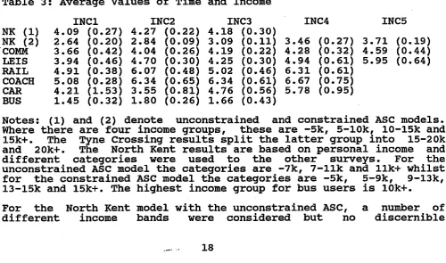
For each experiment, Table 3 lists the average value of time in each income group along with its standard error. It can be seen that the variation in the value of time within income groups is high in relation to the between group variation. This was also apparent in the other segmentations undertaken. These segmentations control for variations in the value of time due to income but variations in other socio-economic factors and random variations in values of time lead to within group variation.
Table 3: Average Values of Time and Income
INCl INC2 INC3 INC4 INC5
NK (1) 4.09 (0.27) 4.27 (0.22) 4.18 (0.30)
NK (2) 2.64 (0.20) 2.84 (0.09) 3.09 (0.11) 3.46 (0.27) 3.71 (0.19) COMM 3.66 (0.42) 4.04 (0.26) 4.19 (0.22) 4.28 (0.32) 4.59 (0.44) LEIS 3.94 (0.46) 4.70 (0.30) 4.25 (0.30) 4.94 (0.61) 5.95 (0.64) RAIL 4.91 (0.38) 6.07 (0.48) 5.02 (0.46) 6.31 (0.61)
COACH 5.08 (0.28) 6.34 (0.65) 6.34 (0.61) 6.67 (0.75) CAR 4.21 (1.53) 3.55 (0.81) 4.76 (0.56) 5.78 (0.95) BUS 1.45 (0.32) 1.80 (0.26) 1.66 (0.43)
Notes: (1) and (2) denote unconstrained and constrained ASC models. Where there are four income groups, these are -5k, 5-10k, 10-15k and
15k+. The Tyne Crossing results split the latter group into 15-20k and 20k+. The North Kent results are based on personal income and different categories were used to the other surveys. For the unconstrained ASC model the categories are -7k, 7-llk and ilk+ whilst for the constrained ASC model the categories are -5k, 5-9k, 9-13k, 13-15k and 15ki. The highest income group for bus users is 10k+.
[image:32.595.67.568.470.765.2]relationship between the value of time and income was apparent even with only three income groups. The position is quite the reverse when the ASC is constrained to equal the average value. There is a monotonic relationship between the average value of time and income across five income groups but although the pattern is clear the effect of income is not particularly strong.
There is also a clear income effect apparent in the Tyne Crossing results although again the effect is not particularly strong. In the segmentation analysis previously undertaken using single models, income was found to have a highly significant but not particularly strong influence on the value of time.
There is also a tendency for the value of time to increase with income in the three long distance travel studies along the lines apparent in the previous studies. The results for urban bus are disappointing. A number of different income groups were considered, although the analysis is restricted by the relatively small sample size, but no clear relationship emerged.
The results of the overall segmentation analysis were generally disappointing although the most significant findings previously obtalned for long distance rail and coach travel resulted from segmentations of the delay and frequency variables and segmented analysis of the urban bus values of time is limited by the relatively few individuals involved. Where clear trends did emerge, they tended to confirm the results previously derived but the level of within group variation is relatively high in all experiments.
As far as some other key variables are concerned, housewives, the unemployed and the retired all had lower than average values of time in the case of urban leisure trips b u t t h e differences were not large. These values are expected to be lower given that such individuals generally have fewer constraints on their available time. The value of time of 3.38 for those retired in the long distance car study is somewhat lower than the average value of 4.61. The retired and unemployed had similar values to the average in the case of long distance rail travel but for coach travel the retired had slightly higher than average values and the unemployed had values which were about one pence per minute below average.
The mean values of time for urban car commuters using the Tyne Tunnel and Tyne Bridge are 5.08 and 3.43 respectively. In the case of leisure travel, the values are 5.82 and 3.81. The differences are quite large and are consistent with the Tunnel attracting those with higher values of time as it is generally the quicker and more expensive route. However, the value of time for North Kent train users is 4.22 and for coach users is 4.16 despite the train being generally quicker and more expensive.
The calibrated models included a constant and n-1 dummy variables for each relevant socio-economic factor containing n categories. Thus the estimated coefficients represent the incremental effect on the value of time of a particular variable at a certain level. The socio- economic variables examined were income, age, sex and the nature of work hours, which were previously found to have a significant influence on the value of time, and also the mode used in practice. The results obtained were very poor. The constant was the only significant coefficient even after omitting or combining several of the most insignificant coefficients and the goodness of fit was extremely low. Given these very poor results for North Kent commuters, it was not considered worthwhile extending the analysis to examine the other data sets.
-
6. Summary and Conclusions
This paper has been concerned with reporting the findings regarding the estimation of individual values of in-vehicle time for the five SP experiments which were conducted as part of the Department of Transport's Value of Time project. Although the SP data is not ideal for the purposes of calibrating individual models, it has proved possible to develop individual models with plausible values of time and obtain distributions of values which seem reasonable for each survey.
The distributions obtained are generally skewed to the right, as might be expected, and the findings are evidence that there is considerable inter-personal taste variation. However, there is a generally high correspondence between the average values of time derived at the individual level and the mean values obtained from data pooled across individuals.
References
Baker, R.T. and Nelder, J.A. (1978) 'The GLIM System Manualr Numerical Algorithms Group, Oxford.
Bates, J.J. and Roberts, M. (1986) 'Value of Time Research: Summary of Methodology and Findings1 Proceedings of Seminar M, PTRC Summer Annual Meeting, Brighton.
Beggs, S., Cardell, N.S. and Hausman, J. (1981) 'Assessing the Potential Demand for Electric Carsr Journal of Econometrics, Vol. 16, pp. 1-9.
Crittle, F.J. and Johnson, L.W. (1980) 'Basic Logit (BLOGIT) Technical Manualr ATM No.9,~Victoria1 Australia.
Daly, A.J. and Zachary, S. (1975) 'Commutersr Values of Timer Report T55, Local Government Operational Research Unit, Reading
Fischer, G.W. and Nagin! D. (1981) 'Random versus Fixed Coefficient Quanta1 Choice Models' in Manski, C.F. and McFadden, D. (eds.) Structural Analysis of Discrete Data with Econometric Applications.
Hausman, J.A. and Wise, D.A. (1978) ,A Conditional Probit Model for Qualitative Choice: Discrete Decisions Regognising Interdependence and Heterogeneous Preferences1 Econometrica 46, pp. 403-426.
MVA Consultancy (1987) 'Report on Distributions of Values of Time' Prepared for APM Division, Department of Transport, Unpublished.
w
k q x 3 - q d i s c r * d x w * ~ n r r b a r a € i r d i ~ i n E a d . l ~ ~ francfl-alfawprrrdmrt-e. %sumarystah&m
. .
z e r o t o W ~ ~ p m ~ p r m i ~ t e i n ' '. 's ard F m p - q distrkutiicrs are fear tk t h e m t q r k d: a) all irdivicbls b) irdivicbkwithestirratEddLES d t i r r e s i ~ b m t a t t k M Y b ~ c f c r n f m c ) irdivicblswith