Progress in the PRIDE technique for rapidly comparing protein three dimensional structures

Open Access

Project Note

Progress in the PRIDE technique for rapidly comparing protein

three-dimensional structures

Svetlana Kirillova

_{and Oliviero Carugo*}

Address: 1_{Department of Biomolecular Structural Chemistry, Programme of Structural and Computational Biology, Max F. Perutz Laboratories,}

Vienna University, Campus Vienna Biocenter 5, A-1030 Vienna, Austria and 2_{Department of General Chemistry, Pavia University, Viele Taramelli}

12, I-27100 Pavia, Italy

Email: Svetlana Kirillova - [email protected]; Oliviero Carugo* - [email protected] * Corresponding author

Abstract

Background: Accurate and fast tools for comparing protein three-dimensional structures are necessary to scan and analyze large data sets.

Findings: The method described here is not only very fast but it is also reasonable precise, as it is shown by using the CATH database as a test set. Its rapidity depends on the fact that the protein structure is represented by vectors that monitors the distribution of the inter-residue distances within the protein core and the structure of which is optimized with the Freedman-Diaconis rule.

Conclusion: The similarity score is based on a χ2 _{test, the probability density function of which} can be accurately estimated.

Findings

Although numerous methods for comparison protein three-dimensional (3D) structures were designed, we still lack a unique, commonly accepted procedure to measure the structural diversity between proteins [1]. In particular, the structures of distantly related proteins should be expressed by the appropriate way allowing their compari-son and the 3D structure representations used in modern algorithms are described in the reviews [2,3]. The most accurate protein structure comparison methods produce protein structure alignments that are computationally intensive. Slower techniques may be preferable to analyze and classify sufficiently small data sets. However, the time criterion is crucial in the case of integrated survey of large databases, like the Protein Data Bank or the domain col-lections CATH and SCOP [4]. This problem is very similar to that encountered few years ago in the case of macromo-lecular sequence databases, which was solved by the

development of tools like FASTA [5], BLAST [6] or PSI-BLAST [7] that allow one to effectively scan enormous databases like UniProt [8], which presently contain sev-eral millions of entries. Although protein 3D structure databases are still much smaller, several representations of protein structure suitable for rapid comparison without alignment were proposed [9-13]. One of the fast and auto-matic techniques for protein structural comparison is PRIDE [9]. In this method the protein structure is repre-sented via a series of distributions of inter-atomic dis-tances allowing the use rapid comparison procedure without alignment.

In the present communication, some improvements of the original PRIDE technology are presented. They make it more accurate than the original version without decreas-ing its speed. The classification ability of the method was tested on the CATH database.

Published: 11 July 2008

BMC Research Notes 2008, 1:44 doi:10.1186/1756-0500-1-44

Received: 25 February 2008 Accepted: 11 July 2008

This article is available from: http://www.biomedcentral.com/1756-0500/1/44 © 2008 Kirillova and Carugo; licensee BioMed Central Ltd.

The PRIDE methodology

In original PRIDE version, a protein structure in defined

by the distributions of the distances between Cαi and

Cα(i+n) atoms, where n, which ranges from 3 to 30, is the

number of C_αatoms between them in the backbone joint.

The comparison between two protein 3D structures is reduced to the comparison between distributions of inter-residue distances. This is performed by chi-square contin-gency table analysis, which estimates whether two distri-butions represent the same overall population and allows one to compute a probability of identity P, ranging from 0 and 1. Since 28 pairs of histograms are compares, 28 P values are obtained and then averaged to give the overall PRobability of IDEntity (PRIDE) between the two protein 3D structures. Such a similarity score can range, by defini-tion, from 0 to 1, the latter value indicating the identity between the two protein structures. In the next sections, four modifications, introduced into this computational procedure, will be described.

Amount of structural information

The maximal value of n, which was equal to 30 in the old PRIDE version, is now selected as a function of the protein dimension. Obviously, the histograms, in which inter-res-idue distances are binned, must have a sufficiently high number of observations to be compared via any statistical tool. The number of observations in the histograms increases with the length of the protein and decreases with n. Therefore, histograms were generated for all n values larger than 3 and lower than n_max, where n_max is the value for which there are only 20 Cαi-Cα(i+n) distances. Clearly, if

n > n_max, the histograms would contain less than 20 obser-vations and they were thus ignored. Therefore, the num-bers of histograms are different for proteins of different length in the modified PRIDE version. In the comparison of two domains, represented by series of Cαi-Cα(i+n)

histo-grams, with 3 ≤ n ≤ n_max1 for the first domain and 3 ≤ n ≤ n_max2 for the second domain, the maximal value of n (nmax) was defined as

n_max = min(n_max1, n_max2)

Moreover, only distances between residues belonging to helices and/or strands were taken into account in the modified PRIDE version, in order to increase the compu-tational speed of the method. The STRIDE package, based on the detection of hydrogen bonds patterns and back-bone torsions, was used for secondary structure assign-ment [14].

Optimization of the dimension of the histogram intervals

The building of a regular histogram from continuous data demands a cautious specification of the number of bins. In the old version of PRIDE, each bin width was arbitrarily set to 0.5 Å, and adjacent bins were merged together so

that at least 5% of the observations were included in each bin. Here a more rigorous approach was followed. Firstly, inter-residue distances were binned in the histograms with a fixed bin width of 0.1 Å, a value close to the average expected uncertainty of protein atomic coordinates obtained with crystallographic methods [15]. Then bin widths are changed automatically to their optimal value BS by using the Freedman-Diaconis rule [16]

BS = 2iqr(x)k-1/3

where k is the number of observations in the sample x; iqr(x) is the interquartile range of the data of sample x, that is the range between the third and first quartiles. The iqr is expected to include about half of the data. The opti-mal BS values are computed for a query protein structure, and then they are used to change the histogram bins for all domains in the scanned database. New optimal BS val-ues must be recomputed for a new query. Despite this might seem to be rather complicated and time consum-ing, we verified that once the histograms for the entire database are pre-computer and stored with very small bins of 0.1 Å, all of them can be re-shaped to the optimal BS very rapidly (see the paragraph "Computational speed" below).

Distribution comparisons

While in the original version of PRIDE, the Cαi-Cα(i+n)

dis-tance distributions were compared using the contingency tables [17], another statistical procedure is applied now. Contingency tables are more suitable to analyze relation-ships between nominal (categorical) variables and can be applied to compare continuous distributions only by care-fully selecting an arbitrary bin size in such a way that each bin contains sufficient data. Here we adopted another approach that is more suitable to compare continuous distributions and that is computationally not more demanding than the contingency table analysis. By assuming that the distributions of both binned data sets of inter-residue distances are equally unknown, it is possi-ble to use the chi-square test to disprove the null hypoth-esis that the two data sets can be described by the same distribution. If R_i is the number of observations in bin i for the first protein and Si is the number of observations in

the same bin i for the second protein, then the chi-square statistics is

where

χ2

2

=

− ⎛

⎝

⎜ ⎞

⎠ ⎟ +

∑

S R Si

R S Ri Si

and

χ2 _{ranges from 0 to the positive infinity. A large value of} χ2

indicates that the null hypothesis is rather unlikely and that the two proteins are considerably different, and χ2

can thus be used as a statistical measure of proximity between two protein 3D structures. On the contrary, two identical protein 3D models are associated with a χ2 _value

equal to 0.

Furthermore, the degree of proximity between two pro-tein structures can be also expressed by an incomplete gamma function determining the chi-square probability density function:

where N_b is the number of histogram bins, that

corre-sponds to a number of degrees of freedom for histograms with an unequal number of observations. In this case the proximity measure P ranges from 0 to 1 corresponding, respectively, to the completely different and to the identi-cal protein folds.

and P_n are computed for each pair of histograms of the

Cαi-Cα(i+n) distances for 3 = n = nmax. Then they are

aver-aged to estimate the global degree of protein structural proximity. It must be observed that while χ2 _{is a distance}

measure of proximity, with lower values associated with two domains that are similar, P is a measure of similarity, with higher values associated with two domains that are similar. Beside this difference, both can be used as struc-tural similarity scores and monitor exactly the same pro-tein structural features. However, P has the definite lowest and highest limits that are equivalent to the similarity score used in the old PRIDE version.

Computational speed

Given the extreme simplicity of the algorithm, it is not surprising that computations can be very fast. The most time consuming step is the computation of the histo-grams of the Cαi-Cα(i+n) distributions. However, they can

be pre-computed and stored in about 850 seconds (Xenon 3 GHz processor) for the 34,035 protein domains of Table 1, 29,098 of which are long enough to be represented by at least 30 histograms and 4,937 of which are smaller and can be represented by 10–30 histograms. The comparison of a query with all the database entries takes on average 170 seconds (by using all the queries of Table 1), 20 of which are needed for the optimization of the bin size, according to the Freedman-Diaconis rule. The overall speed is nearly identical to the speed of the old PRIDE ver-sion. By comparison, the same amount of computations can be performed in about 4,000 seconds by using the SHEBA downloaded software [18]. Other computer pro-grams, like for example VAST [18], are available only as web-servers and it is thus impossible to compare their computational speed with that of the new PRIDE version. However, it was observed the VAST server is not particu-larly fast [19], though this does not demonstrate that the VAST algorithm is not.

Data sets

The new structure comparison method was benchmarked against the CATH v3.0.0 database [20], which is a hierar-chical classification of protein domains according to the class C (prevalence of secondary structural types),

archi-R R_i

i

=

∑

S S_i

i

=

∑

P N Nb

Nb Nb e t dt

b

t Nb

( , ) ( , )

( ) ( )

χ χ

χ

2 1

1

2 ₁

2

= − = −

∞

−

∫

Γ

Γ Γ

χ_n2

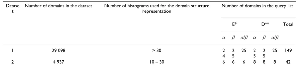
Table 1: The content of the datasets and the query lists used for PRIDE testing

Datase t

Number of domains in the dataset Number of histograms used for the domain structure representation

Number of domains in the query list

E* D** Total

α β α/β α β α/β

1 29 098 > 30 2

4 2 5

25 2 5

2 5

25 149

2 4 937 10 – 30 6 6 6 8 8 8 42

*E corresponds to the "easy" cases when the queries belong to highly populated groups of investigated datasets containing at least 50 domains at the homologous superfamily classification level of CATH;

tecture A (the number, type, and reciprocal orientation of the secondary structural elements), topology T (the topo-logical connection of the secondary structural elements) and homologous superfamily H (a common evolutionary origin supported either by significant sequence similarity or significant structural and functional similarity). Two datasets were created (Table 1), one with domains large enough to be represented by at least 30 distributions of Cαi-Cα(i+n) distances, and the other with smaller domains,

for which 10 < n_max < 30. Domains containing more then one polypeptide chain were disregarded since, by defini-tion, PRIDE cannot handle them.

Query lists

A non-redundant series of CATH entries were randomly selected from different superfamilies to be used as queries, by ensuring that all the three principal classes C of the database are equally represented (Table 1). Some were large domains (n_max > 30) and other small domains (10 <

nmax < 30). About half of them were considered to be

"easy" queries, in the sense that they belong to a CATH fold cluster containing at least 50 domains, and the others were "difficult" queries that belong to small CATH fold groups having no more than 3 domains.

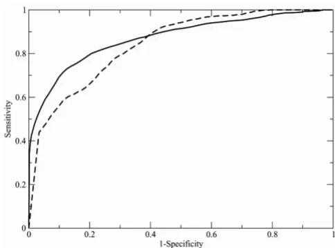
Performance evaluation

The performance of the new PRIDE version can be exam-ined by the computation and the analysis of the ROC curves. The P value, which is a similarity score, is used to calculate ROC curve in the present study. A threshold sim-ilarity is consecutively decreased, with subsequent decre-ments equal to 0.01, in the entire range of possible P values, from 1 to 0. At each step, each of the queries (Table 1) was compared to all the entries of the databases (Table 1). As a consequence, 4,335,602 comparisons were per-formed by considering the dataset of large protein domains and 207,354 comparisons were necessary by considering the dataset of small protein domains.

Each comparison can be classified in one of four catego-ries, according to the CATH classification of two domains and their P value. It can be i) a true positive (TP), if the similarity between the query and the entry is higher that the threshold value and if the query and the entry belong to the same CATH fold; ii) false positive (FP) if the simi-larity between the query and the entry is higher that the threshold value despite the fact that they have different CATH classification; iii) a false negative (FN), if the entry and the query are in the same fold cluster despite their estimated similarity is lower than the threshold value; iv) a true negative (TN), if the similarity is estimated to be smaller that the threshold value and if the query and the entry are actually classified into different CATH fold groups. On the basis of these definitions it is possible to

compute, for each threshold value, the sensitivity and the specificity

Sensitivity = TP/(TP + FN)

Specificity = TN/(TN + FP)

and the ROC curve is obtained by potting Sensitivity against (1-Specificity) for the entire range of possible threshold values. Figure 1 shows the ROC curves obtained as described above. It is necessary to remember that the line through the origin with slope 1, that is the diagonal, would correspond to the similarity detection based on a random measure. Therefore, the area under ROC curve equal to 0.5 is related to a random similarity measure, larger values indicate better than random estimations, and a value equal to 1 indicates perfect similarity. The areas under the ROC curves, shown in Figure 1, are 0.87 and 0.82 for the first and second datasets of Table 1, respec-tively. Not surprisingly, the area under the ROC curve is larger (0.87) for the first dataset of Table 1, which con-tains larger protein domains that can be described with at least 30 histograms of Cαi-Cα(i+n) distances, and smaller

(0.82) for the second dataset, which contains smaller pro-teins that are represented by a lower number of histo-grams. Such values are considerably better than that obtained by using the old version of PRIDE (0.55). These values are also comparable to those obtained with two other procedures for evaluating protein structure

similar-ROC curves

Figure 1

Publish with BioMed Central and every scientist can read your work free of charge "BioMed Central will be the most significant development for disseminating the results of biomedical researc h in our lifetime."

Sir Paul Nurse, Cancer Research UK

Your research papers will be:

available free of charge to the entire biomedical community

peer reviewed and published immediately upon acceptance

cited in PubMed and archived on PubMed Central

yours — you keep the copyright

Submit your manuscript here:

http://www.biomedcentral.com/info/publishing_adv.asp

BioMedcentral

ity – SHEBA (0.93) and VAST (0.90) that are computa-tionally much more demanding then the methods described in the present manuscript [18]. The areas under the ROC curves were also computed by using separately queries that are classified into the α, β, and α/β classes within the CATH database in order to estimate the per-formance of PRIDE on different types of proteins. Values of 0.90, 0.90, and 0.83 were obtained by scanning the database of 29,098 domains with the query sets contain-ing 49 α proteins, 50 β proteins, and 50 α/β proteins (dataset number 1 of Table 1), indicating that proteins containing both helices and strands are more difficult to be correctly identified, probably because of the higher structural diversity of protein domains containing differ-ent types of secondary structural elemdiffer-ents. Additional information is available at [21] (Downloads section).

Competing interests

The authors declare that they have no competing interests.

Authors' contributions

OC supervised and coordinated the project. SK developed the algorithm, carried out the analyses, and prepared, with OC, in the writing of the manuscript. All authors read and approved the manuscript.

Acknowledgements

This work was supported by the BIN-II network of the GEN-AU Austrian project.

References

1. Kolodny R, Petrey D, Honig B: Protein structure comparison: implications for the nature of 'fold space', and structure and function prediction. Curr Opin Struct Biol 2006, 16(3):393-398. 2. Carugo O: Rapid methods for comparing protein structures

and scanning structure databases. Curr Bioinformatics 2006,

1:75-83.

3. Carugo O: Recent progress in measuring structural similarity between proteins. Curr Protein Pept Sci 2007, 8:219-241. 4. Aung Z, Tan KL: Rapid retrieval of protein structures from

databases. Drug Disco Today 2007, in press:.

5. Pearson WR, Lipman DJ: Improved tools for biological sequence comparison. Proc Natl Acad Sci USA 1988, 85:2444-2448. 6. Altschul SF, Gish W, Miller W, Myers EW, Lipman DJ: Basil local

alignment search tool. J Mol Biol 1990, 215:403-410.

7. Altschul SF, Madden TL, Schaffer AA, Zhang J, Zhang Z, Miller W, Lip-man DJ: Gapped BLAST and PSI-BLAST: a new generation of protein database search programs. Nucl Acids Res 1997,

25:3389-3402.

8. Leinonen R, Diez FG, Binns D, Fleischmann W, Lopez R, Apweiler R:

UniProt archive. Bioinformatics 2004, 20:3226-3227.

9. Carugo O, Pongor S: Protein fold similarity estimated by a probabilistic approach based on C(alpha)-C(alpha) distance comparison. J Mol Biol 2002, 315(4):887-898.

10. Rogen P, Fain B: Automatic classification of protein structure by using Gauss integrals. Proc Natl Acad Sci USA 2003,

100:119-124.

11. Bostick DL, Shen M, Vaisman: A simple topological representa-tion of protein structure: implicarepresenta-tions for new, fast, and robust structural classification. Proteins 2004, 56(3):487-501. 12. Zotenko E, Dogan RI, Wilbur WJ, O'Leary DP, Przytycka TM:

Struc-tural footprinting in protein structure comparison: the impact of structural fragments. BMC Struct Biol 2007, 7:53.

13. Choi IG, Kwon J, Kim SH: Local feature frequency profile: a method to measure structural similarity in proteins. Proc Natl Acad Sci USA 2004, 101:3797-3802.

14. Frishman D, Argos P: Knowledge-based protein secondary structure assignment. Proteins 1995, 23:566-579.

15. Cruickshank DWJ: Coordinate uncertainty. In International Tables for CrystallographyVolume F. Edited by: Rossmann MG, Arnold E. Dor-drecht , Kluwer Academic Publisher; 2001:403-418.

16. Freedman D, Diaconis P: On the histogram as a density estima-tor: L2 theory. Probability Theory and Related Fields 1081,

57:453-476.

17. Dowdy S, Wearden S, Chilko D: Statistics for research. Hoboken , John Wiley & Sons; 2004.

18. Sam V, Tai CH, Garnier J, Gibrat JF, Lee B, Munson PJ: ROC and confusion analysis of structure comparison methods identify the main causes of divergence from manual protein classifi-cation. BMC Bioinformatics 2006, 7:206.

19. Novotny M, Madsen D, Kleywegt GJ: Evaluation of protein fold comparison servers. Proteins 2004, 54:260-270.

20. Orengo CA, Michie AD, Jones S, Jones DT, Swindells MB, Thornton JM: CATH--a hierarchical classification of protein domain structures. Structure 1997, 5:1093-1108.