Geometry with an Introduction to Cosmic Topology

(1)

Geometry

with an Introduction to

Cosmic Topology

2018 Edition

(2)

Department of Mathematics Lineld College

McMinnville, OR 97128 http://mphitchman.com

This work is licensed under the Creative Commons Attribution-ShareAlike 4.0 International License. To view a copy of this license, visit http:// creativecommons.org/licenses/by-sa/4.0/.

2018 Edition

ISBN-13: 978-1717134813 ISBN-10: 1717134815

A current version can always be found for free at http://mphitchman.com

(3)

Preface

Geometry with an Introduction to Cosmic Topology approaches geometry through the lens of questions that have ignited the imagination of stargazers since antiquity. What is the shape of the universe? Does the universe have an edge? Is it innitely big?

This text develops non-Euclidean geometry and geometry on surfaces at a level appropriate for undergraduate students who have completed a multivariable calculus course and are ready for a course in which to practice the habits of thought needed in advanced courses of the undergraduate mathematics curriculum. The text is also suited to independent study, with essays and discussions throughout.

Mathematicians and cosmologists have expended considerable amounts of eort investigating the shape of the universe, and this eld of research is called cosmic topology. Geometry plays a fundamental role in this research. Under basic assumptions about the nature of space, there is a simple relationship between the geometry of the universe and its shape, and there are just three possibilities for the type of geometry: hyperbolic geometry, elliptic geometry, and Euclidean geometry. These are the geometries we study in this text.

Chapters 2 through 7 contain the core mathematical content. The text follows the Erlangen Program, which develops geometry in terms of a space and a group of transformations of that space. Chapter 2 focuses on the complex plane, the space on which we build two-dimensional geometry. Chapter 3 details transformations of the plane, including Möbius transformations. This chapter marks the heart of the text, and the inversions in Section 3.2 mark the heart of the chapter. All non-Euclidean transformations in the text are built from inversions. We formally dene geometry in Chapter 4, and pursue hyperbolic and elliptc geometry in Chapters 5 and 6, respectively. Chapter 7 begins by extending these geometries to dierent curvature scales. Section 7.4 presents a unied family of geometries on all curvature scales, emphasizing key results common to them all. Section 7.5 provides an informal development of the topology of surfaces, and Section 7.6 relates the topology of surfaces to geometry, culminating with the Gauss-Bonnet formula. Section 7.7 discusses quotient spaces, and presents an important tool of cosmic topology, the Dirichlet domain.

Two longer essays bookend the core content. Chapter 1 introduces the geometric perspective taken in this text. In my experience it is very helpful to spend time discussing this content in class. The Coneland and Saddleland activities (Example 1.3.5 and Example 1.3.7) have proven particularly helpful for motivating the content of the text. In Chapter 8, after having developed two-dimensional non-Euclidean geometry and the topology of surfaces, we glance meaningfully at the present state of research in cosmic topology. Section 8.1 oers a brief survey of three-dimensional geometry and 3-manifolds, which

(4)

provide possible shapes of the universe. Sections 8.2 and 8.3 present two research programs in cosmic topology: cosmic crystallography and circles-in-the-sky. Measurements taken and analyzed over the last twenty years have greatly altered the way many cosmologists view the universe, and the text ends with a discussion of our present understanding of the state of the universe.

Compass and ruler constructions play a visible role in the text, primarily because inversions are emphasized as the basic building blocks of transfor-mations. Constructions are used in some proofs (such as the Fundamental Theorem of Möbius Transformations) and as a guide to denitions (such as the arc-length dierential in the hyperbolic plane). We encourage readers to practice constructions as they read along, either with compass and ruler on paper, or with software such as The Geometer's Sketchpad or Geogebra. Some Geometer's Sketchpad templates and activites related to the text can be found at the text's website.

Reading the text online An online text is fabulous at linking content, but we emphasize that this text is meant to be read. It was written to tell a mathematical story. It is not meant to be a collection of theorems and examples to be consulted as a reference. As such, online readers of this text are encouraged to turn the pages using the arrow buttons on the page as opposed to clicking on section links. Read the content slowly, participate in the examples, and work on the exercises. Grapple with the ideas, and ask questions. Feel free to email the author with questions or comments about the material.

Changes from the previously published version For those familiar with the oringial version of the text published by Jones & Bartlett, we note a few changes in the current edition. First, the numbering scheme has changed, so Example and Theorem and Figure numbers will not match the old hard copy. Of course the numbering schemes on the website and the new print options of the text do agree. Second, several exercises have been added. In sections with additional exercises, the new ones typically appear at the end of the section. Finally, Chapter 7 has been reorganized in an eort to place more emphasis on the family (Xk, Gk), and the key theorems common to all these

(5)

Acknowledgements

Many people helped with the development of this text. Je Weeks' text The Shape of Space inspired me to rst teach a geometry course motivated by cosmic topology. Colleagues at The College of Idaho encouraged me to teach the course repeatedly as the manuscript developed, and students there provided valuable feedback on how this story can be better told.

I would like to thank Rob Beezer, David Farmer, and all my colleagues at the UTMOST 2017 Textbook Workshop and in the PreTeXt Community for helping me convert my dusty tex code to a workable PreTeXt document in order to make the text freely available online, both as a webpage and as a printable document. I also thank Jennifer Nordstrom for encouraging me to use PreTeXt in the rst place.

I owe my colleagues at The College of Idaho and the University of Oregon a debt of gratitude for helping to facilitate a sabbatical during which an earlier incarnation of this text developed and was subsequently published in 2009 with Jones & Bartlett. Richard Koch discussed some of its content with me, and Jim Dull patiently discussed astrophysics and cosmology with me at a moment's notice.

The pursuit of detecting the shape of the universe has rapidly evolved over the last twenty years, and Marcelo Rebouças kindly answered my questions regarding the content of Chapter 8 back in 2008, and pointed me to the latest papers. I am also grateful to the authors of the many cosmology papers accessible to the amateur enthusiast and written with the intent to inform.

Finally, I would like to thank my family for their support during this endeavor, for letting this project permeate our home, and for encouraging its completion when we might have done something else, again.

(6)

(7)

(8)

(9)

An Invitation to Geometry

How can it be that mathematics, being after all a product of human thought which is independent of experience, is so admirably appropriate to the objects of reality?

Albert Einstein

Out of nothing I have created a strange new universe.

János Bolyai

1.1 Introduction

Imagine you are a two-dimensional being living in a two-dimensional universe. Mathematicians in this universe often represent its shape as an innite plane, exactly like thexy-plane you've used as the canvas in your calculus courses.

Your two-dimensional self has been taught in geometry that the angles of any triangle sum to 180◦_{. You may have even constructed some triangles to}

check. Builders use the Pythagorean theorem to check whether two walls meet at right angles, and houses are sturdy.

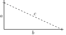
c a

[image:11.612.218.344.479.546.2]

b

Figure 1.1.1: Measurea,b, andcand check whethera2₊_b2₌_c2_{. If equality}

holds, the corner is square!

The innite plane model of the two-dimensional universe works well enough for most purposes, but cosmologists and mathematicians, who notice that everything within the universe is nite, consider the possibility that the universe itself is nite. Would a nite universe have a boundary? Can it have an edge, a point beyond which one cannot travel? This possibility is

(12)

unappealing because a boundary point would be physically dierent from the rest of space. But how can a nite universe have no boundary?

[image:12.612.281.388.441.498.2]

In a stroke as bold as it is simple, a two-dimensional mathematician suggests that the universe looks like a rectangular region with opposite edges identied. Consider a at, two-dimensional rectangle. In fact, visualize a tablet screen. Now imagine that you are playing a video game called Asteroids. As you shoot the asteroids and move your ship around the screen, you nd that if you go o the top of the screen your ship reappears on the bottom; and if you go o the screen to the left you reappear on the right. In Figure 1.1.2 there are just ve asteroids. One has partially moved o the top of the screen and reappeared below, while a second is half way o the right hand edge and is reappearing to the left.

Figure 1.1.2: A nite two-dimensional world with no boundary.

Thus, the top edge of the rectangle has been identied, point by point, with the bottom edge. In three dimensions one can physically achieve this identication, or gluing, of the edges. In particular, one can bend the rectangle to produce a cylinder, being careful to join only the top and bottom edges together, and not any other points. The left and right edges of the rectangle have now become the left and right circles of the cylinder, which themselves get identied, point by point. Bend the cylinder to achieve this second gluing, and one obtains a donut, also called a torus.

Figure 1.1.3: The video screen in Figure 1.1.2 is equivalent to a torus.

Of course your two-dimensional self would not be able to see this torus surface in 3-space, but you could understand the space perfectly well in its rectangle-with-edges-identied form. It is clearly a nite area universe without any edge.

A sphere, like the surface of a beach ball, is another nite area two-dimensional surface without any edge. A bug cruising around on the surface of a sphere will observe that locally the world looks like a at plane, and that the surface has no edges.

Consideration of a nite-area universe leads to questions about the type of geometry that applies to the universe. Let's look at a sphere. On small scales Euclidean geometry works well enough: small triangles have angle sum essentially equal to 180◦_{, which is a dening feature of Euclidean geometry.}

(13)

1.2. A Brief History of Geometry 3

mean three points on the surface, together with three paths of shortest distance between the points. We'll discuss this more carefully later.)

Consider the triangle formed by the north pole and two points on the equator in Figure 1.1.4. The angle at each point on the equator is 90◦_{, so the}

total angle sum of the triangle exceeds 180◦ _{by the amount of the angle at the}

north pole. We conclude that a non-Euclidean geometry applies to the sphere on a global scale.

Figure 1.1.4: A triangle on a sphere.

In fact, there is a wonderful relationship between the topology (shape) of a surface, and the type of geometry that it inherits, and a primary goal of this book is to arrive at this relationship, given by the pristine Gauss-Bonnet equation

kA= 2πχ.

We won't explain this equation here, but we will point out that geometry is on the left side of the equation, and topology is on the right. So, if a two-dimensional being can deduce what sort of global geometry holds in her world, she can greatly reduce the possible shapes for her universe. Our immediate task in the text is to study the other, non-Euclidean types of geometry that may apply on surfaces.

1.2 A Brief History of Geometry

Geometry is one of the oldest branches of mathematics, and most important among texts is Euclid's Elements. His text begins with 23 denitions, 5 postulates, and 5 common notions. From there Euclid starts proving results about geometry using a rigorous logical method, and many of us have been asked to do the same in high school.

Euclid's Elements served as the text on geometry for over 2000 years, and it has been admired as a brilliant work in logical reasoning. But one of Euclid's ve postulates was also the center of a hot debate. It was this debate that ultimately led to the non-Euclidean geometries that can be applied to dierent surfaces.

Here are Euclid's ve postulates:

1. One can draw a straight line from any point to any point.

2. One can produce a nite straight line continuously in a straight line. 3. One can describe a circle with any center and radius.

4. All right angles equal one another.

(14)

Does one postulate not look like the others? The rst four postulates are short, simple, and intuitive. Well, the second might seem a bit odd, but all Euclid is saying here is that you can produce a line segment to any length you want. However, the 5th one, called the parallel postulate, is not short or simple; it sounds more like something you would try to prove than something you would take as given.

Indeed, the parallel postulate immediately gave philosophers and other thinkers ts, and many tried to prove that the fth postulate followed from the rst four, to no avail. Euclid himself may have been bothered at some level by the parallel postulate since he avoids using it until the proof of the 29th proposition in his text.

In trying to make sense of the parallel postulate, many equivalent statements emerged. The two equivalent statements most relevant to our study are these:

50_{. Given a line and a point not on the line, there is exactly one}

line through the point that does not intersect the given line.

500. The sum of the angles of any triangle is 180◦.

Reformulation50 of the parallel postulate is called Playfair's Axiom after the

Scottish mathematician John Playfair (1748-1819). This version of the fth postulate will be the one we alter in order to produce non-Euclidean geometry. The parallel postulate debate came to a head in the early 19th century. Farkas Bolyai (1775-1856) of Hungary spent much of his life on the problem of trying to prove the parallel postulate from the other four. He failed, and he fretted when his son János (1802-1860) started following down the same tormented path. In an oft-quoted letter, the father begged the son to end the obsession:

For God's sake, I beseech you, give it up. Fear it no less than the sensual passions because it too may take all your time and deprive you of your health, peace of mind and happiness in life.1

But János continued to work on the problem, as did the Russian mathematician Nikolai Lobachevsky (1792-1856). They independently discovered that a well-dened geometry is possible in which the rst four postulates hold, but the fth doesn't. In particular, they demonstrated that the fth postulate is not a necessary consequence of the rst four.

In this text we will study two types of non-Euclidean geometry. The rst type is called hyperbolic geometry, and is the geometry that Bolyai and Lobachevsky discovered. (The great Carl Friedrich Gauss (1777-1855) had also discovered this geometry; however, he did not publish his work because he feared it would be too controversial for the establishment.) In hyperbolic geometry, Euclid's fth postulate is replaced by this:

5H. Given a line and a point not on the line, there are at least two lines through the point that do not intersect the given line.

In hyperbolic geometry, the sum of the angles of any triangle is less than 180◦_,

a fact we prove in Chapter 5.

The second type of non-Euclidean geometry in this text is called elliptic geometry, which models geometry on the sphere. In this geometry, Euclid's fth postulate is replaced by this:

1_{See for instance, Martin Gardner's book The Colossal Book of Mathematics, W.W.}

(15)

1.2. A Brief History of Geometry 5

5E. Given a line and a point not on the line, there are zero lines through the point that do not intersect the given line.

In elliptic geometry, the sum of the angles of any triangle is greater than 180◦_,

a fact we prove in Chapter 6.

The Pythagorean Theorem The celebrated Pythagorean theorem depends upon the parallel postulate, so it is a theorem of Euclidean geometry. However, we will encounter non-Euclidean variations of this theorem in Chapters 5 and 6, and present a unied Pythagorean theorem in Chapter 7, with Theorem 7.4.7, a result that appeared recently in [20].

The Pythagorean theorem appears as Proposition 47 at the end of Book I of Euclid's Elements, and we present Euclid's proof below. The Pythagorean theorem is fundamental to the systems of measurement we utilize in this text, in both Euclidean and non-Eucidean geometries. We also remark that the nal proposition of Book I, Proposition 48, gives the converse that builders use: If we measure the legs of a triangle and nd that c2 ₌_a2₊_b2 _{then the angle}

oppositecis right. The interested reader can nd an online version of Euclid's Elements here [29].

Theorem 1.2.1 The Pythagorean Theorem. In right-angled triangles the square on the side opposite the right angle equals the sum of the squares on the sides containing the right angle.

Proof. Suppose we have right triangle ABC as in Figure 1.2.2 with right angle at C, and side lengthsa, b, and c, opposite corners A, B and C, respectively. In the gure we have extended squares from each leg of the triangle, and labeled various corners. We have also constructed the line through Cparallel toAD, and letLandM denote the points of intersection of this line with AB and DE, respectively. One can check that ∆KAB is congruent to

∆CAD. Moreover, the area of∆KAB is one half the area of the squareAH. This is the case because they have equal base (segmentKA) and equal altitude (segmentAC). By a similar argument, the area of∆DACis one half the area of the parallelogramAM. This means that squareAHand parallelogramAM have equal areas, the value of which isb2.

One may proceed as above to argue that the areas of square BG and parallelogram BM are also equal, with value a2. Since the area of square BD, which equalsc2, is the sum of the two parallelogram areas, it follows that a2₊_b2₌_c2_.

The arrival of non-Euclidean geometry soon caused a stir in circles outside the mathematics community. Fyodor Dostoevsky thought non-Euclidean geometry was interesting enough to include in The Brothers Karamazov, rst published in 1880. Early in the novel two of the brothers, Ivan and Alyosha, get reacquainted at a tavern. Ivan discourages his younger brother from thinking about whether God exists, arguing that if one cannot fathom non-Euclidean geometry, then one has no hope of understanding questions about God.2

One of the rst challenges of non-Euclidean geometry was to determine its logical consistency. By changing Euclid's parallel postulate, was a system created that led to contradictory theorems? In 1868, the Italian mathematician Enrico Beltrami (1835-1900) showed that the new non-Euclidean geometry could be constructed within the Euclidean plane so that, as long as Euclidean 2_{See, for instance, The Brothers Karamazov, Fyodor Dostoevsky (a new translation by}

(16)

B

E L

M

F

A

D K

H

C G

Figure 1.2.2: Proving the Pythagorean theorem

geometry was consistent, non-Euclidean geometry would be consistent as well. Non-Euclidean geometry was thus placed on solid ground.

This text does not develop geometry as Euclid, Lobachevsky, and Bolyai did. Instead, we will approach the subject as the German mathematician Felix Klein (1849-1925) did.

Whereas Euclid's approach to geometry was additive (he started with basic denitions and axioms and proceeded to build a sequence of results depending on previous ones), Klein's approach was subtractive. He started with a space and a group of allowable transformations of that space. He then threw out all concepts that did not remain unchanged under these transformations. Geometry, to Klein, is the study of objects and functions that remain unchanged under allowable transformations.

Klein's approach to geometry, called the Erlangen Program after the university at which he worked at the time, has the benet that all three geometries (Euclidean, hyperbolic and elliptic) emerge as special cases from a general space and a general set of transformations.

The next three chapters will be devoted to making sense of and working through the preceding two paragraphs.

Like so much of mathematics, the development of non-Euclidean geom-etry anticipated applications. Albert Einstein's theory of special relativity illustrates the power of Klein's approach to geometry. Special relativity, says Einstein, is derived from the notion that the laws of nature are invariant with respect to Lorentz transformations.3

Even with non-Euclidean geometry in hand, Euclidean geometry remains central to modern mathematics because it is an excellent model for our local geometry. The angles of a triangle drawn on this paper do add up to 180◦_.

Even galactic triangles determined by the positions of three nearby stars have angle sum indistinguishable from 180◦_.

However, on a larger scale, things might be dierent.

Maybe we live in a universe that looks at (i.e., Euclidean) on smallish scales but is curved globally. This is not so hard to believe. A bug living in a eld on the surface of the Earth might reasonably conclude he is living on an innite plane. The bug cannot sense the fact that his at, visible world is just a small patch of a curved surface (Earth) living in three-dimensional space. Likewise, our apparently Euclidean three-dimensional universe might

(17)

1.3. Geometry on Surfaces: A First Look 7

be curving in some unseen fourth dimension so that the global geometry of the universe might be non-Euclidean.

Under reasonable assumptions about space, hyperbolic, elliptic, and Euclidean geometry are the only three possibilities for the global geometry of our universe. Researchers have spent signicant time poring over cosmological data in hopes of deciding which geometry is ours. Deducing the geometry of the universe can tell us much about the shape of the universe and perhaps whether it is nite. If the universe is elliptic, then it must be nite in volume. If it is Euclidean or hyperbolic, then it can be either nite or innite. Moreover, each geometry type corresponds to a class of possible shapes. And, if that isn't exciting enough, the overall geometry of the universe may be fundamentally connected to the fate of the universe. Clearly there is no more grand application of geometry than to the fate of the universe!

Exercises

1. Use Euclid's parallel postulate to prove the alternate interior angles theorem. That is, in Figure 1.2.3(a), assume the lineBD is parallel to the line AC. Prove that_∠BAC=_∠ABD.

2. Use Euclid's parallel postulate and the previous problem to prove that the sum of the angles of any triangle is 180◦_{. You may nd Figure 1.2.3(b)}

helpful, where segmentCD is parallel to segmentAB.

A

B

C D

(a) A

B

C D

(b)

Figure 1.2.3: Two consequences of the parallel postulate.

1.3 Geometry on Surfaces: A First Look

Think for a minute about the space we live in. Think about objects that live in our space. Do the features of objects change when they move around in our space? If I pick up this paper and move it across the room, will it shrink? Will it become a broom?

If you draw a triangle on this page, the angles of the triangle will add to 180◦_{. In fact, any triangle drawn anywhere on the page has this property.}

Euclidean geometry on this at page (a portion of the plane) is homogeneous: the local geometry of the plane is the same at all points. Our three-dimensional space appears to be homogeneous as well. This is nice, for it means that if we buy a 5 ft3_{freezer at the appliance store, it doesn't shrink to 0.5 ft}3 _{when we}

get it home. A sphere is another example of a homogenous surface. A two-dimensional bug living on the surface of a sphere could not tell the dierence (geometrically) between any two points on the sphere.

(18)

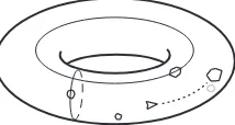
Figure 1.3.1: This torus surface is not homogeneous.

It is an important matter to decide what we mean, exactly, by a triangle on a surface. A triangle consists of three points and three edges connecting these points. An edge connecting pointA to pointB is drawn to represent the path of shortest distance betweenA andB. Such a path is called a geodesic. For the two-dimensional bug, a straight line fromA toB is simply the shortest path fromAto B.

On a sphere, geodesics follow great circles. A great circle is a circle drawn on the surface of the sphere whose center (in three-dimensional space) corresponds to the center of the sphere. Put another way, a great circle is a circle of maximum diameter drawn on the sphere. The circles a and b in Figure 1.3.2 are great circles, but circlec is not.

a

b

c

Figure 1.3.2: Geodesics on the sphere are great circles.

In the Euclidean plane, geodesics are Euclidean lines. One way to determine a geodesic on a surface physically is to pin some string atAand draw the string tight on the surface to a pointB. The taut string will follow the geodesic from A to B. In Figure 1.3.3 we have drawn geodesic triangles on three dierent surfaces.

Figure 1.3.3: Depending on the shape of the surface, geodesic triangles can have angle sum greater than, less than, or equal to 180◦_.

(19)

She'd go home, write up the result, emphasizing the fact that a triangle in the rst convex region will have angle sum greater than 180◦_{, while a triangle}

in the saddle-shaped region will have angle sum less than 180◦_{. This happy}

bug will conclude her donut surface is not homogeneous. She will then sit back and watch the accolades pour in. Perhaps even a Nobel prize. Thus, small triangles and their angles can help a two-dimensional bug distinguish points on a surface.

The donut surface is not homogeneous, so let's build one that is. Example 1.3.4: The Flat Torus.

Consider again the world of Figure 1.1.2. This world is called a at torus. At every spot in this world, the pilot of the ship would report at surroundings (triangle angles add to 180◦_{). Unlike the donut surface}

living in three dimensions, the at torus is homogeneous. Locally, geometry is the same at every point, and thanks to a triangle check, this geometry is Euclidean. But the world as a whole is much dierent than the Euclidean plane. For instance, if the pilot of the ship has a powerful enough telescope, he'd be able to see the back of his ship. Of course, if the ship had windows just so, he'd be able to see the back of his head. The at torus is a nite, Euclidean two-dimensional world without any boundary.

Example 1.3.6: Coneland.

Here we build cones from at wedges, and measure angles of some triangles.

a. Begin with a circular disk with a wedge removed, like a pizza missing a slice or two. Joining the two radial edges produces a cone. Try it with a cone of your own to make sure it works. Now, with the cone at again, pick three points, labeled A,B, andC, such that C is on the radial edge. This means that in this attened version of the cone, pointC actually appears twice: once on each radial edge, as in Figure 1.3.6. These two representatives for C should get identied when you join the radial edges.

C C A

B

θ

Figure 1.3.6: A triangle on a cone.

(20)

don't get the tip of the cone on the inside of the triangle, adjust the points accordingly.

c. With your protractor, carefully measure the angleθ subtended by the circular sector. To emphasize θ's role in the shape of the cone, we letS(θ)denote the cone surface determined byθ.

d. With your protractor, carefully measure the three angles of your triangle. The angle at point C is the sum of the angles formed by the triangle legs and the radial segments. Let∆ denote the sum of these

three angles.

e. State a conjecture about the relationship between the angle θ and ∆, the sum of the angles of the triangle. Your conjecture can be

in the form of an equation. Then prove your conjecture. Hint: if you draw a segment connecting the 2 copies of point C, what is the angle sum of the quadrilateralABCC?

Example 1.3.7: Saddleland.

Repeat the previous exercise but with circle wedges having θ > 2π. Identifying the radial edges in this case produces a saddle-shaped surface. [To create such a circle wedge we can tape together two wedges of equal radius. One idea: Start with a disk with one radial cut, and a wedge of equal radius. Tape one radial edge of the wedge to one of the slit radial edges of the disk. Then, identifying the other radial edges should produce Saddleland.]

Remember, a homogeneous surface is a space that has the same local geometry at every point. Our at torus is homogeneous, having Euclidean geometry at every point. However, our cones S(θ) in the previous exercises

are not homogeneous (unlessθ happens to be 2π). If a triangle in S(θ)does

not contain the tip of the cone in its interior, then the angles of the triangle will add to π radians, but if the triangle does contain the tip of the cone in its interior, then the angle sum will not beπradians. A two-dimensional bug, then, could conclude thatS(θ)is not homogeneous.

c a

b

c

a

b H

Figure 1.3.8: A hexagonal video screen

Example 1.3.9: A non-Euclidean surface.

(21)

hexagonal screen at a spot on the edge markeda, say, then it reappears at the matching spot on the other edge markeda.

Suppose the pilot of a ship wants to y around one of the corners of the hexagon. If she begins at point H, say, and ies counterclockwise around the upper right corner as indicated in the diagram, she would y o the screen at the top near the start of an a edge. So, as she made her journey, she would reappear in the lower left corner near the start of the other aedge. Continuing around she would complete her journey after circling this second corner.

However, the angle of each corner is 120◦_{, and gluing them together}

will create a cone point, as pictured below. Similarly, she would nd that the other corners of the hexagon meet in groups of two, creating two additional cone points. As with the Coneland Example 1.3.5, the pilot can distinguish a corner point from an interior point here. She can look at triangles: a triangle containing one of the cone points will have angle sum greater than 180◦_{; any other triangle will have angle}

sum equal to 180◦_.

a

c

H

So the surface is not homogeneous, if it is drawn in the plane. However, the surface does admit a homogeneous geometry. We can get rid of the cone points if we can increase each corner angle of the hexagon to 180◦_{. Then, two corners would come together to form a}

perfect 360◦ _{patch about the point.}

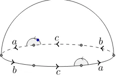
But how can we increase the corner angles? Put the hexagon on the sphere! Imagine stretching the hexagon onto the northern hemisphere of a sphere (see Figure 1.3.10). In this case we can think of the 6 points of our hexagon as lying on the equator. Then each corner angle is 180◦_{, each edge is still a line (geodesic), and when we glue}

the edges, each pair of corner angles adds up to exactly 360◦_{, so the}

surface is homogeneous. The homogeneous geometry of this surface is the geometry of the sphere (elliptic geometry), not the geometry of the plane (Euclidean geometry).

b

a c

c a

[image:21.612.219.336.558.635.2]

b

Figure 1.3.10: A surface with homogeneous elliptic geometry.

(22)

If it doesn't make a whole lot of sense right now, don't sweat it, but please use these facts as motivation for learning about these non-Euclidean geometries.

Exercises 1. Work through the Coneland Example 1.3.5. 2. Work through the Saddleland Example 1.3.7.

3. Circumference vs Radius in Coneland and Saddleland. In addition to triangles, a two-dimensional bug can use circles to screen for dierent geometries. In particular, a bug can study the relationship between the radius and the circumference of a circle. To make sure we think like the bug, here's how we dene a circle on a surface: Given a pointP on the surface, and a real number r >0, the circle centered atP with radius ris the set of all points r units away fromP, where the distance between two points is the length of the shortest path connecting them (the geodesic).

a. Pick your favorite circle in the plane. What is the relationship between the circle's radius and circumference? Is your answer true for any circle in the plane?

b. Consider the Coneland surface of Example 1.3.5. Construct a circle centered at the tip of the cone and derive a relationship between its circumference and its radius. IsC= 2πrhere? If not, which is true: C >2πr orC <2πr?

(23)

2

The Complex Plane

To study geometry using Klein's Erlangen Program, we need to dene a space and a group of transformations of the space. Our space will be the complex plane.

2.1 Basic Notions

The set of complex numbers is obtained algebraically by adjoining the number ito the set_Rof real numbers, whereiis dened by the property thati2₌₋₁_.

We will take a geometric approach and dene a complex number to be an ordered pair (x, y) of real numbers. We let _C denote the set of all complex

numbers,

C={(x, y)| x, y∈R}.

Given the complex numberz= (x, y),xis called the real part ofz, denoted Re(z); and y is called the imaginary part of z, denoted Im(z). The set of

real numbers is a subset ofCunder the identicationx↔(x,0), for any real

numberx.

Addition in Cis componentwise,

(x, y) + (s, t) = (x+s, y+t),

and ifkis a real number, we dene scalar multiplication by

k·(x, y) = (kx, ky).

Within this framework,i= (0,1), meaning that any complex number(x, y)

can be expressed asx+yias suggested here:

(x, y) = (x,0) + (0, y)

=x(1,0) +y(0,1)

=x+yi.

The expressionx+yiis called the Cartesian form of the complex number. This form can be helpful when doing arithmetic of complex numbers, but it can also be a bit gangly. We often let a single letter such aszorwrepresent a complex number. So,z=x+yimeans that the complex number we're calling z corresponds to the point(x, y)in the plane.

It is sometimes helpful to view a complex number as a vector, and complex addition corresponds to vector addition in the plane. The same holds for scalar multiplication. For instance, in Figure 2.1.1 we have represented z = 2 +i, w=−1 + 1.5i, as well asz+w= 1 + 2.5i, as vectors from the origin to these

(24)

points inC. The complex numberz−wcan be represented by the vector from

wtoz in the plane.

z w

z+w

i

1

z

w z−w

Figure 2.1.1: Complex numbers as vectors in the plane.

We dene complex multiplication using the fact thati2₌₋₁_.

(x+yi)·(s+ti) =xs+ysi+xti+yti2

= (xs−yt) + (ys+xt)i.

The modulus ofz=x+yi, denoted|z|, is given by

|z|=px2₊_y2_.

Note that |z|gives the Euclidean distance ofz to the point (0,0). The conjugate ofz=x+yi, denotedz, is

z=x−yi.

In the exercises the reader is asked to prove various useful properties of the modulus and conjugate.

Example 2.1.2: Arithmetic of complex numbers. Supposez= 3−4i andw= 2 + 7i.

Thenz+w= 5 + 3i, and

z·w= (3−4i)(2 + 7i)

= 6 + 28−8i+ 21i

= 34 + 13i.

A few other computations:

4z= 12−16i

|z|=p32_{+ (}₋₄₎2_{= 5}

zw= 34−13i.

Exercises

1. In each case, determinez+w,sz,|z|, andz·w. a. z= 5 + 2i,s=−4,w=−1 + 2i.

b. z= 3i,s= 1/2,w=−3 + 2i. c. z= 1 +i,s= 0.6,w= 1−i.

(25)

2.2. Polar Form of a Complex Number 15

3. Supposez=x+yiandw=s+tiare two complex numbers. Prove the following properties of the conjugate and the modulus.

a. |w·z|=|w| · |z|. b. zw=z·w. c. z+w=z+w.

d. z+z= 2Re(z). (Hence,z+z is a real number.) e. z−z= 2Im(z)i.

f. |z|=|z|.

4. A Pythagorean triple consists of three integers (a, b, c) such that

a2₊_b2 ₌_c2_{. We can use complex numbers to generate Pythagorean triples.}

Supposez=x+yiwherexandy are positive integers. Let

a=Re(z2) b=Im(z2) c=zz.

a. Prove thata2₊_b2₌_c2_.

b. Find the complex number z =x+yi that generates the famous triple (3,4,5).

c. Find the complex number that generates the triple (5,12,13).

d. Find ve other Pythagorean triples, generated using complex numbers of the form z=x+yi, wherexand y are positive integers with no common divisors.

2.2 Polar Form of a Complex Number

A point(x, y)in the plane can be represented in polar form(r, θ)according to

the relationships in Figure 2.2.1.

(x, y)

r

θ

x=rcos(θ)

y=rsin(θ)

Figure 2.2.1: Polar coordinates of a point in the plane

Using these relationships, we can rewrite

x+yi=rcos(θ) +rsin(θ)i

=r(cos(θ) +isin(θ)).

This leads us to make the following denition. For any real number θ, we dene

eiθ= cos(θ) +isin(θ).

For instance, eiπ/2= cos(π/2) +isin(π/2) = 0 +i·1 =i.

Similarly, ei0 _{= cos(0) +}_i_{sin(0) = 1}_{, and it's a quick check to see that}

eiπ₌₋₁_{, which leads to a simple equation involving the most famous numbers}

in mathematics (except 8), truly an all-star equation:

eiπ+ 1 = 0.

If z = x+yi and (x, y) has polar form (r, θ) then z = reiθ _{is called the}

(26)

Example 2.2.2: Exploring the polar form.

On the left side of the following diagram, we plot the points z = 2eiπ/4_{, w}_{= 3}_eiπ/2_{, v}₌₋₂_eiπ/6_{, u}_{= 3}_e−iπ/3_.

w

z

v

u

θ α

−3 + 4i

4

3

r

To convert z = −3 + 4i to polar form, refer to the right side of the diagram. We note that r =√9 + 16 = 5, andtan(α) = 4/3, so

θ=π−tan−1(4/3)≈2.21radians. Thus,

−3 + 4i= 5ei(π−tan−1(4/3))≈5e2.21i.

Theorem 2.2.3. The product of two complex numbers in polar form is given by

reiθ·seiβ= (rs)ei(θ+β).

Proof. We use the denition of the complex exponential and some trigonometric identities.

reiθ·seiβ=r(cosθ+isinθ)·s(cosβ+isinβ)

= (rs)(cosθ+isinθ)·(cosβ+isinβ)

=rs[cosθcosβ−sinθsinβ+ (cosθsinβ+ sinθcosβ)i]

=rs[cos(θ+β) + sin(θ+β)i]

=rs[ei(θ+β)].

Thus, the product of two complex numbers is obtained by multiplying their magnitudes and adding their arguments, and

arg(zw) = arg(z) + arg(w),

where the equation is taken modulo 2π. That is, depending on our choices for the arguments, we havearg(vw) = arg(v) + arg(w) + 2πkfor some integer k.

Example 2.2.4: Polar form with r≥0.

When representing a complex number z in polar form asz =reiθ_{, we}

may assume that ris non-negative. Ifr <0, then

reiθ=−|r|eiθ

= (eiπ)· |r|eiθ since −1 =eiπ

(27)

2.3. Division and Angle Measure 17

Thus, by addingπto the angle if necessary, we may always assume that z=reiθ _where_r_{is non-negative.}

Exercises

1. Convert the following points to polar form and plot them: 3 +i,−1−2i,

3−4i,7,002,001, and−4i.

2. Express the following points in Cartesian form and plot them: z= 2eiπ/3_,

w=−2eiπ/4_, _u_{= 4}_ei5π/3_,_and_z_·_u_.

3. Modify the all-star equation to involve 8. In particular, write an expression involving e, i, π,1, and 8, that equals 0. You may use no other numbers, and certainly not 3.

4. Ifz=reiθ_{, prove that}_z₌_re−iθ_.

2.3 Division and Angle Measure

The division of the complex numberz byw6= 0, denoted z

w, is the complex

numberuthat satises the equationz=w·u. For instance, 1

i =−ibecause1 =i·(−i).

In practice, division of complex numbers is not a guessing game, but can be done by multiplying the top and bottom of the quotient by the conjugate of the bottom expression.

Example 2.3.1: Division in Cartesian form. We convert the following quotient to Cartesian form:

2 +i

3 + 2i =

2 +i

3 + 2i·

3−2i

= (6 + 2) + (−4 + 3)i 9 + 4

= 8−i 13

= 8 13−

1 13i.

Example 2.3.2: Division in polar form.

Suppose we wish to nd z/w where z=reiθ andw =seiβ 6= 0. The

reader can check that

1

w =

1

se

−iβ_.

Then we may apply Theorem 2.2.3 to obtain the following result:

z w =z·

1

w

=reiθ· 1 se

−iβ

= r

se

(28)

So,

arg

_z

w

= arg(z)−arg(w)

where equality is taken modulo2π.

Thus, when dividing by complex numbers, we can rst convert to polar form if it is convenient. For instance,

1 +i −3 + 3i =

√ 2eiπ/4 √

18ei3π/4 =

1 3e

−iπ/2₌₋1

3i.

Angle Measure Given two raysL1andL2having common initial point, we

let∠(L1, L2)denote the angle between rays L1 andL2, measured fromL1

toL2. We may rotate rayL1onto rayL2in either a counterclockwise direction

or a clockwise direction. We adopt the convention that angles measured counterclockwise are positive, and angles measured clockwise are negative, and admit that angles are only well-dened up to multiples of2π. Notice that

∠(L1, L2) =−∠(L2, L1).

To compute∠(L1, L2)wherez0is the common initial point of the rays, let

z1 be any point onL1, andz2 any point onL2. Then

∠(L1, L2) = arg

_z

2−z0

z1−z0

= arg(z2−z0)−arg(z1−z0).

Example 2.3.3: The angle between two rays.

SupposeL1 andL2 are rays emanating from2 + 2i. RayL1 proceeds

along the liney=xandL2 proceeds alongy= 3−x/2as pictured.

L

₁

L

2

θ

2 + 2

i

3 + 3

i

4 +

i

To compute the angleθin the diagram, we choosez1= 3 + 3iand

z2= 4 +i. Then

∠(L1, L2) = arg(2−i)−arg(1 +i) =−tan−1(1/2)−π/4≈ −71.6◦.

That is, the angle fromL1toL2is 71.6◦in the clockwise direction.

The angle determined by three points.

If u, v, and ware three complex numbers, let _∠uvw denote the angle θ from ray−vu→to−vw→. In particular,

∠uvw=θ= arg

_w₋_v

u−v

(29)

2.4. Complex Expressions 19

θ

u

v

w

For instance, ifu= 1on the positive real axis,v= 0is the origin in_C, and

z is any point in_C, then_∠uvz= arg(z).

Exercises 1. Express 1

x+yi in the forma+bi.

2. Express these fractions in Cartesian form or polar form, whichever seems more convenient.

1 2i,

1 1 +i,

4 +i

1−2i,

2 3 +i.

3. Prove that|z/w|=|z|/|w|, and thatz/w=z/w.

4. Supposez=reiθ _and_w₌_seiα_{are as shown below. Let}_u₌_z_·_w_{. Prove}

that∆01zand∆0wuare similar triangles.

0 1

z w u

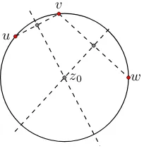
5. Determine the angle∠uvwwhereu= 2 +i,v= 1 + 2i, and w=−1 +i. 6. Supposezis a point with positive imaginary component on the unit circle shown below, a= 1 andb = −1. Use the angle formula to prove that angle ∠bza=π/2.

0 b

z

a

2.4 Complex Expressions

(30)

Example 2.4.1: Line equations.

The standard form for the equation of a line in the xy-plane is ax+by+d= 0. This line may be expressed via the complex variable

z=x+yi. For an arbitrary complex numberβ =s+ti, note that

βz+βz=

(sx−ty) + (sy+tx)i

+

(sx−ty)−(sy+tx)i

= 2sx−2ty.

It follows that the lineax+by+d= 0 can be represented by the

equation

αz+αz+d= 0 (equation of a line)

whereα= 1₂(a−bi)is a complex constant anddis a real number. Conversely, for any complex number α and real number d, the equation

αz+αz+d= 0

determines a line inC.

We may also view any line inCas the collection of points equidistant from

two given points.

Theorem 2.4.2. Any line inCcan be expressed by the equation|z−γ|=|z−β|

for suitably chosen pointsγ andβ in _C, and the set of all points (Euclidean) equidistant from distinct pointsγ andβ forms a line.

Proof. Given two points γ and β in C, z is equidistant from both if and

only if|z−γ|2₌_|_z₋_β_|2_{. Expanding this equation, we obtain}

(z−γ)(z−γ) = (z−β)(z−β)

|z|2−γz−γz+|γ|2=|z|2−βz−βz+|β|2

(β−γ)z+ (β−γ)z+ (|γ|2_{− |}_β_|2_{) = 0}_.

This last equation has the form of a line, letting α = (β−γ) and

d=|γ|2_{− |}_β_|2_.

Conversely, starting with a line we can nd complex numbersγandβ that do the trick. In particular, if the given line is the perpendicular bisector of the segmentγβ, then|z−γ|=|z−β| describes the line. We leave the details to the reader.

Example 2.4.3: Quadratic equations.

Supposez0 is a complex constant and consider the equationz2 =z0.

A complex numberzthat satises this equation will be called a square root ofz0, and will be written as

√ z0.

If we viewz0 =r0eiθ0 in polar form withr0 ≥0, then a complex

number z=reiθ _{satises the equation}_z2₌_z

0 if and only if

(31)

In other words, z satises the equation if and only if r2 ₌_r

0 and

2θ=θ0 (modulo2π).

As long as r0 is greater than zero, we have two solutions to the

equation, so thatz0 has two square roots:

±√r0eiθ0/2.

For instance, z2 = i has two solutions. Since i = 1eiπ/2, √i = ±eiπ/4. In Cartesian form,√i=±(

√ 2

2 +

√ 2 2 i).

More generally, the complex quadratic equationαz2₊_βz₊_γ_{= 0}

where α, β, γ are complex constants, will have one or two solutions. This marks an important dierence from the real case, where a quadratic equation might not have any real solutions. In both cases we may use the quadratic formula to hunt for roots, and in the complex case we have solutions

z= −β±

p

β2₋₄_αγ

2α .

For instance,z2_{+ 2}_z_{+ 4 = 0}_{has two solutions:}

z= −2± √

−12

2 =−1± √

3i

since√−1 =i.

Example 2.4.4: Solving a quadratic equation.

Consider the equationz2−(3 + 3i)z= 2−3i. To solve this equation forz we rst rewrite it as

z2−(3 + 3i)z−(2−3i) = 0.

We use the quadratic formula with α = 1, β = −(3 + 3i), and

γ=−(2−3i), to obtain the solution(s)

z=3 + 3i±

p

(3 + 3i)2_{+ 4(2}₋₃_i₎

2

z=3 + 3i± √

8 + 6i

2 .

To determine the solutions in Cartesian form, we need to evaluate √

8 + 6i. We oer two approaches. The rst approach considers the following task: Setx+yi=√8 + 6i and solve forxandy directly by squaring both sides to obtain a system of equations.

x+yi=√8 + 6i

(x+yi)2= 8 + 6i

x2−y2+ 2xyi= 8 + 6i.

Thus, we have two equations and two unknowns:

x2−y2= 8 (1)

(32)

In fact, we also know that x2₊_y2 ₌ _|_x₊_yi_|2 ₌ _|₍_x₊_yi₎2_| ₌

|8 + 6i|= 10, giving us a third equation

x2+y2= 10. (3)

Adding equations (1) and (3) yieldsx2= 9sox=±3. Substituting

x= 3into equation (2) yieldsy = 1; substitutingx=−3into (2) yields

y=−1. Thus we have two solutions: √

8 + 6i=±(3 +i).

We may also use the polar form to determine √8 + 6i. Consider the right triangle determined by the point 8 + 6i = 10eiθ _{pictured in}

the following diagram.

10

8 + 6i

θ

We know√8 + 6i=±√10eiθ/2_{, so we want to nd} _θ/₂_{. Well, we}

can determinetan(θ/2)easily enough using the half-angle formula

tan(θ/2) = sin(θ) 1 + cos(θ).

The right triangle in the diagram shows us that sin(θ) = 3/5 and cos(θ) = 4/5, sotan(θ/2) = 1/3. This means that any pointreiθ/2_lives

on the line through the origin having slope 1/3, and can be described by k(3 +i) for some scalar k. Since √8 + 6i has this form, it follows that √8 + 6i=k(3 +i)for somek. Since|√8 + 6i|=√10, it follows

that |k(3 +i)|=√10, sok=±1. In other words,√8 + 6i=±(3 +i).

Now let's return to the solution of the original quadratic equation in this example:

z=3 + 3i± √

8 + 6i

2

z=3 + 3i±(3 +i)

2 .

Thus,z= 3 + 2ior z=i.

Example 2.4.5: Circle equations.

If we letz=x+yiandz0=h+ki, then the complex equation

|z−z0|=r (equation of a circle)

describes the circle in the plane centered atz0 with radiusr >0.

To see this, note that

|z−z0|=|(x−h) + (y−k)i|

(33)

So|z−z0|=ris equivalent to the equation(x−h)2+ (y−k)2=r2

of the circle centered at z0with radiusr.

For instance,|z−3−2i|= 3describes the set of all points that are

3 units away from 3 + 2i. All suchz form a circle of radius 3 in the plane, centered at the point (3,2).

Example 2.4.6: Complex expressions as regions.

Describe each complex expression below as a region in the plane. 1. |1/z|>2.

Taking the reciprocal of both sides, we have|z|<1/2, which is

the interior of the circle centered at 0 with radius1/2.

2. Im(z)<Re(z).

Setz=x+yiin which case the inequality becomesy < x. This inequality describes all points in the plane under the liney =x, as pictured below.

3. Im(z) =|z|.

Settingz=x+yi, this equation is equivalent toy=py2₊_x2_.

Squaring both sides we obtain 0 = x2, so that x = 0. It

follows thaty =py2 ₌_|_y_| _{so the equation describes the points}

(0, y) withy ≥0. These points determine a ray on the positive

imaginary axis.

1 2

Im(z)<Re(z)

Im(z) =|z|

Moving forward, lines and circles will be especially important objects for us, so we end the section with a summary of their descriptions in the complex plane.

Lines and circles in C.

Lines and circles in the plane can be expressed with a complex variable z=x+yi.

The line ax+by+d = 0 in the plane can be represented by the

equation

αz+αz+d= 0

whereα= 1₂(a−bi)is a complex constant anddis a real number. The circle in the plane centered at z0 with radius r > 0 can be

represented by the equation

(34)

Exercises

1. Use a complex variable to describe the equation of the line y=mx+b. Assumem6= 0. In particular, show that this line is described by the equation

(m+i)z+ (m−i)z+ 2b= 0.

2. In each case, sketch the set of complex numbers z satisfying the given condition.

a. |z+i|= 3.

b. |z+i|=|z−i|. c. Re(z) = 1.

d. |z/10 + 1−i|<5.

e. Im(z)>Re(z).

f. Re(z) =|z−2|.

3. Supposeu, v, ware three complex numbers not all on the same line. Prove that any pointzinCis uniquely determined by its distances from these three

points. Hint: Supposeβandγare complex numbers such that|u−β|=|u−γ|, |v−β|=|v−γ|and |w−β|=|w−γ|. Argue thatβ andγ must in fact be equal complex numbers.

(35)

3

Transformations

Transformations will be the focus of this chapter. They are functions rst and foremost, often used to push objects from one place in a space to a more convenient place, but transformations do much more. They will be used to dene dierent geometries, and we will think of a transformation in terms of the sorts of objects (and functions) that are unaected by it.

3.1 Basic Transformations of

C

We begin with a denition.

Denition 3.1.1. Given two sets A and B, a function f : A → B is called one-to-one (or 1-1) if whenevera16=a2 inA, then f(a1)6=f(a2)inB. The

functionf is called onto if for anybinB there exists an elementainAsuch thatf(a) =b. A transformation on a setAis a functionT :A→Athat is one-to-one and onto.

Following are two schematics of functions. In the rst case, f :A →B is onto, but not one-to-one. In the second case,g:A→B is one-to-one, but not onto.

A B

f

A B

g

A transformationT ofAhas an inverse function,T−1, characterized by the property that the compositionsT−1◦T(a) =aandT◦T−1(a) =afor allain A. The inverse functionT−1 is itself a transformation ofA and it undoes T in this sense: For elementszandwinA,T−1(w) =zif and only ifT(z) =w. In this section we develop the following basic transformations of the plane, as well as some of their important features.

Basic Transformations of C.

General linear transformation: T(z) =az+b, where a, bare in C

witha6= 0.

Special cases of general linear transformations:

◦ Translation by b: Tb(z) =z+b

(36)

◦ Rotation by θabout0: Rθ(z) =eiθz

◦ Rotation by θaboutz0: R(z) =eiθ(z−z0) +z0

◦ Dilation by factor k >0: T(z) =kz

Reection across a lineL: rL(z) =eiθz+b, wherebis inC, andθ

is in R.

Example 3.1.2: Translation.

Consider the xed complex numberb, and dene the functionTb:C→ Cby

Tb(z) =z+b.

The notation helps us remember thatz is the variable, and b is a complex constant. We will prove that Tb is a transformation, but this

fact can also be understood by visualizing the function. Each point in the plane gets moved by the vectorb, as suggested in the following diagram.

w v

b

Tb(w)

Tb(v)

For instance, the origin gets moved to the pointb, (i.e.,Tb(0) =b),

and every other point in the plane gets moved the same amount and in the same direction. It follows that two dierent points, such asv and w in the diagram, cannot get moved to the same image point (thus, the function is one-to-one). Also, any point in the plane is the image of some other point (just follow the vector −b to nd this pre-image point), so the function is onto as well.

We now oer a formal argument that the translation Tb is a

transformation. Recall,bis a xed complex number. ThatTb is onto:

To show thatTb is onto, let w denote an arbitrary element of C.

We must nd a complex numberzsuch thatTb(z) =w. Letz=w−b.

ThenTb(z) =z+b= (w−b) +b=w. Thus,T is onto.

ThatTb is one-to-one:

To show that Tb is 1-1 we must show that if z1 6= z2 then

Tb(z1) 6= Tb(z2). We do so by proving the contrapositive. Recall,

the contrapositive of a statement of the form If P is true then Q is true is If Q is false then P is false. These statements are logically equivalent, which means we may prove one by proving the other. So, in the present case, the contrapositive of Ifz16=z2thenTb(z1)6=Tb(z2)

is IfTb(z1) =Tb(z2), thenz1=z2. We now prove this statement.

Suppose z1 and z2 are two complex numbers such that Tb(z1) =

Tb(z2). Thenz1+b=z2+b. Subtractingbfrom both sides we see that

(37)

3.1. Basic Transformations ofC 27

Example 3.1.3: Rotation about the origin.

Letθbe an angle, and dene Rθ:C→CbyRθ(z) =eiθz.

z

R

θ

(

z

)

θ

This transformation causes points in the plane to rotate about the origin by the angle θ. (If θ >0 the rotation is counterclockwise, and

if θ < 0 the rotation is clockwise.) To see this is the case, suppose

z=reiβ_{, and notice that}

Rθ(z) =eiθreiβ =rei(θ+β).

Example 3.1.4: Rotation about any point.

To achieve a rotation by angleθabout a general pointz0, send points in

the plane on a three-leg journey: First, translate the plane so that the center of rotation,z0, goes to the origin. The translation that does the

trick isT−z0. Then rotate each point byθabout the origin (Rθ). Then translate every point back (Tz0). This sequence of transformations has the desired eect and can be tracked as follows:

z T−z0

7−−−→z−z0

Rθ

7−−→eiθ(z−z0)

Tz₀

7−−→eiθ(z−z0) +z0.

In other words, the desired rotationRis the compositionTz0◦Rθ◦T−z0 and

R(z) =eiθ(z−z0) +z0.

That the composition of these three transformations is itself a transformation follows from the next theorem.

Theorem 3.1.5. If T and S are two transformations of the set A, then the compositionS◦T is also a transformation of the set A.

Proof. We must prove thatS◦T :A→Ais 1-1 and onto. That S◦T is onto:

Supposecis inA. We must nd an elementainAsuch thatS◦T(a) =c. SinceS is onto, there exists some elementb inAsuch thatS(b) =c. SinceT is onto, there exists some elementainA such thatT(a) =b. ThenS◦T(a) =S(b) =c, and we have demonstrated thatS◦T is onto. That S◦T is 1-1 :

Again, we prove the contrapositive. In particular, we show that if S◦T(a1) =S◦T(a2)thena1=a2.

IfS(T(a1)) =S(T(a2))thenT(a1) =T(a2)sinceS is 1-1.

AndT(a1) =T(a2)implies thata1 =a2 sinceT is 1-1.

(38)

Example 3.1.6: Dilation.

Suppose k > 0 is a real number. The transformation T(z) = kz is called a dilation; such a map either stretches or shrinks points in the plane along rays emanating from the origin, depending on the value of k.

Indeed, ifz = x+yi, then T(z) = kx+kyi, and z and T(z)are

on the same line through the origin. Ifk >1 then T stretches points away from the origin. If0 < k <1, thenT shrinks points toward the origin. In either case, such a map is called a dilation.

Given complex constantsa, bwitha6= 0the mapT(z) =az+bis called a general linear tranformation. We show in the following example that such a map is indeed a transformation ofC.

Example 3.1.7: General Linear Transformations.

Consider the general linear transformation T(z) = az+b, wherea, b are in Canda6= 0. We showT is a transformation ofC.

ThatT is onto:

Letw denote an arbitrary element of_C. We must nd a complex number zsuch that T(z) =w. To nd this z, we solve w=az+b for z. So,z=_a1(w−b)should work (sincea6= 0,zis a complex number). Indeed,T(_a1(w−b)) =a·1

a(w−b)

+b=w.Thus,T is onto. ThatT is one-to-one:

To show thatT is 1-1 we show that ifT(z1) =T(z2), thenz1=z2.

If z1 and z2 are two complex numbers such that T(z1) = T(z2),

then az1+b=az2+b. By subtracting bfrom both sides we see that

az1 =az2, and then dividing both sides by a(which we can do since

a 6= 0), we see thatz1 =z2. Thus, T is 1-1 as well as onto, and we

have provedT is a transformation.

Note that dilations, rotations, and translations are all special types of general linear transformations.

We will often need to gure out how a transformation moves a collection of points such as a triangle or a disk. As such, it is useful to introduce the following notation, which uses the standard convention in set theory thata∈A means the elementais a member of the setA.

Denition 3.1.8. SupposeT :A→Ais a transformation andD is a subset of A. The image of D, denotedT(D), consists of all points T(x)such that

x∈D. In other words,

T(D) ={a∈A|a=T(x)for somex∈D}.

For instance, if Lis a line andTb is translation byb, then it is reasonable

to expect thatT(L)is also a line. If one translates a line in the plane, it ought

to keep its linear shape. In fact, lines are preserved under any general linear transformation, as are circles.

Theorem 3.1.9. Suppose T is a general linear transformation. a. T maps lines to lines.

b. T maps circles to circles.

Proof. a. We prove that if L is a line in _C then so isT(L). A line L is described by the line equation

(39)

for some complex constant α and real number d. Suppose T(z) = az+b is a general linear transformation (so a 6= 0). All the points in T(L) have the

formw=az+bwherezsatises the preceeding line equation. It follows that z=_a1(w−b)and when we plug this into the line equation we see that

αw−b a +α

w−b

a +d= 0 which can be rewritten

α aw+

α

aw+d− αb

a − αb

a = 0.

Now, for any complex numberβ the sum β+β is a real number, so in the above expression, d−(αb_a + αb_a ) is a real number. Therefore, all w in T(L)

satisfy a line equation. That is,T(L)is a line.

b. The proof of this part is left as an exercise.

Example 3.1.10: The image of a disk.

The image of the disk D = {z ∈ C | |z −2i| ≤ 1} under the

transformation T : C → C given by T(z) = 2z+ (4−i) is the disk

T(D)centered at4 + 3iwith radius 2 as pictured below.

2

i

T

(

D

)

4 + 3

i

2

4

D

4

i

We will be interested in working with transformations that preserve angles between smooth curves. A planar curve is a functionr: [a, b]→Cmapping

an interval of real numbers into the plane. A curve is smooth if its derivative exists and is nonzero at every point. Supposer1andr2are two smooth curves

in Cthat intersect at a point. The angle between the curves measured from r1 tor2, which we denote by∠(r1,r2), is dened to be the angle between the

tangent lines at the point of intersection.

Denition 3.1.11. A transformationT of_Cpreserves angles at point z0

if∠(r1,r2) =∠(T(r1), T(r2))for all smooth curvesr1 andr2 that intersect

atz0. A transformationT ofCpreserves angles if it preserves angles at all

points in C. A transformation T of C preserves angle magnitudes if, at

any point inC, |∠(r1,r2)| =|∠(T(r1), T(r2))| for all smooth curves r1 and

r2 intersecting at the point.

Theorem 3.1.12. General linear transformations preserve angles.

Proof. SupposeT(z) =az+bwherea6= 0. Since the angle between curves

is dened to be the angle between their tangent lines, it is sucient to check that the angle between two lines is preserved. SupposeL1 andL2 intersect at

(40)

L1 L2

z0 z1

z2

Then,

∠(L1, L2) = arg

_z

2−z0

z1−z0

.

Since general linear transformations preserve lines,T(Li)is the line through

T(z0)andT(zi)fori= 1,2 and it follows that

∠(T(L1), T(L2)) = arg

T(z2)−T(z0)

T(z1)−T(z0)

= arg

_az

2+b−az0−b

az1+b−az0−b

= arg

_z

2−z0

z1−z0

=_∠(L1, L2).

ThusT preserves angles.

Denition 3.1.13. A xed point of a transformation T : A → A is an elementain the set Asuch thatT(a) =a.

If b 6= 0, the translation Tb ofC has no xed points. Rotations ofC and

dilations ofChave a single xed point, and the general linear transformation

T(z) =az+b has one xed point as long as a6= 1. To nd this xed point,

solve

z=az+b

forz. For instance, the xed point of the transformationT(z) = 2z+ (4−i)of

Example 3.1.10 is found by solvingz= 2z+4−i, forz, which yieldsz=−4+i. So, while the mapT(z) = 2z+ (4−i)moves the diskDin the example to the diskT(D), the point−4 +ihappily stays where it is.

Denition 3.1.14. A Euclidean isometry is a transformationT of_Cwith the feature that|T(z)−T(w)|=|z−w|for any pointszandwinC. That is, a

Euclidean isometry preserves the Euclidean distance between any two points.

Example 3.1.15: Some Euclidean isometries of C.

It is perhaps clear that translations, which move each point in the plane by the same amount in the same direction, ought to be isometries. Rotations are also isometries. In fact, the general linear transformation T(z) =az+bwill be a Euclidean isometry so long as |a|= 1:

|T(z)−T(w)|=|az+b−(aw+b)| =|a(z−w)|

(41)

So,|T(z)−T(w)|=|z−w| ⇐⇒ |a|= 1. Translations and rotations

about a point inC are general linear transformations of this type, so

they are also Euclidean isometries.

Example 3.1.16: Reection about a line.

Reection about a line L is the transformation of _C dened as follows: Each point onLgets sent to itself, and ifzis not onL, it gets sent to the point z∗ such that line L is the perpendicular bisector of segmentzz∗.

L z

z∗

Reection aboutLis dened algebraically as follows. IfLhappens to be the real axis then

rL(z) =z.

For any other line L we may arrive at a formula for reection by rotating and/or translating the line to the real axis, then taking the conjugate, and then reversing the rotation and/or translation.

For instance, to describe reection about the liney=x+ 5, we may

translate vertically by −5i, rotate by−π

4, reect about the real axis,

rotate by π

4, and nally translate by5ito get the composition

z7→z−5i

7→e−π4i₍_z−₅_i₎

7→e−π4i(z−5i) =e

π

4i₍_z_{+ 5}_i₎

7→eπ4i·e

π

4i(z+ 5i) =e

π

2i(z+ 5i) 7→eπ2i(z+ 5i) + 5i.

Simplifying (and noting thateπ2i=i), the reection about the line L:y=x+ 5 has formula

rL(z) =iz−5 + 5i.

In general, reection across any lineLin _Cwill have the form

rL(z) =eiθz+b

for some angleθ and some complex constantb.

Reections are more basic transformations than rotations and translations in that the latter are simply careful compositions of reections.

Theorem 3.1.17. A translation of C is the composition of reections about

two parallel lines. A rotation of C about a point z0 is the composition of

reections about two lines that intersect atz0.

Proof. Given the translationTb(z) =z+b letL1 be the line through the

(42)

L2 be the line parallel to L1 through the midpoint of segment 0b. Also letri

denote reection about lineLi fori= 1,2.

Now, given anyzinC, letLbe the line throughzthat is parallel to vectorb

(and hence perpendicular toL1andL2). The image ofzunder the composition

r2◦r1will be on this line. To nd the exact location, letz1be the intersection

ofL1 andL, andz2 the intersection ofL2 andL, (see the gure). To reect

z aboutL1 we need to translate it alongL twice by the vectorz1−z. Thus

r1(z) =z+ 2(z1−z) = 2z1−z.

Next, to reect r1(z) about L2, we need to translate it along L twice by

the vectorz2−r1(z). Thus,

r2(r1(z)) =r1(z) + 2(z2−r1(z)) = 2z2−r1(z) = 2z2−2z1+z.

Notice from Figure 3.1.18(a) thatz2−z1is equal tob/2. Thusr2(r1(z)) =

z+bis translation by b.

Rotation about the pointz0by angleθcan be achieved by two reections.

The rst reection is about the line L1 throughz0 parallel to the real axis,

and the second reection is about the line L2 that intersectsL1 at z0 at an

angle ofθ/2, as in Figure 3.1.18(b). In the exercises you will prove that this

composition of reections does indeed give the desired rotation.

0 b

2

z z1

r1(z)

z2

r2◦r1(z)

b L1 L2

L

L1

L2

θ

2

z0

z

r1(z)

r2◦r1(z)

(a) (b)

Figure 3.1.18: (a) Translations and (b) rotations are compositions of reections.

We list some elementary features of reections in the following theorem. We do not prove them here but encourage you to work through the details. We will focus our eorts in the following section on proving analogous features for inversion transformations, which are reections about circles.

Theorem 3.1.19. Reection across a line is a Euclidean isometry. Moreover, any reection sends lines to lines, sends circles to circles, and preserves angle magnitudes.

In fact, one can show that any Euclidean isometry can be expressed as the composition of at most three reections. See, for instance, Stillwell [10] for a proof of this fact.

Theorem 3.1.20. Any Euclidean isometry is the composi