Fast Fourier Transforms

(1)

Collection Editor:

(2)

(3)

Collection Editor:

C. Sidney Burrus

Authors:

C. Sidney Burrus

Matteo Frigo

Steven G. Johnson

Markus Pueschel

Ivan Selesnick

Online:

<

http://cnx.org/content/col10550/1.22/

>

C O N N E X I O N S

(4)

Collection structure revised: November 18, 2012 PDF generated: November 18, 2012

(5)

1 Preface: Fast Fourier Transforms . . . 1

2 Introduction: Fast Fourier Transforms . . . 5

3 Multidimensional Index Mapping . . . 7

4 Polynomial Description of Signals . . . 21

5 The DFT as Convolution or Filtering . . . 27

6 Factoring the Signal Processing Operators . . . 39

7 Winograd's Short DFT Algorithms . . . 43

8 DFT and FFT: An Algebraic View . . . 65

9 The Cooley-Tukey Fast Fourier Transform Algorithm . . . 79

10 The Prime Factor and Winograd Fourier Transform Algo-rithms . . . 97

11 Implementing FFTs in Practice . . . 109

12 Algorithms for Data with Restrictions . . . .. . . 137

13 Convolution Algorithms . . . 139

14 Comments: Fast Fourier Transforms . . . 153

15 Conclusions: Fast Fourier Transforms . . . 157

16 Appendix 1: FFT Flowgraphs . . . 159

17 Appendix 2: Operation Counts for General Length FFT . . . 165

18 Appendix 3: FFT Computer Programs . . . 167

19 Appendix 4: Programs for Short FFTs . . . 207

Bibliography . . . 210

Index . . . 242

(6)

(7)

Chapter 1

Preface: Fast Fourier Transforms

1

This book focuses on the discrete Fourier transform (DFT), discrete convolution, and, partic-ularly, the fast algorithms to calculate them. These topics have been at the center of digital signal processing since its beginning, and new results in hardware, theory and applications continue to keep them important and exciting.

As far as we can tell, Gauss was the rst to propose the techniques that we now call the fast Fourier transform (FFT) for calculating the coecients in a trigonometric expansion of an asteroid's orbit in 1805 [174]. However, it was the seminal paper by Cooley and Tukey [88] in 1965 that caught the attention of the science and engineering community and, in a way, founded the discipline of digital signal processing (DSP).

The impact of the Cooley-Tukey FFT was enormous. Problems could be solved quickly that were not even considered a few years earlier. A urry of research expanded the theory and developed excellent practical programs as well as opening new applications [94]. In 1976, Winograd published a short paper [403] that set a second urry of research in motion [86]. This was another type of algorithm that expanded the data lengths that could be transformed eciently and reduced the number of multiplications required. The ground work for this algorithm had be set earlier by Good [148] and by Rader [308]. In 1997 Frigo and Johnson developed a program they called the FFTW (fastest Fourier transform in the west) [130], [135] which is a composite of many of ideas in other algorithms as well as new results to give a robust, very fast system for general data lengths on a variety of computer and DSP architectures. This work won the 1999 Wilkinson Prize for Numerical Software. It is hard to overemphasis the importance of the DFT, convolution, and fast algorithms. With a history that goes back to Gauss [174] and a compilation of references on these topics that in 1995 resulted in over 2400 entries [362], the FFT may be the most important numerical algorithm in science, engineering, and applied mathematics. New theoretical results still are appearing, advances in computers and hardware continually restate the basic questions, and new applications open new areas for research. It is hoped that this book will provide the

1_{This content is available online at <http://cnx.org/content/m16324/1.10/>.}

(8)

background, references, programs and incentive to encourage further research and results in this area as well as provide tools for practical applications.

Studying the FFT is not only valuable in understanding a powerful tool, it is also a prototype or example of how algorithms can be made ecient and how a theory can be developed to dene optimality. The history of this development also gives insight into the process of research where timing and serendipity play interesting roles.

Much of the material contained in this book has been collected over 40 years of teaching and research in DSP, therefore, it is dicult to attribute just where it all came from. Some comes from my earlier FFT book [59] which was sponsored by Texas Instruments and some from the FFT chapter in [217]. Certainly the interaction with people like Jim Cooley and Charlie Rader was central but the work with graduate students and undergraduates was probably the most formative. I would particularly like to acknowledge Ramesh Agarwal, Howard Johnson, Mike Heideman, Henrik Sorensen, Doug Jones, Ivan Selesnick, Haitao Guo, and Gary Sitton. Interaction with my colleagues, Tom Parks, Hans Schuessler, Al Oppenheim, and Sanjit Mitra has been essential over many years. Support has come from the NSF, Texas Instruments, and the wonderful teaching and research environment at Rice University and in the IEEE Signal Processing Society.

Several chapters or sections are written by authors who have extensive experience and depth working on the particular topics. Ivan Selesnick had written several papers on the design of short FFTs to be used in the prime factor algorithm (PFA) FFT and on automatic design of these short FFTs. Markus Pu¨schel has developed a theoretical framework for Algebraic

Signal Processing" which allows a structured generation of FFT programs and a system called Spiral" for automatically generating algorithms specically for an architicture. Steven Johnson along with his colleague Matteo Frigo created, developed, and now maintains the powerful FFTW system: the Fastest Fourier Transform in the West. I sincerely thank these authors for their signicant contributions.

I would also like to thank Prentice Hall, Inc. who returned the copyright on The DFT as Convolution or Filtering (Chapter 5) of Advanced Topics in Signal Processing [49] around which some of this book is built. The content of this book is in the Connexions (http://cnx.org/content/col10550/) repository and, therefore, is available for on-line use, pdf down loading, or purchase as a printed, bound physical book. I certainly want to thank Daniel Williamson, Amy Kavalewitz, and the sta of Connexions for their invaluable help. Additional FFT material can be found in Connexions, particularly content by Doug Jones [205], Ivan Selesnick [205], and Howard Johnson, [205]. Note that this book and all the content in Connexions are copyrighted under the Creative Commons Attribution license (http://creativecommons.org/).

(9)

(10)

(11)

Chapter 2

Introduction: Fast Fourier Transforms

1

The development of fast algorithms usually consists of using special properties of the algo-rithm of interest to remove redundant or unnecessary operations of a direct implementation. Because of the periodicity, symmetries, and orthogonality of the basis functions and the special relationship with convolution, the discrete Fourier transform (DFT) has enormous capacity for improvement of its arithmetic eciency.

There are four main approaches to formulating ecient DFT [50] algorithms. The rst two break a DFT into multiple shorter ones. This is done in Multidimensional Index Mapping (Chapter 3) by using an index map and in Polynomial Description of Signals (Chapter 4) by polynomial reduction. The third is Factoring the Signal Processing Operators (Chapter 6) which factors the DFT operator (matrix) into sparse factors. The DFT as Convolution or Filtering (Chapter 5) develops a method which converts a prime-length DFT into cyclic convolution. Still another approach is interesting where, for certain cases, the evaluation of the DFT can be posed recursively as evaluating a DFT in terms of two half-length DFTs which are each in turn evaluated by a quarter-length DFT and so on.

The very important computational complexity theorems of Winograd are stated and briey discussed in Winograd's Short DFT Algorithms (Chapter 7). The specic details and evalu-ations of the Cooley-Tukey FFT and Split-Radix FFT are given in The Cooley-Tukey Fast Fourier Transform Algorithm (Chapter 9), and PFA and WFTA are covered in The Prime Factor and Winograd Fourier Transform Algorithms (Chapter 10). A short discussion of high speed convolution is given in Convolution Algorithms (Chapter 13), both for its own importance, and its theoretical connection to the DFT. We also present the chirp, Goertzel, QFT, NTT, SR-FFT, Approx FFT, Autogen, and programs to implement some of these. Ivan Selesnick gives a short introduction in Winograd's Short DFT Algorithms (Chapter 7) to using Winograd's techniques to give a highly structured development of short prime length FFTs and describes a program that will automaticlly write these programs. Markus Pueschel presents his Algebraic Signal Processing" in DFT and FFT: An Algebraic View (Chapter 8)

(12)

on describing the various FFT algorithms. And Steven Johnson describes the FFTW (Fastest Fourier Transform in the West) in Implementing FFTs in Practice (Chapter 11)

The organization of the book represents the various approaches to understanding the FFT and to obtaining ecient computer programs. It also shows the intimate relationship between theory and implementation that can be used to real advantage. The disparity in material devoted to the various approaches represent the tastes of this author, not any intrinsic dierences in value.

(13)

Chapter 3

Multidimensional Index Mapping

1

A powerful approach to the development of ecient algorithms is to break a large problem into multiple small ones. One method for doing this with both the DFT and convolution uses a linear change of index variables to map the original one-dimensional problem into a multi-dimensional problem. This approach provides a unied derivation of the Cooley-Tukey FFT, the prime factor algorithm (PFA) FFT, and the Winograd Fourier transform algorithm (WFTA) FFT. It can also be applied directly to convolution to break it down into multiple short convolutions that can be executed faster than a direct implementation. It is often easy to translate an algorithm using index mapping into an ecient program.

The basic denition of the discrete Fourier transform (DFT) is

C(k) =

N−1

X

n=0

x(n) W_Nnk (3.1)

where n, k, andN are integers, j =√−1, the basis functions are the N roots of unity,

WN =e−j2π/N (3.2)

and k = 0,1,2,· · · , N −1.

If the N values of the transform are calculated from the N values of the data, x(n), it is

easily seen thatN2complex multiplications and approximately that same number of complex

additions are required. One method for reducing this required arithmetic is to use an index mapping (a change of variables) to change the one-dimensional DFT into a two- or higher dimensional DFT. This is one of the ideas behind the very ecient Cooley-Tukey [89] and Winograd [404] algorithms. The purpose of index mapping is to change a large problem into several easier ones [46], [120]. This is sometimes called the divide and conquer" approach [26] but a more accurate description would be organize and share" which explains the process of redundancy removal or reduction.

(14)

3.1 The Index Map

For a length-N sequence, the time index takes on the values

n = 0,1,2, ..., N −1 (3.3)

When the length of the DFT is not prime, N can be factored as N = N1N2 and two new

independent variables can be dened over the ranges

n1 = 0,1,2, ..., N1−1 (3.4)

n2 = 0,1,2, ..., N2−1 (3.5)

A linear change of variables is dened which maps n1 and n2 ton and is expressed by

n= ((K1n1+K2n2))_N (3.6)

where Ki are integers and the notation ((x))_N denotes the integer residue of x modulo N[232]. This map denes a relation between all possible combinations of n1 and n2 in (3.4)

and (3.5) and the values for n in (3.3). The question as to whether all of the n in (3.3) are

represented, i.e., whether the map is one-to-one (unique), has been answered in [46] showing that certain integerKi always exist such that the map in (3.6) is one-to-one. Two cases must

be considered.

3.1.1 Case 1.

N1 and N2 are relatively prime, i.e., the greatest common divisor (N1, N2) = 1.

The integer map of (3.6) is one-to-one if and only if:

(K1 =aN2) and/or (K2 =bN1) and (K1, N1) = (K2, N2) = 1 (3.7)

where a and b are integers.

3.1.2 Case 2.

N1 and N2 are not relatively prime, i.e., (N1, N2)>1.

The integer map of (3.6) is one-to-one if and only if:

(K1 =aN2) and (K2 6=bN1) and (a, N1) = (K2, N2) = 1 (3.8)

or

(K1 6=aN2) and (K2 =bN1) and (K1, N1) = (b, N2) = 1 (3.9)

(15)

3.1.3 Type-One Index Map:

The map of (3.6) is called a type-one map when integers a and b exist such that

K1 =aN2 and K2 =bN1 (3.10)

3.1.4 Type-Two Index Map:

The map of (3.6) is called a type-two map when when integers a and b exist such that

K1 =aN2 or K2 =bN1, but not both. (3.11)

The type-one can be used only if the factors of N are relatively prime, but the type-two

can be used whether they are relatively prime or not. Good [149], Thomas, and Winograd [404] all used the type-one map in their DFT algorithms. Cooley and Tukey [89] used the type-two in their algorithms, both for a xed radix N =RM

and a mixed radix [301]. The frequency index is dened by a map similar to (3.6) as

k= ((K3k1+K4k2))_N (3.12)

where the same conditions, (3.7) and (3.8), are used for determining the uniqueness of this map in terms of the integers K3 and K4.

Two-dimensional arrays for the input data and its DFT are dened using these index maps to give

^

x (n1, n2) = x((K1n1+K2n2))_N (3.13)

^

X (k1, k2) = X((K3k1+K4k2))N (3.14)

In some of the following equations, the residue reduction notation will be omitted for clarity. These changes of variables applied to the denition of the DFT given in (3.1) give

C(k) =

N2−1 X

n2=0 N1−1

X

n1=0

x(n) WK1K3n1k1

N W

K1K4n1k2

N W

K2K3n2k1

N W

K2K4n2k2

N (3.15)

where all of the exponents are evaluated moduloN.

(16)

chosen in such a way that the calculations are uncoupled" and the arithmetic is reduced. The requirements for this are

((K1K4))_N = 0 and/or ((K2K3))_N = 0 (3.16)

When this condition and those for uniqueness in (3.6) are applied, it is found that the Ki

may always be chosen such that one of the terms in (3.16) is zero. If the Ni are relatively

prime, it is always possible to make both terms zero. If theNi are not relatively prime, only

one of the terms can be set to zero. When they are relatively prime, there is a choice, it is possible to either set one or both to zero. This in turn causes one or both of the center two

W terms in (3.15) to become unity.

An example of the Cooley-Tukey radix-4 FFT for a length-16 DFT uses the type-two map with K1 = 4, K2 = 1,K3 = 1,K4 = 4 giving

n = 4n1+n2 (3.17)

k =k1+ 4k2 (3.18)

The residue reduction in (3.6) is not needed here since n does not exceed N as n1 and n2

take on their values. Since, in this example, the factors of N have a common factor, only

one of the conditions in (3.16) can hold and, therefore, (3.15) becomes

^

C (k1, k2) =C(k) =

3

X

n2=0 3

X

n1=0

x(n) Wn1k1

4 W

n2k1

16 W

n2k2

4 (3.19)

Note the denition of WN in (3.3) allows the simple form of W16K1K3 =W4

This has the form of a two-dimensional DFT with an extra term W16, called a twiddle

factor". The inner sum over n1 represents four length-4 DFTs, the W16 term represents 16

complex multiplications, and the outer sum over n2 represents another four length-4 DFTs.

This choice of the Ki uncouples" the calculations since the rst sum over n1 for n2 = 0

calculates the DFT of the rst row of the data array ^x (n1, n2), and those data values are

(17)

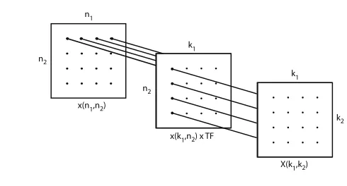
n

1

x(n

1,n2)

x(k₁,n₂) x TF

X(k₁,k₂) n2

n₂ k₁

k

1

[image:17.612.169.414.106.238.2]

k₂

Figure 3.1: Uncoupling of the Row and Column Calculations (Rectangles are Data Arrays)

The left 4-by-4 array is the mapped input data, the center array has the rows transformed, and the right array is the DFT array. The row DFTs and the column DFTs are independent of each other. The twiddle factors (TF) which are the centerW in (3.19), are the multiplications

which take place on the center array of Figure 3.1.

This uncoupling feature reduces the amount of arithmetic required and allows the results of each row DFT to be written back over the input data locations, since that input row will not be needed again. This is called in-place" calculation and it results in a large memory requirement savings.

An example of the type-two map used when the factors of N are relatively prime is given

for N = 15 as

n = 5n1+n2 (3.20)

k =k1+ 3k2 (3.21)

The residue reduction is again not explicitly needed. Although the factors 3 and 5 are relatively prime, use of the type-two map sets only one of the terms in (3.16) to zero. The DFT in (3.15) becomes

X =

4

X

n2=0 2

X

n1=0

x Wn1k1

3 W

n2k1

15 W

n2k2

5 (3.22)

which has the same form as (3.19), including the existence of the twiddle factors (TF). Here the inner sum is ve length-3 DFTs, one for each value of k1. This is illustrated in (3.2)

(18)

n₁

x(n₁,n₂)

x(k

1,n2)

X(k₁,k₂) n₂

n

2

k₁

[image:18.612.195.442.395.510.2]

k₁ k₂

Figure 3.2: Uncoupling of the Row and Column Calculations (Rectangles are Data Arrays)

An alternate illustration is shown in Figure 3.3 where the rectangles are the short length 3 and 5 DFTs.

Figure 3.3: Uncoupling of the Row and Column Calculations (Rectangles are Short DFTs)

The type-one map is illustrated next on the same length-15 example. This time the situation of (3.7) with the and" condition is used in (3.10) using an index map of

n= 5n1+ 3n2 (3.23)

and

(19)

The residue reduction is now necessary. Since the factors ofN are relatively prime and the

type-one map is being used, both terms in (3.16) are zero, and (3.15) becomes

^

X=

4

X

n2=0 2

X

n1=0 ^

x Wn1k1

3 W

n2k2

5 (3.25)

which is similar to (3.22), except that now the type-one map gives a pure two-dimensional DFT calculation with no TFs, and the sums can be done in either order. Figures Figure 3.2 and Figure 3.3 also describe this case but now there are no Twiddle Factor multiplications in the center and the resulting system is called a prime factor algorithm" (PFA).

The purpose of index mapping is to improve the arithmetic eciency. For example a direct calculation of a length-16 DFT requires 16^2 or 256 real multiplications (recall, one complex multiplication requires 4 real multiplications and 2 real additions) and an uncoupled version requires 144. A direct calculation of a length-15 DFT requires 225 multiplications but with a type-two map only 135 and with a type-one map, 120. Recall one complex multiplication requires four real multiplications and two real additions.

Algorithms of practical interest use short DFT's that require fewer thanN2 _{multiplications.}

For example, length-4 DFTs require no multiplications and, therefore, for the length-16 DFT, only the TFs must be calculated. That calculation uses 16 multiplications, many fewer than the 256 or 144 required for the direct or uncoupled calculation.

The concept of using an index map can also be applied to convolution to convert a lengthN =

N1N2 one-dimensional cyclic convolution into aN1 byN2 two-dimensional cyclic convolution

[46], [6]. There is no savings of arithmetic from the mapping alone as there is with the DFT, but savings can be obtained by using special short algorithms along each dimension. This is discussed in Algorithms for Data with Restrictions (Chapter 12) .

3.2 In-Place Calculation of the DFT and Scrambling

Because use of both the type-one and two index maps uncouples the calculations of the rows and columns of the data array, the results of each short lengthNi DFT can be written

back over the data as it will not be needed again after that particular row or column is transformed. This is easily seen from Figures Figure 3.1, Figure 3.2, and Figure 3.3 where the DFT of the rst row ofx(n1, n2)can be put back over the data rather written into a new

(20)

the output map (3.12). For example with a length-8 radix-2 FFT, the input index map is

n = 4n1+ 2n2+n3 (3.26)

which to satisfy (3.16) requires an output map of

k=k1+ 2k2+ 4k3 (3.27)

The in-place calculations will place the DFT results in the locations of the input map and these should be reordered or unscrambled into the locations given by the output map. Examination of these two maps shows the scrambled output to be in a bit reversed" order. For certain applications, this scrambled output order is not important, but for many applica-tions, the order must be unscrambled before the DFT can be considered complete. Because the radix of the radix-2 FFT is the same as the base of the binary number representation, the correct address for any term is found by reversing the binary bits of the address. The part of most FFT programs that does this reordering is called a bit-reversed counter. Examples of various unscramblers are found in [146], [60] and in the appendices.

The development here uses the input map and the resulting algorithm is called decimation-in-frequency". If the output rather than the input map is used to derive the FFT algorithm so the correct output order is obtained, the input order must be scrambled so that its values are in locations specied by the output map rather than the input map. This algorithm is called decimation-in-time". The scrambling is the same bit-reverse counting as before, but it precedes the FFT algorithm in this case. The same process of a post-unscrambler or pre-scrambler occurs for the in-place calculations with the type-one maps. Details can be found in [60], [56]. It is possible to do the unscrambling while calculating the FFT and to avoid a separate unscrambler. This is done for the Cooley-Tukey FFT in [192] and for the PFA in [60], [56], [319].

If a radix-2 FFT is used, the unscrambler is a bit-reversed counter. If a radix-4 FFT is used, the unscrambler is a base-4 reversed counter, and similarly for radix-8 and others. However, if for the radix-4 FFT, the short length-4 DFTs (butteries) have their outputs in bit-revered order, the output of the total radix-4 FFT will be in bit-reversed order, not base-4 reversed order. This means any radix-2n _{FFT can use the same radix-2 bit-reversed counter as an}

unscrambler if the proper butteries are used.

3.3 Eciencies Resulting from Index Mapping with the

DFT

(21)

The most general form of an uncoupled two-dimensional DFT is given by

X(k1, k2) =

N2−1 X

n2=0

{

N1−1 X

n1=0

x(n1, n2) f1(n1, n2, k1)} f2(n2, k1, k2) (3.28)

where the inner sum calculates N2 length-N1 DFT's and, if for a type-two map, the eects

of the TFs. If the number of arithmetic operations for a length-N DFT is denoted byF (N),

the number of operations for this inner sum isF =N2F(N1). The outer sum which givesN1

length-N2 DFT's requires N1F(N2) operations. The total number of arithmetic operations

is then

F =N2F (N1) +N1F(N2) (3.29)

The rst question to be considered is for a xed length N, what is the optimal relation of N1 and N2 in the sense of minimizing the required amount of arithmetic. To answer this

question, N1 and N2 are temporarily assumed to be real variables rather than integers. If

the short length-Ni DFT's in (3.28) and any TF multiplications are assumed to require Ni2

operations, i.e. F (Ni) = Ni2, "Eciencies Resulting from Index Mapping with the DFT"

(Section 3.3: Eciencies Resulting from Index Mapping with the DFT) becomes

F =N2N12 +N1N22 =N(N1+N2) =N N1+N N1−1

(3.30) To nd the minimum of F over N1, the derivative of F with respect to N1 is set to zero

(temporarily assuming the variables to be continuous) and the result requires N1 =N2.

dF/dN1 = 0 => N1 =N2 (3.31)

This result is also easily seen from the symmetry of N1 and N2 in N = N1N2. If a more

general model of the arithmetic complexity of the short DFT's is used, the same result is obtained, but a closer examination must be made to assure that N1 = N2 is a global

minimum.

If only the eects of the index mapping are to be considered, then the F (N) = N2 _{model is}

used and (3.31) states that the two factors should be equal. If there are M factors, a similar reasoning shows that all M factors should be equal. For the sequence of length

N =RM (3.32)

there are now M length-R DFT's and, since the factors are all equal, the index map must

be type two. This means there must be twiddle factors.

(22)

counts in (3.30) generalizes to

F =N

M

X

i=1

F (Ni)/Ni =N M F (R)/R (3.33)

for Ni =R

F =N lnR(N)F (R)/R= (N lnN) (F (R)/(RlnR)) (3.34)

This is a very important formula which was derived by Cooley and Tukey in their famous paper [89] on the FFT. It states that for a given R which is called the radix, the number of multiplications (and additions) is proportional to N lnN. It also shows the relation to the

value of the radix, R.

In order to get some idea of the best" radix, the number of multiplications to compute a length-R DFT is assumed to be F (R) = Rx_{. If this is used with (3.34), the optimal R can}

be found.

dF/dR= 0 => R =e1/(x−1) (3.35)

Forx= 2 this gives R=e, with the closest integer being three.

The result of this analysis states that if no other arithmetic saving methods other than index mapping are used, and if the length-R DFT's plus TFs require F =R2 _{multiplications, the}

optimal algorithm requires

F = 3N log₃N (3.36)

multiplications for a length N = 3M DFT. Compare this with N2 for a direct calculation

and the improvement is obvious.

While this is an interesting result from the analysis of the eects of index mapping alone, in practice, index mapping is almost always used in conjunction with special algorithms for the short length-Ni DFT's in (3.15). For example, if R = 2 or 4, there are no multiplications

required for the short DFT's. Only the TFs require multiplications. Winograd (see Winorad's Short DFT Algorithms (Chapter 7)) has derived some algorithms for short DFT's that require O(N) multiplications. This means that F(Ni) = KNi and the operation count F in "Eciencies Resulting from Index Mapping with the DFT" (Section 3.3: Eciencies

Resulting from Index Mapping with the DFT) is independent ofNi. Therefore, the derivative

of F is zero for all Ni. Obviously, these particular cases must be examined.

3.4 The FFT as a Recursive Evaluation of the DFT

(23)

terms of length-(N/4) DFTs. This allows the DFT to be calculated by a recursive algorithm with M recursions, giving the familiar order N log(N)arithmetic complexity.

Calculate the even indexed DFT values from (3.1) by:

C(2k) =

N−1

X

n=0

x(n) W_N2nk =

N−1

X

n=0

x(n) W_N/2nk (3.37)

C(2k) =

N/2−1

X

n=0

x(n) W_N2nk +

N−1

X

n=N/2

x(n) W_N/2nk (3.38)

C(2k) =

N/2−1

X

n=0

{x(n) + x(n+N/2)} W_N/2nk (3.39)

and a similar argument gives the odd indexed values as:

C(2k+ 1) =

N/2−1

X

n=0

{x(n) − x(n+N/2)} W_Nn W_N/2nk (3.40)

Together, these are recursive DFT formulas expressing the length-N DFT of x(n) in terms

of length-N/2 DFTs:

C(2k) =DFTN/2{x(n) + x(n+N/2)} (3.41) C(2k+ 1) =DFTN/2{[x(n) − x(n+N/2)]WNn} (3.42)

This is a decimation-in-frequency" (DIF) version since it gives samples of the frequency domain representation in terms of blocks of the time domain signal.

(24)

function c = dftr2(x)

% Recursive Decimation-in-Frequency FFT algorithm, csb 8/21/07 L = length(x);

if L > 1

L2 = L/2;

TF = exp(-j*2*pi/L).^[0:L2-1]; c1 = dftr2( x(1:L2) + x(L2+1:L)); c2 = dftr2((x(1:L2) - x(L2+1:L)).*TF); cc = [c1';c2'];

c = cc(:); else

c = x; end

Listing 3.1: DIF Recursive FFT for N = 2M

A DIT version can be derived in the form:

C(k) =DFTN/2{x(2n)} + WNkDFTN/2{x(2n+ 1)} (3.43) C(k+N/2) =DFTN/2{x(2n)} − WNkDFTN/2{x(2n+ 1)} (3.44)

(25)

function c = dftr(x)

% Recursive Decimation-in-Time FFT algorithm, csb L = length(x);

if L > 1

L2 = L/2;

ce = dftr(x(1:2:L-1)); co = dftr(x(2:2:L));

TF = exp(-j*2*pi/L).^[0:L2-1]; c1 = TF.*co;

c = [(ce+c1), (ce-c1)]; else

c = x; end

Listing 3.2: DIT Recursive FFT for N = 2M

Similar recursive expressions can be developed for other radices and and algorithms. Most recursive programs do not execute as eciently as looped or straight code, but some can be very ecient, e.g. parts of the FFTW.

Note a length-2M sequence will require M recursions, each of which will require N/2

(26)

(27)

Chapter 4

Polynomial Description of Signals

1

Polynomials are important in digital signal processing because calculating the DFT can be viewed as a polynomial evaluation problem and convolution can be viewed as polynomial multiplication [27], [261]. Indeed, this is the basis for the important results of Winograd discussed in Winograd's Short DFT Algorithms (Chapter 7). A length-N signal x(n) will

be represented by an N −1degree polynomial X(s)dened by

X(s) =

N−1

X

n=0

x(n) sn (4.1)

This polynomial X(s) is a single entity with the coecients being the values of x(n). It

is somewhat similar to the use of matrix or vector notation to eciently represent signals which allows use of new mathematical tools.

The convolution of two nite length sequences, x(n) and h(n), gives an output sequence

dened by

y(n) =

N−1

X

k=0

x(k) h(n−k) (4.2)

n = 0,1,2,· · · ,2N −1 where h(k) = 0 for k < 0. This is exactly the same operation as

calculating the coecients when multiplying two polynomials. Equation (4.2) is the same as

Y (s) =X(s) H(s) (4.3)

In fact, convolution of number sequences, multiplication of polynomials, and the multipli-cation of integers (except for the carry operation) are all the same operations. To obtain cyclic convolution, where the indices in (4.2) are all evaluated modulo N, the polynomial

multiplication in (4.3) is done modulo the polynomialP (s) =sN−1. This is seen by noting

that N = 0 mod N, therefore, sN _{= 1} _{and the polynomial modulus is}_sN ₋₁_.

(28)

4.1 Polynomial Reduction and the Chinese Remainder

Theorem

Residue reduction of one polynomial modulo another is dened similarly to residue reduction for integers. A polynomial F(s) has a residue polynomialR(s)modulo P (s) if, for a given F (s) and P(s), a Q(S) and R(s)exist such that

F(s) = Q(s)P(s) +R(s) (4.4)

with degree{R(s)}< degree{P (s)}. The notation that will be used is

R(s) = ((F(s)))_P_(s) (4.5)

For example,

(s+ 1) = s4+s3−s−1_(s2₋₁₎ (4.6) The concepts of factoring a polynomial and of primeness are an extension of these ideas for integers. For a given allowed set of coecients (values of x(n)), any polynomial has a

unique factored representation

F (s) =

M

Y

i=1 Fi(s)

ki (4.7)

where the Fi(s) are relatively prime. This is analogous to the fundamental theorem of

arithmetic.

There is a very useful operation that is an extension of the integer Chinese Remainder Theorem (CRT) which says that if the modulus polynomial can be factored into relatively prime factors

P (s) =P1(s) P2(s) (4.8)

then there exist two polynomials, K1(s) andK2(s), such that any polynomialF (s)can be

recovered from its residues by

F (s) =K1(s)F1(s) +K2(s)F2(s) modP (s) (4.9)

where F1 and F2 are the residues given by

F1(s) = ((F (s)))P1(s) (4.10) and

(29)

if the order of F(s) is less than P (s). This generalizes to any number of relatively prime

factors of P (s) and can be viewed as a means of representing F (s) by several lower degree

polynomials, Fi(s).

This decomposition of F (s) into lower degree polynomials is the process used to break a

DFT or convolution into several simple problems which are solved and then recombined using the CRT of (4.9). This is another form of the divide and conquer" or organize and share" approach similar to the index mappings in Multidimensional Index Mapping (Chapter 3). One useful property of the CRT is for convolution. If cyclic convolution ofx(n)and h(n)is

expressed in terms of polynomials by

Y (s) =H(s)X(s) mod P(s) (4.12)

where P (s) = sN ₋₁, and if _P ₍_s₎ is factored into two relatively prime factors _P ₌_P 1P2,

using residue reduction of H(s) and X(s) modulo P1 and P2, the lower degree residue

polynomials can be multiplied and the results recombined with the CRT. This is done by

Y (s) = ((K1H1X1+K2H2X2))P (4.13)

where

H1 = ((H))_P₁, X1 = ((X))_P₁, H2 = ((H))_P₂, X2 = ((X))_P₂ (4.14)

and K1 and K2 are the CRT coecient polynomials from (4.9). This allows two shorter

convolutions to replace one longer one.

Another property of residue reduction that is useful in DFT calculation is polynomial eval-uation. To evaluate F (s) ats=x, F(s)is reduced modulo s−x.

F (x) = ((F (s)))_s−x (4.15)

This is easily seen from the denition in (4.4)

F (s) =Q(s) (s−x) +R(s) (4.16)

Evaluatings =x gives R(s) =F (x)which is a constant. For the DFT this becomes

C(k) = ((X(s)))_s−Wk (4.17)

(30)

4.2 The DFT as a Polynomial Evaluation

The Z-transform of a number sequencex(n)is dened as

X(z) =

∞

X

n=0

x(n) z−n (4.18)

which is the same as the polynomial description in (4.1) but with a negative exponent. For a nite length-N sequence (4.18) becomes

X(z) =

N−1

X

n=0

x(n) z−n (4.19)

X(z) =x(0) +x(1)z−1+x(2)z−2+·+x(N −1)z−N+1 (4.20)

This N −1order polynomial takes on the values of the DFT of x(n)when evaluated at

z =ej2πk/N (4.21)

which gives

C(k) =X(z)|_z=ej2πk/N =

N−1

X

n=0

x(n) e−j2πnk/N (4.22)

In terms of the positive exponent polynomial from (4.1), the DFT is

C(k) = X(s)|_s=Wk (4.23)

where

W =e−j2π/N (4.24)

is an Nth root of unity (raising W to the Nth power gives one). The N values of the DFT

are found fromX(s)evaluated at the NNth _{roots of unity which are equally spaced around}

the unit circle in the complex s plane.

One method of evaluating X(z) is the so-called Horner's rule or nested evaluation. When

(31)

Another method for evaluatingX(s)is the residue reduction modulo s−Wk

as shown in (4.17). Each evaluation requiresN multiplications and therefore,N2 multiplications for the N values of C(k).

C(k) = ((X(s₎₎₎₍_s−Wk₎ (4.25)

A considerable reduction in required arithmetic can be achieved if some operations can be shared between the reductions for dierent values of k. This is done by carrying out the

residue reduction in stages that can be shared rather than done in one step for each k in

(4.25).

The N values of the DFT are values of X(s) evaluated at s equal to the N roots of the

polynomial P(s) =sN ₋₁ _{which are}_Wk_{. First, assuming} _N _{is even, factor} _P ₍_s₎ _as

P (s) = sN −1=P1(s) P2(s) = sN/2−1

sN/2+ 1 (4.26)

X(s) is reduced modulo these two factors to give two residue polynomials, X1(s) and X2(s). This process is repeated by factoring P1 and further reducing X1 then factoring P2

and reducingX2. This is continued until the factors are of rst degree which gives the desired

DFT values as in (4.25). This is illustrated for a length-8 DFT. The polynomial whose roots are Wk_{, factors as}

P (s) =s8−1 (4.27)

=

s4−1 s4+ 1

(4.28)

= s2−1 s2+ 1 s2−j s2+j (4.29)

= [(s−1) (s+ 1) (s−j) (s+j)] [(s−a) (s+a) (s−ja) (s+ja)] (4.30)

where a2 =j. Reducing X(s)by the rst factoring gives two third degree polynomials

X(s) =x0+x1s+x2s2+...+x7s7 (4.31)

gives the residue polynomials

X1(s) = ((X(s)))_(s4₋₁₎ = (x0+x4) + (x1+x5)s+ (x2+x6)s2+ (x3+x7)s3 (4.32) X2(s) = ((X(s)))(s4₊₁₎ = (x0−x4) + (x1−x5)s+ (x2−x6)s2+ (x3−x7)s3 (4.33)

(32)

(33)

Chapter 5

The DFT as Convolution or Filtering

1

A major application of the FFT is fast convolution or fast ltering where the DFT of the signal is multiplied term-by-term by the DFT of the impulse (helps to be doing nite impulse response (FIR) ltering) and the time-domain output is obtained by taking the inverse DFT of that product. What is less well-known is the DFT can be calculated by convolution. There are several dierent approaches to this, each with dierent application.

5.1 Rader's Conversion of the DFT into Convolution

In this section a method quite dierent from the index mapping or polynomial evaluation is developed. Rather than dealing with the DFT directly, it is converted into a cyclic convolution which must then be carried out by some ecient means. Those means will be covered later, but here the conversion will be explained. This method requires use of some number theory, which can be found in an accessible form in [234] or [262] and is easy enough to verify on one's own. A good general reference on number theory is [259].

The DFT and cyclic convolution are dened by

C(k) =

N−1

X

n=0

x(n) Wnk (5.1)

y(k) =

N−1

X

n=0

x(n) h(k−n) (5.2)

For both, the indices are evaluated moduloN. In order to convert the DFT in (5.1) into the

cyclic convolution of (5.2), the nk product must be changed to the k−n dierence. With

real numbers, this can be done with logarithms, but it is more complicated when working in a nite set of integers modulo N. From number theory [28], [234], [262], [259], it can be

shown that if the modulus is a prime number, a base (called a primitive root) exists such

(34)

that a form of integer logarithm can be dened. This is stated in the following way. IfN is

a prime number, a number r called a primitive roots exists such that the integer equation

n = ((rm))_N (5.3)

creates a unique, one-to-one map of theN−1member setm ={0, ..., N−2}and theN−1

member set n={1, ..., N −1}. This is because the multiplicative group of integers modulo

a prime, p, is isomorphic to the additive group of integers modulo (p−1) and is illustrated

for N = 5 below.

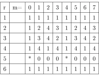
r m= 0 1 2 3 4 5 6 7

1 1 1 1 1 1 1 1 1

2 1 2 4 3 1 2 4 3

3 1 3 4 2 1 3 4 2

4 1 4 1 4 1 4 1 4

5 * 0 0 0 * 0 0 0

[image:34.612.208.404.245.395.2]

6 1 1 1 1 1 1 1 1

Table 5.1: Table of Integersn= ((rm)) modulo 5, [* not dened]

Table 5.1 is an array of values of rm _modulo _N _{and it is easy to see that there are two}

primitive roots, 2 and 3, and (5.3) denes a permutation of the integers n from the integers m (except for zero). (5.3) and a primitive root (usually chosen to be the smallest of those

that exist) can be used to convert the DFT in (5.1) to the convolution in (5.2). Since (5.3) cannot give a zero, a new length-(N-1) data sequence is dened from x(n) by removing the

term with index zero. Let

n=r−m (5.4)

and

k =rs (5.5)

where the term with the negative exponent (the inverse) is dened as the integer that satises

r−mrm_N = 1 (5.6)

IfN is a prime number, r−m always exists. For example, ((2−1))₅ = 3. (5.1) now becomes

C(rs) =

N−2

X

(35)

for s= 0,1, .., N−2, and

C(0) =

N−1

X

n=0

x(n) (5.8)

New functions are dened, which are simply a permutation in the order of the original functions, as

x'(m) =x r−m, C'(s) = C(rs), W'(n) = Wrn (5.9)

(5.7) then becomes

C'(s) =

N−2

X

m=0

x'(m) W'(s−m) + x(0) (5.10)

which is cyclic convolution of length N-1 (plusx(0)) and is denoted as

C'(k) = x'(k)∗W'(k) +x(0) (5.11)

Applying this change of variables (use of logarithms) to the DFT can best be illustrated from the matrix formulation of the DFT. (5.1) is written for a length-5 DFT as

          C(0) C(1) C(2) C(3) C(4)           =          

0 0 0 0 0 0 1 2 3 4 0 2 4 1 3 0 3 1 4 2 0 4 3 2 1

                    x(0) x(1) x(2) x(3) x(4)           (5.12)

where the square matrix should contain the terms ofWnk but for clarity, only the exponents nk are shown. Separating the x(0) term, applying the mapping of (5.9), and using the

primitive roots r= 2 (and r−1 = 3) gives

       C(1) C(2) C(4) C(3)        =       

1 3 4 2 2 1 3 4 4 2 1 3 3 4 2 1

              x(1) x(3) x(4) x(2)        +        x(0) x(0) x(0) x(0)        (5.13) and

C(0) =x(0) +x(1) +x(2) +x(3) +x(4) (5.14)

(36)

length-N DFT could be converted into a length-(N-1) cyclic convolution of a permutation of the data with a permutation of the W's. He also stated that a slightly more complicated version of the same idea would work for a DFT with a length equal to an odd prime to a power. The details of that theory can be found in [234], [169].

Until 1976, this conversion approach received little attention since it seemed to oer few advantages. It has specialized applications in calculating the DFT if the cyclic convolution is done by distributed arithmetic table look-up [77] or by use of number theoretic transforms [28], [234], [262]. It and the Goertzel algorithm [273], [62] are ecient when only a few DFT values need to be calculated. It may also have advantages when used with pipelined or vector hardware designed for fast inner products. One example is the TMS320 signal processing microprocessor which is pipelined for inner products. The general use of this scheme emerged when new fast cyclic convolution algorithms were developed by Winograd [405].

5.2 The Chirp Z-Transform (or Bluestein's Algorithm)

The DFT ofx(n)evaluates the Z-transform ofx(n)onN equally spaced points on the unit

circle in the z plane. Using a nonlinear change of variables, one can create a structure which

is equivalent to modulation and ltering x(n) by a chirp" signal. [34], [306], [298], [273],

[304], [62].

The mathematical identity (k−n)2 =k2₋₂_kn₊_n2 _gives

nk= n2−(k−n)2+k2/2 (5.15)

which substituted into the denition of the DFT in Multidimensional Index Mapping: Equa-tion 1 (3.1) gives

C(k) ={

N−1

X

n=0

h

x(n) Wn2/2i W−(k−n)2/2} Wk2/2 (5.16)

This equation can be interpreted as rst multiplying (modulating) the data x(n)by a chirp

sequence (Wn2_/2

, then convolving (ltering) it, then nally multiplying the lter output by the chirp sequence to give the DFT.

Dene the chirp sequence or signal as h(n) = Wn2/2 which is called a chirp because the

squared exponent gives a sinusoid with changing frequency. Using this denition, (5.16) becomes

C(n) = {[x(n) h(n)] ∗ h−1} h(n) (5.17)

(37)

This allows a prime length DFT to be calculated by a very ecient length-2M _{FFT. This}

becomes practical for large N when a particular non-composite (or N with few factors)

length is required.

As developed here, the chirp z-transform evaluates the z-transform at equally spaced points on the unit circle. A slight modication allows evaluation on a spiral and in segments [298], [273] and allows savings with only some input values are nonzero or when only some output values are needed. The story of the development of this transform is given in [304].

(38)

function y = chirpc(x); % function y = chirpc(x)

% computes an arbitrary-length DFT with the % chirp z-transform algorithm. csb. 6/12/91 %

N = length(x); n = 0:N-1; %Sequence length

W = exp(-j*pi*n.*n/N); %Chirp signal

xw = x.*W; %Modulate with chirp

WW = [conj(W(N:-1:2)),conj(W)]; %Construct filter

y = conv(WW,xw); %Convolve w filter

y = y(N:2*N-1).*W; %Demodulate w chirp

function y = chirp(x); % function y = chirp(x)

% computes an arbitrary-length Discrete Fourier Transform (DFT) % with the chirp z transform algorithm. The linear convolution % then required is done with FFTs.

% 1988: L. Arevalo; 11.06.91 K. Schwarz, LNT Erlangen; 6/12/91 csb. %

N = length(x); %Sequence length

L = 2^ceil(log((2*N-1))/log(2)); %FFT length

n = 0:N-1;

W = exp(-j*pi*n.*n/N); %Chirp signal

FW = fft([conj(W), zeros(1,L-2*N+1), conj(W(N:-1:2))],L);

y = ifft(FW.*fft(x.'.*W,L)); %Convolve using FFT

y = y(1:N).*W; %Demodulate

Figure 5.1

5.3 Goertzel's Algorithm (or A Better DFT Algorithm)

(39)

5.3.1 The First-Order Goertzel Algorithm

The polynomial whose values on the unit circle are the DFT is a slightly modied z-transform of x(n) given by

X(z) =

N−1

X

n=0

x(n)z−n (5.18)

which for clarity in this development uses a positive exponent . This is illustrated for a length-4 sequence as a third-order polynomial by

X(z) =x(3)z3+x(2)z2+x(1)z+x(0) (5.19)

The DFT is found by evaluating (5.18) at z =Wk, which can be written as

C(k) =X(z)|_z=Wk =DF T{x(n)} (5.20)

where

W =e−j2π/N (5.21)

The most ecient way of evaluating a general polynomial without any pre-processing is by Horner's rule" [208] which is a nested evaluation. This is illustrated for the polynomial in (5.19) by

X(z) ={[x(3)z+x(2)]z+x(1)}z+x(0) (5.22)

This nested sequence of operations can be written as a linear dierence equation in the form of

y(m) = z y(m−1) +x(N −m) (5.23)

with initial condition y(0) = 0, and the desired result being the solution at m =N. The

value of the polynomial is given by

X(z) = y(N). (5.24)

(5.23) can be viewed as a rst-order IIR lter with the input being the data sequence in reverse order and the value of the polynomial atzbeing the lter output sampled atm =N.

Applying this to the DFT gives the Goertzel algorithm [283], [269] which is

y(m) =Wky(m−1) +x(N −m) (5.25)

with y(0) = 0 and

(40)

where

C(k) =

N−1

X

n=0

x(n) Wnk. (5.27)

The owgraph of the algorithm can be found in [62], [269] and a simple FORTRAN program is given in the appendix.

When comparing this program with the direct calculation of (5.27), it is seen that the number of oating-point multiplications and additions are the same. In fact, the structures of the two algorithms look similar, but close examination shows that the way the sines and cosines enter the calculations is dierent. In (5.27), new sine and cosine values are calculated for each frequency and for each data value, while for the Goertzel algorithm in (5.25), they are calculated only for each frequency in the outer loop. Because of the recursive or feedback nature of the algorithm, the sine and cosine values are updated" each loop rather than recalculated. This results in 2N trigonometric evaluations rather than 2N2_{. It also results}

in an increase in accumulated quantization error.

It is possible to modify this algorithm to allow entering the data in forward order rather than reverse order. The dierence (5.23) becomes

y(m) =z−1y(m−1) +x(m−1) (5.28)

if (5.24) becomes

C(k) = zN−1y(N) (5.29)

for y(0) = 0. This is the algorithm programmed later.

5.3.2 The Second-Order Goertzel Algorithm

One of the reasons the rst-order Goertzel algorithm does not improve eciency is that the constant in the feedback or recursive path is complex and, therefore, requires four real multiplications and two real additions. A modication of the scheme to make it second-order removes the complex multiplications and reduces the number of required multiplications by two.

Dene the variableq(m) so that

y(m) =q(m)−z−1q(m−1). (5.30)

This substituted into the right-hand side of (5.23) gives

(41)

Combining (5.30) and (5.31) gives the second order dierence equation

q(m) = z+z−1

q(m−1)−q(m−2) +x(N −m) (5.32)

which together with the output (5.30), comprise the second-order Goertzel algorithm where

X(z) = y(N) (5.33)

for initial conditionsq(0) =q(−1) = 0.

A similar development starting with (5.28) gives a second-order algorithm with forward ordered input as

q(m) = z+z−1 q(m−1)−q(m−2) +x(m−1) (5.34)

y(m) =q(m)−z q(−1) (5.35)

with

X(z) = zN−1y(N) (5.36)

and for q(0) =q(−1) = 0.

Note that both dierence (5.32) and (5.34) are not changed if z is replaced with z−1, only

the output (5.30) and (5.35) are dierent. This means that the polynomial X(z) may be

evaluated at a particular z and its inverse z−1 from one solution of the dierence (5.32) or

(5.34) using the output equations

X(z) = q(N)−z−1q(N −1) (5.37)

and

X(1/z) = zN−1 (q(N)−z q(N −1)). (5.38)

Clearly, this allows the DFT of a sequence to be calculated with half the arithmetic since the outputs are calculated two at a time. The second-order DE actually produces a solution

q(m) that contains two rst-order components. The output equations are, in eect, zeros

(42)

5.3.3 Analysis of Arithmetic Complexity and Timings

Analysis of the various forms of the Goertzel algorithm from their programs gives the fol-lowing operation count for real multiplications and real additions assuming real data.

Algorithm Real Mults. Real Adds Trig Eval.

Direct DFT 4N2 ₄_N2 ₂_N2

First-Order 4N2 ₄_N2₋₂_N ₂_N

Second-Order 2N2+ 2N 4N2 2N

Second-Order 2 N2₊_N ₂_N2₊_N _N

Table 5.2

Timings of the algorithms on a PC in milliseconds are given in the following table.

Algorithm N = 125 N = 257

Direct DFT 4.90 19.83

First-Order 4.01 16.70

Second-Order 2.64 11.04

Second-Order 2 1.32 5.55

Table 5.3

These timings track the oating point operation counts fairly well.

5.3.4 Conclusions

Goertzel's algorithm in its rst-order form is not particularly interesting, but the two-at-a-time second-order form is signicantly faster than a direct DFT. It can also be used for any polynomial evaluation or for the DTFT at unequally spaced values or for evaluating a few DFT terms. A very interesting observation is that the inner-most loop of the Glassman-Ferguson FFT [124] is a rst-order Goertzel algorithm even though that FFT is developed in a very dierent framework.

In addition to oating-point arithmetic counts, the number of trigonometric function eval-uations that must be made or the size of a table to store precomputed values should be considered. Since the value of the Wnk terms in (5.23) are iteratively calculate in the IIR

(43)

It may be possible to further improve the eciency of the second-order Goertzel algorithm for calculating all of the DFT of a number sequence. Perhaps a fourth order DE could calculate four output values at a time and they could be separated by a numerator that would cancel three of the zeros. Perhaps the algorithm could be arranged in stages to give

anN log(N) operation count. The current algorithm does not take into account any of the

symmetries of the input index. Perhaps some of the ideas used in developing the QFT [53], [155], [158] could be used here.

5.4 The Quick Fourier Transform (QFT)

One stage of the QFT can use the symmetries of the sines and cosines to calculate a DFT more eciently than directly implementing the denition Multidimensional Index Mapping: Equation 1 (3.1). Similar to the Goertzel algorithm, the one-stage QFT is a betterN2 DFT

(44)

(45)

Chapter 6

Factoring the Signal Processing

Operators

1

A third approach to removing redundancy in an algorithm is to express the algorithm as an operator and then factor that operator into sparse factors. This approach is used by Tolimieri [382], [384], Egner [118], Selesnick, Elliott [121] and others. It is presented in a more general form in DFT and FFT: An Algebraic View (Chapter 8) The operators may be in the form of a matrix or a tensor operator.

6.1 The FFT from Factoring the DFT Operator

The denition of the DFT in Multidimensional Index Mapping: Equation 1 (3.1) can written as a matrix-vector operation by C =W X which, for N = 8 is

                  C(0) C(1) C(2) C(3) C(4) C(5) C(6) C(7)                   =                  

W0 W0 W0 W0 W0 W0 W0 W0

W0 _W1 _W2 _W3 _W4 _W5 _W6 _W7

W0 _W2 _W4 _W6 _W8 _W10 _W12 _W14

W0 W3 W6 W9 W12 W15 W18 W21

W0 _W4 _W8 _W12 _W16 _W20 _W24 _W28

W0 _W5 _W10 _W15 _W20 _W25 _W30 _W35

W0 W6 W12 W18 W24 W30 W36 W42

W0 _W7 _W14 _W21 _W28 _W35 _W42 _W49

                                    x(0) x(1) x(2) x(3) x(4) x(5) x(6) x(7)                   (6.1)

which clearly requires N2 = 64complex multiplications and N(N −1)additions. A

factor-ization of the DFT operator, W, givesW =F1 F2 F3 and C =F1 F2 F3 X or, expanded,

(46)







C

(0)

C

(4)

C

(2)

C

(6)

C

(1)

C

(5)

C

(3)

C

(7)







=







1

1 0

0 0

0

1

−

1 0

0 0

0

0 1

1 0

0 0

0

0 1

−

1 0

0 0

0

0 0

0 1

1 0

0

0 0

0 1

−

1 0

0

0 0

0 1

1

0

0 0

0 1

−

1













1

0

1

0

1

0

1

0

W

0

−

W

2

0

W

0

−

W

2

0

1

0

1

0

1

0

1

0

W

0

−

W

0

W

2

0

−

W

2







(6.2)                  

1 0 0 0 1 0 0 0 0 1 0 0 0 1 0 0 0 0 1 0 0 0 1 0 0 0 0 1 0 0 0 1

W0 ₀ ₀ ₀ ₋_W0 ₀ ₀ ₀

0 W1 ₀ ₀ ₀ ₋_W1 ₀ ₀

0 0 W2 0 0 0 −W2 0 0 0 0 W3 ₀ ₀ ₀ ₋_W3

                                    x(0) x(1) x(2) x(3) x(4) x(5) x(6) x(7)                   (6.3)

where theFi matrices are sparse. Note that each has 16 (or2N) non-zero terms andF2 and F3 have 8 (orN) non-unity terms. IfN = 2M, then the number of factors islog(N) = M. In

another form with the twiddle factors separated so as to count the complex multiplications we have                   C(0) C(4) C(2) C(6) C(1) C(5) C(3) C(7)                   =                  

1 1 0 0 0 0 0 0 1 −1 0 0 0 0 0 0 0 0 1 1 0 0 0 0 0 0 1 −1 0 0 0 0 0 0 0 0 1 1 0 0 0 0 0 0 1 −1 0 0 0 0 0 0 0 0 1 1 0 0 0 0 0 0 1 −1

(47)

                 

1 0 0 0 0 0 0 0 0 1 0 0 0 0 0 0 0 0 W0 0 0 0 0 0 0 0 0 W2 0 0 0 0 0 0 0 0 1 0 0 0 0 0 0 0 0 1 0 0 0 0 0 0 0 0 W0 ₀

0 0 0 0 0 0 0 W2

                                   

1 0 1 0 0 0 0 0 0 1 0 1 0 0 0 0 1 0 −1 0 0 0 0 0 0 1 0 −1 0 0 0 0 0 0 0 0 1 0 1 0 0 0 0 0 0 1 0 1 0 0 0 0 1 0 −1 0 0 0 0 0 0 1 0 −1

                  (6.5)                  

1 0 0 0 0 0 0 0 0 1 0 0 0 0 0 0 0 0 1 0 0 0 0 0 0 0 0 1 0 0 0 0 0 0 0 0 W0 ₀ ₀ ₀

0 0 0 0 0 W1 0 0 0 0 0 0 0 0 W2 ₀

0 0 0 0 0 0 0 W3

                                   

1 0 0 0 1 0 0 0 0 1 0 0 0 1 0 0 0 0 1 0 0 0 1 0 0 0 0 1 0 0 0 1 1 0 0 0 −1 0 0 0 0 1 0 0 0 −1 0 0 0 0 1 0 0 0 −1 0 0 0 0 1 0 0 0 −1

                                    x(0) x(1) x(2) x(3) x(4) x(5) x(6) x(7)                   (6.6)

which is in the form C = A1 M1 A2 M2 A3 X described by the index map. A1, A2, and A3 each represents 8 additions, or, in general,N additions. M1 and M2 each represent 4 (or N/2) multiplications.

This is a very interesting result showing that implementing the DFT using the factored form requires considerably less arithmetic than the single factor denition. Indeed, the form of the formula that Cooley and Tukey derived showing that the amount of arithmetic required by the FFT is on the order ofN log(N)can be seen from the factored operator formulation.

Much of the theory of the FFT can be developed using operator factoring and it has some advantages for implementation of parallel and vector computer architectures. The eigenspace approach is somewhat of the same type [18].

6.2 Algebraic Theory of Signal Processing Algorithms

(48)

(49)

Chapter 7

Winograd's Short DFT Algorithms

1

In 1976, S. Winograd [406] presented a new DFT algorithm which had signicantly fewer multiplications than the Cooley-Tukey FFT which had been published eleven years earlier. This new Winograd Fourier Transform Algorithm (WFTA) is based on the type- one index map from Multidimensional Index Mapping (Chapter 3) with each of the relatively prime length short DFT's calculated by very ecient special algorithms. It is these short algo-rithms that this section will develop. They use the index permutation of Rader described in the another module to convert the prime length short DFT's into cyclic convolutions. Winograd developed a method for calculating digital convolution with the minimum number of multiplications. These optimal algorithms are based on the polynomial residue reduction techniques of Polynomial Description of Signals: Equation 1 (4.1) to break the convolution into multiple small ones [29], [235], [263], [416], [408], [197].

The operation of discrete convolution dened by

y(n) = X

k

h(n−k) x(k) (7.1)

is called a bilinear operation because, for a xed h(n), y(n) is a linear function of x(n)

and for a xed x(n) it is a linear function of h(n). The operation of cyclic convolution is

the same but with all indices evaluated modulo N.

Recall from Polynomial Description of Signals: Equation 3 (4.3) that length-N cyclic convo-lution of x(n) and h(n) can be represented by polynomial multiplication

Y (s) =X(s) H(s) mod sN −1 (7.2)

This bilinear operation of (7.1) and (7.2) can also be expressed in terms of linear matrix operators and a simpler bilinear operator denoted byo which may be only a simple

element-by-element multiplication of the two vectors [235], [197], [212]. This matrix formulation

(50)

is

Y =C[AXoBH] (7.3)

whereX,H and Y are length-N vectors with elements ofx(n),h(n)andy(n)respectively.

The matrices A and B have dimension M x N , and C is N x M with M ≥ N. The

elements of A, B, and C are constrained to be simple; typically small integers or rational

numbers. It will be these matrix operators that do the equivalent of the residue reduction on the polynomials in (7.2).

In order to derive a useful algorithm of the form (7.3) to calculate (7.1), consider the polyno-mial formulation (7.2) again. To use the residue reduction scheme, the modulus is factored into relatively prime factors. Fortunately the factoring of this particular polynomial,sN−1,

has been extensively studied and it has considerable structure. When factored over the rationals, which means that the only coecients allowed are rational numbers, the factors are called cyclotomic polynomials [29], [235], [263]. The most interesting property for our purposes is that most of the coecients of cyclotomic polynomials are zero and the others are plus or minus unity for degrees up to over one hundred. This means the residue reduction will generally require no multiplications.

The operations of reducing X(s) and H(s) in (7.2) are carried out by the matrices A and B in (7.3). The convolution of the residue polynomials is carried out by the o operator and

the recombination by the CRT is done by the C matrix. More details are in [29], [235],

[263], [197], [212] but the important fact is the A and B matrices usually contain only zero

and plus or minus unity entries and the C matrix only contains rational numbers. The only

general multiplications are those represented by o. Indeed, in the theoretical results from

computational complexity theory, these real or complex multiplications are usually the only ones counted. In practical algorithms, the rational multiplications represented by C could

be a limiting factor.

The h(n) terms are xed for a digital lter, or they represent the W terms from

Multidi-mensional Index Mapping: Equation 1 (3.1) if the convolution is being used to calculate a DFT. Because of this, d = BH in (7.3) can be precalculated and only the A and C

opera-tors represent the mathematics done at execution of the algorithm. In order to exploit this feature, it was shown [416], [197] that the properties of (7.3) allow the exchange of the more complicated operator C with the simpler operatorB. Specically this is given by

Y =C[AXoBH] (7.4)

Y' =BT

AXoCTH'

(7.5) whereH' has the same elements asH, but in a permuted order, and likewiseY' andY. This

very important property allows precomputing the more complicated CT_H' in (7.5) rather

(51)

BecauseBHorCT_H_{' can be precomputed, the bilinear form of (7.3) and (7.5) can be written}

as a linear form. If an M x M diagonal matrix D is formed from d =CTH, or in the case

of (7.3), d=BH, assuming a commutative property for o, (7.5) becomes

Y'=BTDAX (7.6)

and (7.3) becomes

Y =CDAX (7.7)

In most cases there is no reason not to use the same reduction operations on X and H,

therefore, B can be the same asA and (7.6) then becomes

Y' =ATDAX (7.8)

In order to illustrate how the residue reduction is carried out and how the A matrix is obtained, the length-5 DFT algorithm started in The DFT as Convolution or Filtering: Matrix 1 (5.12) will be continued. The DFT is rst converted to a length-4 cyclic convolution by the index permutation from The DFT as Convolution or Filtering: Equation 3 (5.3) to give the cyclic convolution in The DFT as Convolution or Filtering (Chapter 5). To avoid confusion from the permuted order of the datax(n)in The DFT as Convolution or Filtering

(Chapter 5), the cyclic convolution will rst be developed without the permutation, using the polynomial U(s)

U(s) = x(1) +x(3)s+x(4)s2+x(2)s3 (7.9) U(s) = u(0) +u(1)s+u(2)s2+u(3)s3 (7.10)

and then the results will be converted back to the permuted x(n). The length-4 cyclic

convolution in terms of polynomials is

Y (s) =U(s) H(s) mod s4−1 (7.11)

and the modulus factors into three cyclotomic polynomials

s4−1 = s2−1 s2+ 1 (7.12)

= (s−1) (s+ 1) s2+ 1 (7.13)

=P1 P2 P3 (7.14)

Both U(s) and H(s) are reduced modulo these three polynomials. The reduction modulo

P1 and P2 is done in two stages. First it is done modulo(s2−1), then that residue is further

reduced modulo (s−1) and (s+ 1).

(52)

U'(s) = ((U(s)))_(s2₋₁₎ = (u0+u2) + (u1+u3)s (7.16)

U1 (s) = U'(s)_P

1 = (u0+u1+u2+u3) (7.17)

U2 (s) = U'(s)_P

2 = (u0−u1+u2−u3) (7.18)

U3 (s) = ((U(s)))_P

3 = (u0−u2) + (u1−u3)s (7.19) The reduction in (7.16) of the data polynomial (7.15) can be denoted by a matrix operation on a vector which has the data as entries.





1 0 1 0 0 1 0 1

         u0 u1 u2 u3        =  

u0+u2

u1+u3



 (7.20)

and the reduction in (7.19) is





1 0 −1 0 0 1 0 −1