SQCD: A Geometric Apercu

      

City, University of London Institutional Repository

Citation:

Gray, J., Hanany, A., He, Y., Jejjala, V. and Mekareeya, N. (2008). SQCD: A Geometric Apercu. Journal of High Energy Physics, 2008(JHEP05), 099 - 099. doi: 10.1088/1126-6708/2008/05/099

This is the unspecified version of the paper.

This version of the publication may differ from the final published

version.

Permanent repository link:

http://openaccess.city.ac.uk/878/

Link to published version:

http://dx.doi.org/10.1088/1126-6708/2008/05/099

Copyright and reuse: City Research Online aims to make research

outputs of City, University of London available to a wider audience.

Copyright and Moral Rights remain with the author(s) and/or copyright

holders. URLs from City Research Online may be freely distributed and

linked to.

City Research Online: http://openaccess.city.ac.uk/ [email protected]

arXiv:0803.4257v2 [hep-th] 29 Aug 2008

Preprint typeset in JHEP style - PAPER VERSION

SQCD: A Geometric Aper¸

cu

James Graya and Yang-Hui Heabc

a

Rudolf Peierls Centre for Theoretical Physics, Oxford University, 1 Keble Road, OX1 3NP, U.K.

b

Collegium Mertonense in Academia Oxoniensis, Oxford, OX1 4JD, U.K.

c

Mathematical Institute, Oxford University, 24-29 St. Giles’, Oxford, OX1 3LB, U.K.

E-mail: [email protected], [email protected]

Amihay Hanany and Noppadol Mekareeya Theoretical Physics Group, The Blackett Laboratory Imperial College London, Prince Consort Road London, SW7 2AZ, U.K.

E-mail: [email protected], [email protected]

Vishnu Jejjala

Institut des Hautes ´Etudes Scientifiques,

35, Route de Chartres, 91440 Bures-sur-Yvette, France

E-mail: [email protected]

Abstract: _{We take new algebraic and geometric perspectives on the old subject of}

Contents

1. Introduction and Summary 1

2. The Moduli Space of N = 1 Gauge Theories 4

2.1 Moduli Spaces Using Computational Algebraic Geometry 5 2.2 Primary Decomposition and Hilbert Series 5

3. Supersymmetric QCD 7

3.1 The Case of Nf < Nc 8

3.2 The Case of Nf ≥Nc 10

3.2.1 The Case of Nf =Nc 11

3.3 Special Case: Nc = 2 12

3.4 The Algebraic Geometry of SQCD Vacuum 14 3.4.1 The Example of (Nf = 4, Nc = 2) 14

3.4.2 Other Examples 15

3.4.3 U(1)-Charges and Weighted Embeddings 16 3.4.4 Further Geometric Properties 17 3.4.5 The SQCD Vacuum Is Calabi–Yau 18 3.4.6 The Quantum Moduli Space of SQCD 19 3.4.7 The Nf < Nc theories 19

3.4.8 The Nf ≥Nc theories 20

4. Counting Gauge Invariants: the Plethystic Programme and Molien–

Weyl formula 20

4.1 The Case of Two Colours: Nc = 2 23

4.1.1 The Example of (Nf = 1, Nc = 2) 23

4.1.2 (Nf, Nc = 2) with Arbitrary Flavours 24

4.1.3 Plethystic Logarithms andM(Nf,Nc=2) 26

4.2 The Case of Three Colours: Nc = 3 26

4.2.1 (Nf, Nc = 3) with Arbitrary Flavours 27

4.2.2 Plethystic Logarithms andM(Nf,Nc=3) 28

5. Character Expansion and Global Symmetries 30

5.1 The Case of Two Colours Revisited 31 5.1.1 The Example of (Nf = 2, Nc = 2) 31

5.1.2 The Example of (Nf >1, Nc = 2) 33

5.1.3 From SU(2Nf) to SU(Nf)L×SU(Nf)R 34

5.2 Character Expansion for General (Nf, Nc) 36

5.2.1 The Example of (Nf = 2, Nc = 3) 38

5.2.2 The Example of (Nf = 3, Nc = 3) 39

5.2.3 The Example of (Nf = 4, Nc = 3) 40

1. Introduction and Summary

Supersymmetric Quantum Chromodynamics (SQCD) is one of the most extensively studied subjects in modern theoretical physics. Investigations within this laboratory have provided a point of contact between field theory, phenomenology, string theory, and mathematics. The moduli space of SQCD typically consists of continuous vacuum solutions of the field equations. The lifting of the classical vacuum by quantum correc-tions [1], the phase structure [2, 3], dualities [4], etc., have all afforded powerful insights into the theory. The excellent reviews and lectures [5, 6, 7, 8] collect this work and provide references to the original literature. Here, we take a novel perspective on this well established subject.

Observing that the vacuum moduli space of a supersymmetric gauge theory, due to its subtle structure, is best described by the language of algebraic varieties, we employ techniques from algebraic geometry to gain physical insight. This is very much in light of the recent percolation of computational and algorithmic algebraic geometry into the study of field theory [9, 10, 11, 12] as well as the emergence of the plethystic programme for systematically studying chiral gauge invariant operators using geometric methods [13, 14, 15, 16, 17, 18, 19, 20, 21, 22, 23]. This new, geometric aper¸cu, as we demonstrate in this paper, is a remarkably fruitful development. Geometric quantities such as Hilbert series, perhaps unfamiliar to the physics community, provide a new understanding of the theory and allow us to easily perform calculations that are cumbersome using standard methods.

Our focus in this paper isN = 1 SQCD withSU(Nc) gauge group andNf flavours

transformation properties under the SU(Nf)L × SU(Nf)R × U(1)B ×U(1)R global

symmetry. In these initial investigations, we shall concentrate our attention on the case with a vanishing superpotential. The vacuum space is conveniently described by polynomial equations written in terms of variables which are the holomorphic gauge invariant operators (GIOs) of the theory, that is to say, the mesons, baryons, and antibaryons.

ForNf < Nc, the gauge group is spontaneously broken in the vacuum to SU(Nc−

Nf). The only GIOs are mesonic, and these parametrise a classical moduli space

that is N2

f-dimensional. However, at the quantum mechanical level, non-perturbative

corrections lift the space of classical vacuum solutions completely via the dynamically generated ADS superpotential, and consequently there is no quantum moduli space for Nf < Nc.

For Nf ≥ Nc, the gauge symmetry is completely broken at a generic point in the

classical moduli space, which is (2NcNf −Nc2 + 1)-dimensional. The moduli space

is described by relations (syzygies) amongst mesonic operators and baryonic opera-tors. With the incorporation of quantum corrections, the classical moduli space for the Nf = Nc theories which contained the singularity at the origin is deformed to a

smooth hypersurface, whereas the quantum moduli space for the Nf > Nc theories is

identical with the classical one. Although the precise classical relations get modified by quantum corrections for Nf = Nc, quantum corrections do not affect the number

of chiral operators at each order of quarks and antiquarks. Therefore, the generating functions which count the gauge invariant operators in the Nf ≥ Nc theories are not

changed by quantum corrections.

Algorithmic algebraic geometry, the plethystic programme, the Molien–Weyl for-mula, and character expansions yield a more refined understanding of textbook facts about the structure of the SQCD vacuum. In addition, the geometric invariants of the moduli space of vacua capture a vast quantity of non-trivial information about the phenomenology of the gauge theory. Algebraic geometry therefore supplies a powerful new window into the structure of SQCD.

To facilitate the reading of this paper, we have highlighted the key points in bold font as Observations. Below, we collect the main results of our geometric aper¸cu of SQCD.

Outline and Key Points:

primary decomposition, which breaks the moduli space up into irreducible pieces, and the Hilbert series, which enumerates the chiral GIOs of the theory.

• In Section 3, we examine M(Nf,Nc), the classical moduli space of vacua of SQCD,

for various values ofNc andNf. We characterise the vacuum varieties in terms of

their defining equations and find them to be affine cones over (compact) weighted projective varieties. For Nf < Nc, M(Nf,Nc) ≃ CN

2

f (Observations 3.1 and 3.2).

For Nf =Nc, the moduli space is a complete intersection (in fact a single

hyper-surface) in CNf2+2 with a rational function as its Hilbert series (Observations 3.5

and 3.6). For Nf > Nc, the moduli space is a non-complete intersection of

poly-nomial relations (syzygies) amongst the GIOs. We also analyse the case of two colours in detail. Using characters of its global symmetry the generating function is written for arbitrary number of flavours (Observation 3.8 and Equation (3.18)).

• We find the precise weighted projective variety over which M(Nf,Nc) is an affine

cone and tabulate the first few Hilbert series for these spaces in Table 3. Moreover, we find in all case studies that M(Nf,Nc) is irreducible using primary

decomposi-tion and conjecture this to hold in general (Observadecomposi-tion 3.11).

• Importantly, we establish that M(Nf,Nc) is Calabi–Yau (Observation 3.13).

This follows from the fact that the Hilbert series has palindromic numerator. We outline a proof based on an independent argument.

• We discuss the quantum moduli space of SQCD in Section 3.4.6. For Nf <

Nc, there is no supersymmetric vacuum. The classical vacuum geometry is an

auxiliary space useful for counting gauge invariant operators. For Nf ≥Nc, the

Hilbert series computed in the classical theory is quantum mechanically exact.

• In Section 4, we obtain an analytic formula for the generating function of GIOs in SQCD with fully refined chemical potentials corresponding to quarks and an-tiquarks; this is a refined version of the Hilbert series of M(Nf,Nc). The formula

is in the form of the Molien–Weyl integral, as given in Equation (4.9). The results are in complete agreement with those obtained in Section 3 using algo-rithmic algebraic geometry and also affirm the fact that the generating function (Hilbert series) encodes the defining relations of the moduli space of vacua. Thus, the results of Section 4 verify that the geometry of the classical moduli space of

N = 1 SQCD encapsulates the structure of the chiral ring of BPS gauge invariant operators. Ours is the first systematic analysis undertaken for (Nc ≥2, Nf >3).1

1_{Earlier works [24, 25] contain some of the results for N}

• In Section 5, we synthesise our prior results using representation theory and the character expansion.

It proves useful to write the Hilbert series in terms of characters. This permits the generalisation of our results to an arbitrary number of colours and flavours. Subsequently, we obtain an important result, namely the full character expansion of the generating function for any values of Nf and Nc (Equations (5.1), (5.2)

and (5.3)). We can interpret the coefficients as Young Tableaux and arrive at selection rules (Observation 5.6) for the terms appearing in the expansion.

2. The Moduli Space of

N

= 1

Gauge Theories

We begin by reviewing how to algorithmically compute the classical supersymmetric vacuum space of anN = 1 gauge theory. Consider a general N = 1 theory of the form

S =

Z

d4x

Z

d4θ Φ†_ieVΦi+

1 16g2

Z

d2θ trWαWα+

Z

d2θ W(Φi) + h.c.

.

(2.1) The Φiare chiral superfields in a representationRiof the gauge groupG;V is the vector

superfield in the Lie algebra g; Wα = −1₄D 2

e−V_D

αeV is the gauge field strength; and

W(Φi) is the superpotential, which is holomorphic in Φi. Integrating over superspace,

the scalar potential becomes

V(φi, φi) =

X

i

∂W ∂φi

2

+1 2

X

a

g2 X

i

φ†_iTaφi

!2

, (2.2)

where φi is the lowest component of Φi, Ta are the generators of G, and g is the

gauge coupling.2 _{The potential is minimised on loci where it vanishes. The condition}

V(φi, φi) = 0 yields the supersymmetry preserving D-term and F-term constraints:

Da=X

i

φ†_iTaφi = 0 (D-terms) ;

fi =

∂W ∂φi

= 0 (F-terms). (2.3)

There is a D-term for each generatorTa_{of the gauge group and an F-term for each field.}

Thevacuum moduli space Mis the space of solutions to D- and F-flatness constraints. The action (2.1) has an enormous gauge redundancy that we can most easily elim-inate by working with GC_{, the complexification of the gauge group.}3 _{The F-flatness}

2_{We neglect Fayet–Iliopoulos terms associated toU(1) factors inGin this discussion but these can}

be easily incorporated.

conditions are holomorphic and invariant underGC_{. The D-flatness conditions are}

triv-ial gauge fixing parameters. It is a standard fact inN = 1 gauge theory that for any solution of the F-term equations, there exists a unique solution to the D-term equations in the completion of the orbit of the complexified gauge group. The moduli space is, therefore, the symplectic quotient

M=F//GC , (2.4)

where F is the space of F-flat field configurations. The set of holomorphic gauge invariant operators of the theory forms a basis for the D-orbits. The geometry of the vacuum is therefore an algebraic variety specified by polynomial equations in the GIOs.

2.1 Moduli Spaces Using Computational Algebraic Geometry

Recasting the computation of the vacuum geometry into efficient, algorithmic tech-niques in algebraic geometry is the subject of [9, 10, 11]. For completeness, we briefly recollect the method.

1. The F-flatness conditions are an ideal of the polynomial ring C_{[φ1, . . . , φn]:}

hfi=1,...,ni=h

∂W ∂φi

i . (2.5)

2. From the matter fields{Φ1, . . . ,Φn}, we construct a basis of GIOsρ={ρ1, . . . , ρk}.

The ρj are, by construction, uncharged under GC. The definitions of the GIOs

in terms of the fields defines a natural ring map:

C_{[φ1, . . . , φn]−→}ρ C_{[ρ1, . . . , ρk] . (2.6)}

3. The moduli space M is then the image of the ring map:

C_{[φ1, . . . , φn]} {F =hf1, . . . , fni}

ρ

−→C_{[ρ1, . . . , ρk] . (2.7)}

That is to say, M ≃ Im(ρ) is an ideal of C_{[ρ1, . . . , ρk] which corresponds to an}

affine variety inCk_{. Practically, the image of the map (2.7), and thus the vacuum}

geometry M, can be calculated using Gr¨obner basis methods as implemented in the algebraic geometry software packages Macaulay 2 [26] and Singular [27].

2.2 Primary Decomposition and Hilbert Series

Extracting Irreducible Pieces: The moduli space may not be a single irreducible piece, but rather, may be composed of various components. This is a well recognised feature in supersymmetric gauge theories. The different components are typically called

branches of the moduli space, such as Coulomb or Higgs branches. It is an

impor-tant task to identify the different components since the massless spectrum on each component has its own unique features.

We are thus naturally led to look for a process to extract the various irreducible components of the vacuum space. Such an algorithm exists and, in the mathematics literature, is calledprimary decompositionof the ideal corresponding to the moduli space. Algorithms for performing primary decomposition have been extensively studied in computational algebraic geometry (cf., for example, [28] and for implementations, [26, 27]). A convenient package which calls the computational algebraic geometry programme Singular externally but which is based upon the Mathematica interface,

which perhaps is more familiar to physicists, is STRINGVACUA [11]. In fact, using [11], the primary decomposition of string vacua of phenomenological significance, is one of the subjects of [12].

The Hilbert Series: As being pointed out in [13, 17, 19, 23], the Hilbert series is a key to the problem of counting GIOs in a gauge theory. Mathematically, it is also an important quantity that characterises an algebraic variety. Although it is not a topo-logical invariant as it depends on the embedding under consideration, it nevertheless encodes many important properties of the variety once the embedding is known. We recall that for a varietyMin C_{[x1, ..., xk], the Hilbert series is the generating function}

for the dimension of the graded pieces:

H(t;M) =

∞

X

i=−∞

(dimCMi)ti , (2.8)

whereMi, thei-th graded piece ofMcan be thought of as the number of independent

degree i (Laurent) polynomials on the variety M. It will be understood henceforth that we are speaking about complex dimension, and we shall simplify our notation accordingly.

A useful property of H(t) is that it is a rational function in t and can be written in two ways:

H(t;M) =

( _Q(t)

(1−t)k , Hilbert series of the first kind ; P(t)

(1−t)dim(M) , Hilbert series of the second kind .

(2.9)

One of the important expansions of the Hilbert series is a Laurent expansion about 1, and the coefficient of the leading pole can be interpreted as the volume of the dual Sasaki–Einstein manifold in the AdS/CFT context which in the case of the Calabi–Yau three-fold, this volume is related to the central charges of supersymmetric gauge theory (cf. [29, 23]). Although it is not clear for general SQCD what the volume means, we can nevertheless perform such an expansion. For a Hilbert series in second form,

H(t;M) = P(1)

(1−t)dim(M) +. . . , P(1) = degree(M) . (2.10)

In particular,P(1) always equals the degree of the variety.4

3. Supersymmetric QCD

Having set the stage with the necessary geometric background, let us specialise to the gauge theory in which we are chiefly interested. In this section, let us fix notation by introducing the content of the theory. Let there also be no superpotential, W = 0. Thus there will be no F-terms, and the vacuum space is determined exclusively by the D-terms and is realised as the relations among the GIOs of the theory.

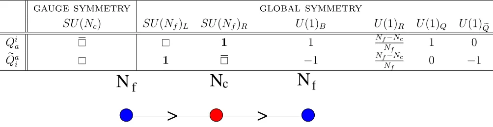
We specify SQCD with gauge group SU(Nc) and Nf flavours by the ordered pair

(Nf, Nc). This theory has quarks Qia and antiquarks Qeai, with flavour indices i =

1, . . . , Nf and colour indicesa = 1, . . . , Nc. Thus, there is a total of 2NcNf chiral degrees

of freedom from the quarks and antiquarks. Their quantum numbers are summarised in Table 1 where denotes the fundamental representation and 1 denotes the trivial representation of the group.

Notation for irreducible representations of SU(n): We can represent an

irre-ducible representation of SU(n) by a Young diagram. Let λi be the length of the

i-th row (1 ≤ i ≤ n − 1) and let ai = λi − λi+1 be the differences of lengths of

rows. Henceforth, we denote such a representation by the notation [a1, a2, . . . , an−1].

For example, [1,0, . . . ,0] represents the fundamental representation, [0, . . . ,0,1] repre-sents the antifundamental representation, and [1,0, . . . ,0,1] (where the second 1 is in the (n−1)-th position) represents the adjoint representation. For the product group SU(n)×SU(n), we use the notation [. . .;. . .] where the (n−1)-tuple to the left of the ‘;’ is the representation of the left SU(n), and likewise on the right.

4_{We recall that when an ideal is described by a single polynomial, the degree of the variety is simply}

gauge symmetry global symmetry

SU(Nc) SU(Nf)L SU(Nf)R U(1)B U(1)R U(1)Q U(1)Qe

Qi

a 1 1

Nf−Nc

Nf 1 0

e

Qa

i 1 −1

Nf−Nc

[image:11.612.86.588.80.210.2]

Nf 0 −1

Table 1: _{The gauge and global symmetries of SQCD and the quantum numbers of the chiral}

supermultiplets. The quarks areQi_awhile the antiquarks areQea_i. We also draw it as a quiver theory. The central (red) node represents theSU(Nc) gauge symmetry while the two (blue) end nodes

denote the globalU(N_f) symmetries. Each node gives rise to a baryonicU(1) global symmetry, one of which is redundant. We thus haveU(1)_Q,Q˜ that combine into the non-anomalous U(1)B

(sum) and anomalousU(1)A (difference).

3.1 The Case of Nf < Nc

In this situation, at a generic point in the moduli space, the SU(Nc) gauge symmetry

is partially broken toSU(Nc −Nf). Thus, there are

(N_c2−1)−((Nc−Nf)2−1) = 2NcNf −Nf2 (3.1)

broken generators. The total number of degrees of freedom of the system is, of course, unaffected by this spontaneous symmetry breaking and the massive gauge bosons each eat one degree of freedom from the chiral matter via the Higgs effect. Therefore, of the original 2NcNf chiral supermultiplets, only Nf2 singlets are left massless. Hence, the

dimension of the moduli space of vacua is

dim MNf<Nc

=N2

f . (3.2)

We can describe the remaining N2

f light degrees of freedom in a gauge invariant way

by anNf ×Nf matrix field, composed of the mesons:

Mi

j =QiaQeaj (mesons) . (3.3)

The Mi

j are clearly gauge invariant as the colour index on the right hand side is

summed. There are no baryons since Nf < Nc. Thus, (3.3) constitute the only GIOs.

the bifundamental representation [1,0, . . .; 0, . . . ,1] of the SU(Nf)L×SU(Nf)R global

symmetry. We note that for the Nf < Nc theory, there are no relations (constraints)

between mesons. Phrasing this geometrically, and noting the dimension from (3.2), we have that

Observation 3.1. The moduli space is freely generated: there are no relations among the generators. The space MNf<Nc is, in fact, nothing but CN

2 f.

GIOs composed of k quarks and k antiquarks must be of the form: Mi1 j1 . . . M

ik jk.

Because of the symmetry under the interchange of any two M’s, this product trans-forms in the representation Symk[1,0, . . . ,0; 0, . . . ,1] of theSU(Nf)L×SU(Nf)Rglobal

symmetry. A computation of this k-th symmetric product for a bifundamental repre-sentation is rather amusing and gives

Symk[1,0, . . . ,0; 0, . . . ,1] =

Nf X i=1 ∞ X ni=0

n1, n2, . . . , nNf−1;nNf−1, . . . , n2, n1

δ

 k−

Nf X j=1 jnj   , (3.4) where5 _{the only dependence on k comes from the constraint on the number of boxes}

in the Young diagram which is represented by the δ function. The total dimension of these representations gives

1 k!(N

2

f)(Nf2 + 1). . .(Nf2+k−1) =

N2

f +k−1

k

(3.5)

independent components. We can sum this to give a generating function for the gauge invariants and obtain:

Observation 3.2. The generating function of GIOs for SQCD with Nf < Nc is

gNf<Nc(t) =

∞

X

k=0

N2

f +k−1

k

t2k= 1 (1−t2₎Nf2

. (3.6)

We note that this formula does not depend on the number of coloursNc. The expression

(3.6) is to be expected from the plethystic programme, it is simply the Hilbert series for CNf2, with weight 2 for each meson.6 We will return to this point in the following

section.

5_{We emphasise that in this equation, summations run over n}

1, . . . , nNf but only n1, . . . nNf−1

appear in the representation on the right hand side.

6_{Section 5.2 demonstrates that the expression in (3.6) can be written in terms of the plethystic}

We end this subsection by emphasising that what we have said so far about the Nf < Nc theories is only valid in the semiclassical regime. If full quantum effects are

taken into account, there will no longer be a supersymmetric vacuum. In Section 3.4.6, we discuss how semiclassical results are modifed in the quantum theory. Until then, let us proceed with calculations in the semiclassical limit.

3.2 The Case of Nf ≥Nc

In this case, at a generic point in the moduli space, the SU(Nc) gauge symmetry is

broken completely and hence the number of remaining massless chiral supermultiplets (i.e. the dimension of the moduli space) is given by

dim MNf≥Nc

= 2NcNf −(Nc2−1) . (3.7)

We can describe the light degrees of freedom in a gauge invariant way by the following basic generators:

Mi

j =QiaQeaj (mesons) ;

Bi1...iNc _=Qi1 a1. . . Q

iNc

a_Ncǫa1...aNc (baryons) ;

e

Bi1...iNc =Qe a1 i1 . . .Qe

a_Nc

iNcǫa1...aNc (antibaryons) .

(3.8)

Observation 3.3. For Nf ≥ Nc, under the global SU(Nf)L×SU(Nf)R, the mesons

M transform in the bifundamental [1,0, . . .; 0, . . . ,0,1] representation, the baryons B

and antibaryons Be transform respectively in[0,0, . . . ,1Nc;L,0, . . . ,0; 0, . . . ,0] and

[0, . . . ,0; 0, . . . ,1Nc;R,0. . . ,0].

In the above, 1j;L denotes a 1 in the j-th position from the left, and 1j;Rdenotes a

1 in the j-th position from the right.

The total number of basic generators for the GIOs, coming from the three contri-butions in (3.8) is therefore

N_f2+

Nf

Nc

+

Nf

Nf −Nc

=N_f2+ 2

Nf

Nc

. (3.9)

We emphasise that the basic generators in (3.8) are not independent, but they are subject to the following constraints (see, e.g., [5]). Since the product of two epsilon tensors can be written as the antisymmetrised sum of Kronecker deltas, it follows that

Bi1...iNc_Be

j1...jNc =M [i1 j1 . . . M

i_Nc]

j_Nc . (3.10)

We can rewrite this constraint more compactly as

where (∗B)iNc+1...iNf = 1

Nc!ǫi1...i_NfB

i1...iNc. Another constraint follows from the fact that

any product ofM’s, B’s and B’s antisymmetrised one Nc+ 1 (or more) upper or lower

flavour indices must vanish:

M· ∗B =M · ∗Be= 0 , (3.12)

where a ‘·’ denotes a contraction of an upper with a lower flavour index. It can be shown (see, e.g., [5]) that all other constraints follow from the basic ones (3.11) and (3.12).

Counting the number of quarks and antiquarks in these basic constraints and using Observation 3.3, we find that

Observation 3.4. For Nf ≥ Nc, under the global SU(Nf)L ×SU(Nf)R, constraint (3.11) transforms as[0, . . . ,0,1Nc;L,0, . . . ,0; 0, . . . ,0,1Nc;R,0, . . . ,0]. Similarly, in (3.12), the first constraint transforms as[0, . . . ,0,1(Nc+1);L,0, . . . ,0; 0, . . . ,0,1]and the second, as

[1,0, . . . ,0; 0, . . . ,0,1(Nc+1);R,0, . . . ,0].

The representation notation is as in Observation 3.3. Indeed, the dimension of the representation corresponding to the constraint (3.11) is Nf_Nc2, and the dimension of each of the representations corresponding to the constraints (3.12) isNf _Nc+1Nf

. Thus, there are Nf_Nc2+ 2Nf _Nc+1Nf

basic constraints.

Because of these constraints, the spaces MNf≥Nc are not freely generated and

provide us with interesting algebraic varieties which we will study in the ensuing section. Moreover, these constraints also prevent us from writing and summing a generating function as directly as in Observation 3.2. Nevertheless, we will see how the Hilbert series gives us the right answer.

3.2.1 The Case of Nf =Nc

The special case of Nf = Nc deserves some special attention. From (3.9), the total

number of basic generators for the GIOs, coming from the three contributions in (3.8), isN2

f + 2. From (3.7), the dimension of the moduli space is

dim MNf=Nc

=N_f2+ 1 . (3.13)

There is one constraint (3.11), which in this case can be reduced to a single hypersurface:

det(M) = (∗B)(∗B)e , (3.14)

where we have used the identity detM = (1/Nc!)∗ ∗(MNc). According to

SU(Nf)L×SU(Nf)R (since the length of the weight before and after the semicolon is

the rank ofSU(Nf), orNf−1, there are no 1’s). Note that the relation (3.12) does not

provide any additional information and (3.11) constitutes the only constraint. Since, in this case, the dimension of the moduli space equals the number of the basic generators minus the number of constraints, we arrive at another important conclusion:

Observation 3.5. The moduli space MNf=Nc is a complete intersection. It is in fact a single hypersurface in CNf2+2.

An interesting question to consider is to determine the number of independent GIOs that can be constructed from the basic generators (3.8) subject to the constraints (3.11) and (3.12). In the case Nf = Nc, where the only constraint is (3.14), the generating

function can be easily computed from the knowledge that the modul space is a complete intersection (See [13] for a detailed discussion on this). There areN2

c mesonic generators

of weightt2 _{and two baryonic generators of weight t}Nc_{, subject to a relation of weight}

t2Nc_{. As a result, the generating function takes the form}

Observation 3.6. For Nf =Nc SQCD, the generating function for the GIOs is

gNf=Nc(t) = 1−t

2Nc

(1−t2₎N2

c(1−tNc)2. (3.15)

This is indeed the Hilbert series of the hypersurface (3.14).

3.3 Special Case: Nc = 2

Let us illustrate this technology with the concrete example of Nc = 2 colours and a

general numberNf of flavours. Here we can obtain nice general expressions. There are

Nf quarks transforming in the fundamental representation and Nf antiquarks in the

antifundamental of the SU(2) gauge group. However, since both of these representa-tions are identical for SU(2), there is no distinction to be made between quarks and antiquarks. Therefore, all quark fields can be written in the form Qi

a, with a colour

(gauge) indexa= 1,2 and a multiplet index i= 1, . . . ,2Nf. Hence, we first have:

Observation 3.7. The global flavour symmetry of (Nf, Nc = 2) for general Nf is

SU(2Nf).

The basic generators of GIOs are mesons:

where the contraction over the colour indices a, b by an epsilon symbol7 _{has been}

suppressed in order to avoid the potential confusion between the gauge and global symmetries. The fundamental representation ofSU(2) has only two colour indices and therefore we find that any product ofM’s antisymmetrised on three (or more) flavour indices vanishes. This results in a simple condition for Nf ≥2:

ǫi1...i2NfM

i1i2_Mi3i4 _{= 0 , (3.17)}

wherei1, . . . , i2Nf = 1, . . . ,2Nf.

Counting the number of quarks in (3.16) and (3.17), we find that

Observation 3.8. ForNc = 2, under the SU(2Nf) global symmetry, the meson trans-forms in the[0,1,0, . . . ,0]representation, and the basic constraint (3.17) transforms as

[0,0,0,1,0, . . . ,0]. The dimension of these representations are respectively 2Nf₂ and 2Nf

4

.

We see that the GIOs in the Nc = 2 theories must be (symmetric) products of

mesons, namely Mk _{at the order of 2k quarks. Without the constraints generated by}

(3.17), we would say that Mk _{transforms in the representation Sym}k_{[0,1,0, . . . ,0] of}

SU(2Nf). However, as we have just noted, any product of M’s antisymmetrised on

three (or more) flavour indices vanishes. It then follows that the GIOs at the order 2k of quarks transform in the irreducible representation [0, k,0, . . . ,0]. Therefore, we reach an important conclusion that

Observation 3.9. The generating function for (Nf, Nc = 2) theory for general Nf ≥1 is

g(Nf,Nc=2)_{(t) =}

∞

X

k=0

dim[0, k,0, . . . ,0]t2k ₌

∞

X

k=0

(2Nf +k−1)!(2Nf +k−2)!

(2Nf −1)!(2Nf −2)!(k+ 1)!k!

t2k

=2F1(2Nf −1,2Nf; 2;t2) , (3.18)

where 2F1 is the standard hypergeometric series.

It is interesting that a hypergeometric function should be the Hilbert series of an alge-braic variety (for specific integer values ofNf, of course, the hypergeometric degenerates

into rational functions, examples of which we will see later).

7_{It is an epsilon contraction rather than a summation because the doublet ofSU(2) is a pseudoreal}

3.4 The Algebraic Geometry of SQCD Vacuum

We have now presented SQCD in some detail. Though some of the information is standard, we have also recast the vacuum structure in a geometric language and have obtained new analytic formulae for the generating functions of GIOs. In this section, let us continue along this geometric vein and use the techniques introduced in Section 2.1 to algorithmically find the supersymmetric vacuum space. This not only furnishes a good check of our methods but also gives us new geometric insight into SQCD.

Since there is no superpotential, the ring map (2.7) here becomes

C_[Qi a,Qeai]

ρ

−→C_[Mi

j, Bi1...iNc,Bei1...iNc :=ρ1, . . . , ρk] , k =Nf2 + 2

Nf

Nc

, (3.19)

and the classical moduli spaceM is readily computed as the variety associated to the image ideal in the target C_[Mi

j, Bi1...iNc,Bei1...iNc]. Therefore, we have that:

Observation 3.10. The classical vacuum moduli space of SQCD, as an explicit affine algebraic variety, is defined by the syzygies, or relations amongst the mesons and baryons.

Equations (3.11) and (3.12) are precisely these syzygies.

3.4.1 The Example of (Nf = 4, Nc = 2)

Let us study an example in detail. Take the non-trivial case of two colours and four flavours. Using (3.19) we immediately find that in full component form, it is given by 70 homogeneous quadratic equations, each containing three monomials, in 28 variables. The dimension is 13 and the degree is 132. (For brevity we do not present the lengthy polynomials here.) Therefore M(4,2) is an affine variety realised as the non-complete

intersection of dimension 13 and degree 132 in C28_{. We can say more since each}

equation is homogeneous. (This is not true in general; we will discuss shortly how using appropriate weights naturally homogenises the problem.) We can projectivise to P27 _{and then M(4,2) is, by definition, an affine cone over a projective variety of}

dimension 12 and degree 132 inP27_.

Let us adhere to the notation of [10] and let

(d, δ|n|mn1

1 mn22. . .) := Affine variety of complex dimension d, realised as

an affine cone over a projective variety of dimension d−1 and degree δ, given as the intersection of ni polynomials of degree mi in Pn. (3.20)

Then, in this notation, we can write

The dimension and degree are but two simple quantities one could ask about an algebraic variety. Another important property, as discussed in Section 2.2, is whether the associated ideal is primary. This can be ascertained either by direct methods or by performing a full primary decomposition which extracts the irreducible pieces. We perform this analysis and find thatM(4,2) is in fact an irreducible variety. We can find

its Hilbert series, in second form, as

H(t; M(4,2)) =

1 + 15t+ 50t2_{+ 50t}3_{+ 15t}4_+t5

(1−t)13 . (3.22)

Note that the weight for the meson here is t which is different than the weight t2

given in (3.18). This change of variables affects the degree of embedding but not the dimension of the moduli space. Physically, this change of variables can be interpreted as a redefinition of the Boltzmann constant by a factor 2. Indeed, other than this change of t → t2_{, the standard definition of}

2F1 for Nf = 4, substituted into (3.18),

gives precisely the above expression and we may rest assured.

Now, the exponent of the denominator encodes the dimension; the numerator, evaluated at 1, gives the degree, which is 132. Another remarkable property of the numerator is that it is palindromic, i.e. the coefficients an and a5−n are the same. As

we shall see below, this suggests that our affine varietyM(4,2) is in fact Calabi–Yau!

3.4.2 Other Examples

We now move on to a host of examples. We tabulateMfor some low values of (Nf, Nc).

If M happens to be an affine cone over a projective variety in unweighted projective space, we will use the above notation, otherwise, we will simply indicate the pair (d, δ) for dimension and degree, respectively. This information is summarised in Table 2.

Nf\Nc 1 2 3 4 5

1 (2,2) C C C C

2 (4,6) (5,2|5|21_{) C}4 _C4 _C4

3 (6,20) (9,14|14|215_{) (10,3) C}9 _C9

4 (8,70) (13,132|27|270_{) (16,115) (17,4) C}16

5 (10,252) (17,1430|44|2210_{) (22,10410) (25,744) (26,5)}

3.4.3 U(1)-Charges and Weighted Embeddings

The forms of the moduli spaces and Hilbert series above may not look immediately enlightening. This is because we have been working in affine embeddings without tak-ing into account the inherent weights associated with the problem. A not dissimilar situation has already been noted in [17], where it was pointed out that the del Pezzo surfaces aremuch easier to realise in weighted projective spaces than as ordinary pro-jective varieties.

We notice that the GIOs are each composed of products of fundamental fields. In an N = 1 supersymmetric theory, there is always a U(1)-charge, which could be construed as the R-charge, that we assign to the fields. For example, for the GIOs above in pure SQCD, if we normalise and assign an R-charge 1 to each fundamental quarkQi

aand antiquarkQeja, then each mesonic GIO would have R-charge of 2 and each

(anti)baryonic GIO, an R-charge ofNc. We will find it useful to weight the target ring

in (2.7) as [2 : 2 :. . .: 2 :Nc :Nc :. . .:Nc] and thus we modify the map in (3.19) to

C_[Qi a,Qeai]

ρ

−→C_[Mi

j, Bi1...iNc,Bei1...iNc :=ρ1, . . . , ρk][2:...:2:Nc:...:Nc] . (3.23)

Here we have labelled the target ring with weighted variables explicitly. The equations that describe the vacuum varieties are always homogeneous in the projective spaces weighted in this manner.

In light of all of the moduli spaces being, strictly, affine cones over weighted pro-jective varieties, we need to refine the notation in (3.20) to

(d, δ|n[w1 :. . .:wn+1]|mn11mn22. . .) := Affine variety of complex dimension d, realised as

an affine cone over a weighted projective variety of dimension d−1 and degree δ, given as

the intersection of ni polynomials of degree mi

in weighted projective space Pn

[w1:...:wn+1]. (3.24)

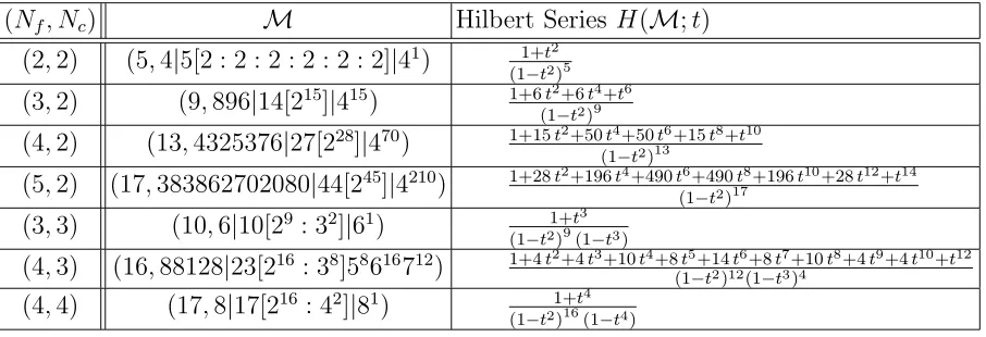
Under our weighting scheme by the R-charge given in (3.23), the moduli space of SQCD, for some low values, is presented in Table 3. There are several agreements, as can be seen from the table. The dimensions do indeed agree with (3.7); moreover, for Nf =Nc,Mis indeed a single hypersurface as can be seen from the defining equations,

in accord with (3.14) and (3.15). Next, we compute the weighted Hilbert series of the second kind and present them to the right of moduli space. The ensuing sections show how these rather complicated rational functions, here found using algorithmic algebraic geometry, can be obtained from the plethystic programme.

(Nf, Nc) M Hilbert Series H(M;t)

(2,2) (5,4|5[2 : 2 : 2 : 2 : 2 : 2]|41₎ 1+t2 (1−t2₎5

(3,2) (9,896|14[215_]|415₎ 1+6t2_+6t4_+t6 (1−t2₎9

(4,2) (13,4325376|27[228_]|470₎ 1+15t2_+50t4_+50t6_+15t8_+t10 (1−t2₎13

(5,2) (17,383862702080|44[245_]|4210₎ 1+28t2_+196t4_+490t6_+490t8_+196t10_+28t12_+t14 (1−t2₎17

(3,3) (10,6|10[29_{: 3}2_]|61₎ 1+t3 (1−t2₎9_(1−t3₎

(4,3) (16,88128|23[216_{: 3}8_]58₆16₇12₎ 1+4t2_+4t3_+10t4_+8t5_+14t6_+8t7_+10t8_+4t9_+4t10_+t12 (1−t2₎12_(1−t3₎4

[image:20.612.86.539.78.233.2]

(4,4) (17,8|17[216_{: 4}2_]|81₎ 1+t4 (1−t2₎16_(1−t4₎

Table 3: _{With natural weighting in (3.23), the vacuum moduli spaceM(Nf,Nc) of SQCD are all}

affine cones over (compact, homogeneous) weighted projective varieties, using notation in (3.24). We also compute the (weighted, second form) Hilbert series. Indeed, forN_f < N_c, M_(Nf,Nc) is triviallyCNf2, with Hilbert series (1−_t2)−Nf2.

number of fundamental fields contained within. Let us return to the unweighted case for a moment. Examining (2.10), we see that the highest power in 1

1−t is the dimension

of M and the coefficient of that leading order term is the degree of M. This is a fundamental property of the Hilbert series of second kind. Now, in the weighted case in Table 3, such a relation persists, and we see immediately that the leading coefficient in the same expansion of the Hilbert series, c, and the degree d of the variety obey the relationcQ

i

wi =d. This is simply the generalisation of the c=d situation of the

unweighted case above.

3.4.4 Further Geometric Properties

As emphasized in the introduction, our technique allows writing down explicit equations for the moduli space. In component form, these equations can be quite complicated. For illustration, we write down M(Nf,Nc); for some low values:

M1,1 = {−y1+y2y3} ;

M2,1 = {−y6y8+y4,−y5y8+y2,−y6y7+y3,−y5y7+y1};

M2,2 = {y2y3−y1y4+y5y6} ;

M3,3 = {y3y5y7−y2y6y7−y3y4y8 +y1y6y8+y2y4y9−y1y5y9+y15y21} .

(3.25)

Observation 3.11. The classical moduli space M(Nf,Nc) of SQCD is irreducible for all value ofNf and Nc.

We conjecture that this is true in general (it should be noted that the algorithms we have employed check this only over the rationals and not over complex coefficient fields). The irreducibility of moduli spaces is certainly not a feature of generic gauge theories; many reducible cases exist in the literature from very early studies of supersymmetric gauge theories. Few recent ones are presented, for example, in [23, 30]. An argument8

why Observation 3.11 may be true in general is that the moduli space as a symplectic quotient (2.4), in the absence of a superpotential is simply C2NcNc_/SL(Nc,C_{). Since} C2NcNc _{is irreducible and SL(Nc,}C_{) is a continuous group, we expect the resulting}

quotient to be also irreducible.

Next, we see that for Nc = 1 (Wess–Zumino model with no continuous gauge

group and 2Nf chiral multiplets), the moduli space is manifestly toric (i.e. generated

as a monomial ideal, consisting of equations of the form ‘monomial = monomial’). This is no surprise, since Nc ≥2 are non-Abelian actions.

Importantly, we can also calculate such familiar quantities, given the defining equa-tion, as the Euler number χ of the compact weighted projective base over which the moduli space is an affine cone. We find that, for example,χ(Base(M2,2)) = 1. Finding

such topological invariants of the moduli space is clearly of great interest and deserves investigation in its own right; we hence leave this to subsequent work. What is per-haps a little surprising is a universal property of the SQCD vacuum: that it is, in fact, Calabi–Yau. We now delve into this fact in the next subsection.

3.4.5 The SQCD Vacuum Is Calabi–Yau

We observe that the numerators of the Hilbert series in Table 3 are palindromic, i.e.

they have the symmetryak =an−k where n is the degree of the numerator and ak are

the coefficients. A rigorous proof of this observation for all Hilbert series of M(Nf,Nc)

using plethystic technique will be given in Section 4.3. There is a beautiful theorem [31], which states:

Theorem 3.12. (Stanley 1978) The numerator to the Hilbert series of a graded Cohen– Macaulay domain R is palindromic if and only if R is Gorenstein.

A similar situation was encountered in [23], and the reader is referred to the discus-sion of Stanley’s theorem there. The point is that our coordinate rings forM(Nf,Nc) are

not merely Cohen–Macaulay9 _{but are algebraically Gorenstein [32]. This is an}

impor-tant conclusion because foraffinevarieties Gorenstein means Calabi–Yau.10_{. Therefore,}

structurally, we conclude that M(Nf,Nc) is, in fact, an affine Calabi–Yau cone over a

weighted projective variety (which itself as a compact space is seen from the above subsections to be rather complicated and not necessarily Calabi–Yau). In brief,

Observation 3.13. The classical moduli space M(Nf,Nc) of SQCD is Calabi–Yau.

3.4.6 The Quantum Moduli Space of SQCD

In this section, we shall summarise the quantum effects on the vacuum moduli space of SQCD. Excellent reviews collecting this work are [1, 5, 6, 7, 33].

3.4.7 The Nf < Nc theories

A non-perturbative Affleck–Dine–Seiberg (ADS) superpotential [1, 5, 6, 7, 33], whose form is consistent with symmetries and holomorphy, is dynamically generated:

WADS =CNc,Nf

Λ3Nc−Nf

detM

1/(Nc−Nf)

, (3.26)

where Λ is the scale of the theory and CNc,Nf is in general renormalisation

scheme-dependent. Because of the dependence ofWADS on meson fields with negative powers,

it is never zero, but flows to zero at infinity. Consequently, at any finite values of the meson fields, WADS is non-zero, and there is no supersymmetric vacuum. Quantum

corrections therefore lead to a ‘runaway’ vacuum.

Although this superpotential is non-polynomial in the quark and antiquark fields, we can still solve for the F-terms and examine the moduli space of solutions, a problem we have adapted to STRINGVACUA [11]. As expected, there is no stable vacuum. The classical vacuum is an auxiliary space that allows for the enumeration of GIOs via the Hilbert series. While the classical vacuum variety does not have a physical meaning in the full quantum theory, it nevertheless encapsulates information about the operatorial structure of SQCD forNf < Nc.

9_{We shall be working with Cohen–Macaulay rings throughout. Briefly, the Cohen–Macaulay}

con-dition for a ringRis that there is a maximalR-regular sequence in the maximal ideal generating an irreducible ideal. This is a technical remark that will not be important to this paper. We have checked this property algorithmically for the cases we have encountered.

10_{For compact, (weighted) projective varieties, this is not enough; Gorenstein means that the}

3.4.8 The Nf ≥Nc theories

The case ofNf =Nc: The moduli space is still parameterised by the basic generators

M, B, and ˜B. The classical constraint (3.14) is however modified by a one instanton effect [1, 5, 6, 7], and the quantum moduli space is described by the relation

det(M)−(∗B)(∗B) = Λe 2Nc . (3.27)

From the constraint (3.14), we see that the classical moduli space is singular at the origin: M = B = ˜B = 0. This singularity does not exist in the true vacuum (3.27), and so the latter geometry is everywhere smooth. Although details of the GIOs and constraints at each order of quarks and antiquarks are modified, their numbers are unaffected. Thus, in spite of different geometrical properties between the classical and quantum moduli spaces, the Hilbert series is not corrected quantum mechanically.

The case of Nf > Nc: In this case, the quantum moduli space coincides with the

classical moduli space [1, 7]. Thus, geometric and algebraic features of the classical vacuum varietyMNf>Nc are also properties of the true vacuum of the theory.

A comment on Seiberg duality: In the conformal window, the convenient

descrip-tion of SQCD may be in terms of dual variables [4]. An early motivadescrip-tion in checking Seiberg duality using Hilbert series is due to Pouliot [24]. Later R¨omelsberger [25] showed that the Hilbert series of SU(2) SQCD with three flavours and its magnetic dual match. There are, however, no further geometric checks in the literature. It is relatively easy to verify that the dimensions of the electric and magnetic theories agree. Using the Hilbert series to more carefully examine the geometric aspects of Seiberg du-ality is clearly an interesting problem that deserves investigation in its own right. We leave this to subsequent work.

4. Counting Gauge Invariants: the Plethystic Programme and

Molien–Weyl formula

Having studied the algebro-geometric properties of the moduli space of SQCD, let us now move on to the problem of enumerating gauge invariants and encoding global sym-metries. There have been a series of works (e.g., [24, 25, 34, 22, 16, 37, 38, 18, 21, 35, 36, 39]) that count the number of BPS GIOs in various gauge theories. However, for SQCD, the computations were usually limited to the caseNc = 2 due to technical

not only a very systematic way of counting the GIOs, but also a deeper understanding of the moduli spaces of SQCD.

In SQCD the chiral GIOs are symmetric functions of quarks and antiquarks which transform respectively in the bifundamental [1,0, . . . ,0; 0, . . . ,0,1] ofSU(Nf)L×SU(Nc)

and the bifundamental [1,0, . . . ,0; 0, . . . ,0,1] ofSU(Nc)×SU(Nf)R. Let us denote the

character of the (anti) fundamental representation of SU(N), respectively, as χSU_[0,...,1](N), and χSU_[1,0,...,0](N) . To write down explicit formulae and for performing computations we need to introduce weights for the different elements in the maximal torus of the dif-ferent groups. We use za, a = 1, . . . , Nc −1 for colour weights and ti,t˜i, i= 1, . . . , Nf

for flavour weights. These weights have the interpretation of chemical potentials11

for the charges they count and the characters of the representations are functions of these variables. Correspondingly, the character for a quark is χSU(Nf_{[1,0,...,0;0,...,0,1]})L×SU(Nc)(ti, za)

and the character for an antiquark isχSU(Nc)_{[1,0,...,0;0,...,0,1]}×SU(Nf)R(za,t˜i). We further introduce two

chemical potentials which count the number of quarks and antiquarks, t, and ˜t, re-spectively. A convenient combinatorial tool which constructs symmetric products of representations is the plethystic exponential, which is a generator for symmetrisa-tion [13, 17, 18, 19, 21]. To briefly remind the reader, the plethystic exponential, P E,

of a function g(t1, . . . , tn) is defined to be exp

_∞ P

k=1 g(tk

1,...,tkn) k

. Whence, we have that

PE htχSU_{[1,0,...,0;0,...,0,1]}(Nf)L×SU(Nc)(ti, za) + ˜tχ

SU(Nc)×SU(Nf)R

[1,0,...,0;0,...,0,1] (za,˜ti)

i ≡ exp " _∞ X k=0 1 k

tkχSU(Nf_{[1,0,...,0;0,...,0,1]})L×SU(Nc)(tk_i, z_ak) + ˜tkχSU(Nc)_{[1,0,...,0;0,...,0,1]}×SU(Nf)R(z_ak,t˜k_i)

#

. (4.1)

A somewhat more explicit form for the character can be

tχSU(Nf_{[1,0,...,0;0,...,0,1]})L×SU(Nc)(ti, za) =χSU[0,...,0,1](Nc)(zl) Nf

X

i=1

ti , (4.2)

which then gives

PE



χSU_[1,0,...,0](Nc)(zl) Nf

X

i=1

˜

ti+χSU(Nc)[0,...,0,1](zl) Nf

X

j=1

tj

 = exp

     ∞ X k=0     

χSU(Nc)_[1,0,...,0](zk l) Nf P i=1 ˜ tk

i +χ SU(Nc) [0,...,0,1](zlk)

PNf j=1tkj

k           . (4.3)

11_{Strictly speaking, they arenot true chemical potentials conjugate to the number of charges. They}

Here, the dummy variables ti and ˜tj are the chemical potentials associated to quarks

and antiquarks counting theU(1)-charges in the maximal torus of the global symmetry. Henceforth, we shall take their values to be such that|ti|<1 for all i.

We emphasize that in order to obtain the generating function that counts gauge invariant quantities, we need to project the representations of the gauge group gener-ated by the plethystic exponential onto the trivial subrepresentation, which consists of the quantities invariant under the action of the gauge group. Using knowledge from representation theory, this can be done by integrating over the whole group (see, e.g., Appendix A of [38] .) Hence, the generating function for the (Nf, Nc) theory is given

by

g(Nf,Nc)=

Z

SU(Nc)

dµSU(Nc)PE



χSU_[1,0,...,0](Nc)(zl) Nf

X

i=1

˜

ti+χSU(Nc)_[0,...,0,1](zl) Nf

X

j=1

tj



 . (4.4)

This formula is also used in the commutative algebra literature (see, e.g., [40]) and is called the Molien–Weyl formula. We note that the Haar measure µSU(Nc) can be

written explicitly using Weyl’s integration formula (see, e.g., Section 26.2 of [41]):

Z

SU(Nc)

dµSU(Nc) =

1 (2πi)Nc−1_N

c!

I

|zl|=1 Nc_Y−1

l=1

dzl

zl

∆(φ)∆(φ−1) , (4.5)

where {φa(z1, . . . , zNc−1)}Nca=1 are coordinates on the maximal torus of SU(Nc) with

QNc

a=1φa= 1, and ∆(φ) =

Q

1≤a<b≤Nc(φa−φb) is the Vandermonde determinant.

Let us take the weights of the fundamental representation of SU(Nc) to be as

follows:

L1 = (1,0, . . . ,0), Lk = (0,0, . . . ,−1,1, . . .0) , LNc = (0, . . . ,−1) , (4.6)

where all L’s are (Nc −1)-tuples, and for Lk (with 2 ≤ k ≤ Nc −1), we have −1 in

the (k −1)-th position and 1 in the k-th position. With this choice of weights, the corresponding coordinates on the maximal torus ofSU(Nc) are

φ1 =z1 , φk=z_k−₋1₁zk , φNc =z−_Nc1₋₁ , (4.7)

where 2≤k≤ Nc−1. Hence, the characters of the fundamental and antifundamental

representations are respectively

χSU_[1,0,...,0](Nc) =

Nc

X

a=1

φa =z1+ Nc_X−1

k=2

zk

zk−1

+ 1 zNc−1

,

χSU_[0,...,0,1](Nc) =

Nc

X

a=1

φ−_a1 = 1 z1

+

Nc_X−1

k=2

zk−1

zk

Putting all the above together, we arrive at the Molien–Weyl formula for computing the generating function for GIOs of SQCD and which also gives an analytic way of computing the Hilbert series for the vacuum moduli spaceM(Nf,Nc):

g(Nf,Nc) = 1 (2πi)Nc−1_N

c!

I

|zl|=1 Nc_Y−1

l=1

dzl

zl

∆(φ)∆(φ−1)× (4.9)

PE

  z1+

Nc_X−1

k=2

zk

zk−1

+ 1 zNc−1

! Nf

X

i=1

˜ ti+

1 z1

+

Nc_X−1

k=2

zk−1

zk

+zNc−1

! Nf X j=1 tj   .

4.1 The Case of Two Colours: Nc = 2

Thus armed, we can compute the generating function for SQCD. Let us begin with two colours where some results are known.

4.1.1 The Example of (Nf = 1, Nc = 2)

There are two chiral multiplets (i.e. a quark and an antiquark being identified) in the theory, and we denote their chemical potentials byt1 andt2. From (4.4), the generating

functiong(Nf=1,Nc=2) _{is given by}

g(1,2)(t1, t2) =

Z

SU(2)

dµSU(2)(z) PE[χSU(2)_[1] (z)(t1+t2)] , (4.10)

whereχSU_[1] (2)(z) =z+ 1/z. Using (4.3), we find that

PE

z+ 1 z

(t1+t2)

= exp 2 X l=1 ∞ X k=1

(ztl)k+ (z−1tl)k

k

!

= 1

(1−t1z)(1−t2z)(1− t_z1)(1−t_z2)

,

(4.11) where we have used the fact that−log(1−x) = P∞

k=1

xk_{/k. Using formula (4.5), we can}

write the Haar measure in (4.10) as

Z

SU(2)

dµSU(2)(z) →

1 2

1 2πi

I

|z|=1

dz z (1−z

2_)(1−z−2_{) . (4.12)}

Therefore we can rewrite (4.9) in the form of Molien integral formula (see,e.g., [24]):

g(1,2)(t1, t2) =

1 2

1 2πi

I

|z|=1

dz (1−z

2_)(1−z−2₎

z(1−t1z)(1−t2z)(1−t1z−1)(1−t2z−1)

. (4.13)

theorem, we find that

g(1,2)(t1, t2) =

1 1−t1t2

=

∞

X

j=0

(t1t2)j . (4.14)

The term t1t2 in the denominator implies that there is only one basic generator of

GIOs which is constructed from two chiral multiplets. Moreover, the series expansion suggests that any other operator in the chiral ring is given as a power of such a basic generator. If we sett1 =t2 =t, then

g(1,2)_{(t) =} 1

1−t2 = 1 +t

2_+t4_+t6_{+. . . , (4.15)}

which is in agreement with the result presented in [24, 21]. Of course, this is also the result for the Hilbert series in Observation 3.2 at Nf = 1, so we have agreement with

the algebro-geometric perspective as well.

4.1.2 (Nf, Nc = 2) with Arbitrary Flavours

Let us move on to the case of arbitrary number Nf of flavours and two colours. Now,

we have 2Nf chiral multiplets. From (4.4), the generating function is then given by

g(Nf,Nc=2)(t1, . . . , t2Nf) =

Z

SU(2)

dµSU(2)(z) PE

 

z+1 z 2Nf X i=1 ti 

 , (4.16)

where, according to (4.3), the plethystic exponential can be written as

exp   ∞ X k=1 2Nf X l=1

(ztl)k+ (z−1tl)k

k  = 2Nf Y l=1

(1−tlz)−1(1−tlz−1)−1 , (4.17)

where again we have used the log expansion. Changing the measure of integration as above, (4.9) becomes

g(Nf,Nc=2)(t1, . . . , t2Nf) =

1 2

1 2πi

I

|z|=1

dz z (1−z

2_)(1−z−2₎ 2Nf

Y

l=1

(1−tlz)−1(1−tlz−1)−1 .

(4.18) The integral can again be evaluated by residues.

For example, in the case Nf = 2, the poles located within the unit circle are

z= 0, t1, . . . , t4 and we find that

g(Nf=2,Nc=2)_(t

1, . . . , t4) =

1−t1t2t3t4

(1−t1t2)(1−t1t3)(1−t1t4)(1−t2t3)(1−t2t4)(1−t3t4)

.

The expressions titj (with 1 ≤ i < j ≤ 4) in the denominator indicate that there are

six basic generators of GIOs, each of which is constructed from two chiral multiplets. Explicitly, these basic generators are mesons. Moreover, the numerator suggests that there is one constraint between these generators at order four of chiral multiplets, namely

PfM =ǫi1...i4M

i1i2_Mi3i4 _{= 0 , (4.20)}

a constraint which has already been seen in (3.17). The general formula for Nf > 1

can be written as

g(Nf>1,Nc=2)(t1, . . . , t2Nf) = 2Nf_P k=1

(−1)k_(t

k)2Nf−3(1−t2k)

Q

1≤i<j≤2Nf i,j6=k

(ti−tj)(1−titj)

2 Q

1≤i<j≤2Nf

(ti−tj)(1−titj)

.

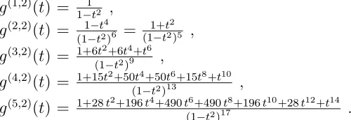
(4.21) Now, if we unrefine and set ti = t for all i= 1, . . . ,2Nf, we should reproduce the

results for the Hilbert series discussed before. Let us present some results for small values of Nf:

g(1,2)_{(t) =} 1 1−t2 ,

g(2,2)_{(t) =} 1−t4

(1−t2₎6 = 1+t 2 (1−t2₎5 ,

g(3,2)_{(t) =} 1+6t2_+6t4_+t6 (1−t2₎9 ,

g(4,2)_{(t) =} 1+15t2_+50t4_+50t6_+15t8_+t10 (1−t2₎13 ,

g(5,2)_{(t) =} 1+28t2_+196t4_+490t6_+490t8_+196t10_+28t12_+t14 (1−t2₎17 .

(4.22)

[image:28.612.181.431.344.430.2]

These highly non-trivial results are in perfect agreement with the right column of Table 3, obtained from a completely different method. We remark that Macaualy 2

[26] can also compute the refined (multi-variate) Hilbert series; we have performed this computation for some examples and the results are exactly as in (4.21). This is encouraging indeed.

In general, the formula g(Nf,Nc=2)_{(t) can be expanded in power series:}

g(Nf,Nc=2)(t) = 1 + 2Nf(2Nf −1)

2 t

2 ₊(2Nf −1)(2Nf)2(2Nf + 1)

12 t

4

+(2Nf −1)(2Nf)

2_(2N

f + 1)2(2Nf + 2)

4(3!)2 t

6_{+. . . . (4.23)}

We can rewrite this equation more compactly, as in (3.18), which in fact holds for all Nf ≥1:

g(Nf,Nc=2)(t) =

∞

X

k=0

(2Nf +k−1)!(2Nf +k−2)!

(2Nf −1)!(2Nf −2)!(k+ 1)!k!

t2k =2F1(2Nf −1,2Nf; 2;t2) .

4.1.3 Plethystic Logarithms and M(Nf,Nc=2)

Recall that according to the plethystic programme the Hilbert series is itself the plethys-tic exponential of a function that encodes the defining relations. This does not contain quite as much information as the defining equations themselves, given in, e.g., (3.25), but it does give the generators and the the relations at each degree. We will thus use theplethystic logarithmto deduce the number of generators and constraints at each order of quarks and antiquarks from the generating function [17, 18]. We recall the expression for the plethystic logarithm,P L, the inverse function toP E, is

PL[g(Nf,Nc)(t)] =

∞

X

k=1

µ(k) k log(g

(Nf,Nc)_(tk_{)) , (4.25)}

where µ(k) is the M¨obius function. The significance of the series expansion of the plethystic logarithm is stated in [17, 18]: the first terms with plus sign give the basic generators while the first terms with the minus sign give the constraints between these basic generators. If the formula (4.25) is an infinite series of terms with plus and minus signs, then the moduli space is not a complete intersection and the constraints in the chiral ring are not trivially generated by relations between the basic generators, but receives stepwise corrections at higher degree. These are the so-calledhigher syzygies.

Let us calculate the plethystic logarithms for Nf = 1, . . . ,4:

PL[g(1,2)_{(t)] = t}2 _,

PL[g(2,2)_{(t)] = 6t}2_−t4 _,

PL[g(3,2)_{(t)] = 15t}2 _−15t4 _{+ 35t}6_−126t8_{+ 504t}10_{+. . . ,}

PL[g(4,2)_{(t)] = 28t}2 _−70t4 _{+ 420t}6_−3360t8_{+ 29148t}10_{+. . . .}

(4.26)

Take PL[g(4,2)_{(t)] as an example: from Observation (3.8), we see that the coefficient}

28 of t2 _{are the number of mesons and the coefficient −70 indicates that there are 70}

constraints among mesons according to (3.17).

We can conclude some properties of the moduli spaces from these results as follows. For (Nf = 1, Nc = 2), there are no constraints between the generators and hence the

moduli spaces arefreely generated. For (Nf = 2, Nc = 2), there are six basic generators

at order two, and one constraint between these generators at order four. Since the dimension of the moduli space (which is dimM(Nf=2,Nc=2) = 22 + 1 = 5) plus the

number of constraints (one) is equal to the number of basic generators (six), the moduli space in this case is acomplete intersection. These conclusions agree with Observations 3.1 and 3.5.

4.2 The Case of Three Colours: Nc = 3

4.2.1 (Nf, Nc = 3) with Arbitrary Flavours

There areNf quarks transforming in the fundamental representation andNf antiquarks

transforming in the antifundamental representation. Using the notation we introduced in (4.4), we find that the generating function is

g(Nf,Nc=3)(t1, . . . , tNf,˜t1, . . . ,˜tNf) =

Z

SU(3)

dµSU(3)PE

 



χSU(3)_[1,0] (z1, z2) Nf

X

i=1

˜

ti+χSU(3)[0,1] (z1, z2) Nf X j=1 tj     , (4.27) withχSU_[1,0](3)(z1, z2) =z1+z_z2₁ +_z1₂, χSU(3)_[0,1] (z1, z2) = _z1₁ +z_z1₂ +z2 and the Haar measure

becomes

R

SU(3)dµSU(3) = 1 6

1 (2πi)2

H

|z1|=1 dz1

z1

H

|z2|=1 dz2

z2 ×

1−z12

z2 1− z2

2 z1

(1−z1z2)

1− z2 z2

1 1−

z1 z2

2 1−

1 z1z2

. (4.28)

The plethystic exponential in (4.27) can be simplified to

Nf

Y

i=1

(1−˜tiz1)(1−˜tiz1−1z2)(1−˜tiz2−1)(1−tiz1−1)(1−tiz1z2−1)(1−tiz2)

−1

. (4.29)

We note that for the z2 integral, the poles inside the unit circle are located at z2 =

0, ˜ti, tiz1, and for thez1 integral, such poles are located atz1 = 0, Qi<j˜ti˜tj, ti. Using

the residue theorem, we find that

g(1,3)(t1,˜t1) =

1 1−t1˜t1

, (4.30)

g(2,3)(t1, t2,˜t1,˜t2) =

1

Q

1≤i,j≤2(1−ti˜tj)

, (4.31)

g(3,3)(t1, t2, t3,t˜1,˜t2,˜t3) =

1−Q3_i=1ti˜ti

(1−Q3_i=1ti)(1−Q3_j=1˜tj)Q_1≤i,j≤3(1−ti˜tj)

. (4.32)

Since the generating function g(4,3) _{in eight variables is very long (three pages in a}

Mathematicanotebook), we shall not present its formula here. However, if we unrefine and setti =t and ˜ti = ˜t, the calculation is slightly easier and we obtain that

g(4,3)_{(t,t) = (1˜ −t}3₎4_(1−t˜t)16_(1−t˜3₎4−1_×

1−4˜t4_{t+ 6˜t}8_t2_−16˜t3_t3_{+ 24˜t}6_t3_−16˜t9_t3_−4˜tt4 _{+ 31˜t}4_t4₋

20˜t7_t4_{+ 10˜t}10_t4_−24˜t8_t5 _{+ 24˜t}3_t6 _−36˜t6_t6_{+ 24˜t}9_t6_{+ 10˜t}12_t6₋

20˜t4_t7_−16˜t7_t7_{+ 24˜t}10_t7 _−16˜t13_t7_{+ 6˜t}2_t8_−24˜t5_t8_{+ 72˜t}8_t8₋

24˜t11t8+ 6˜t14t8−16˜t3t9+ 24˜t6t9−16˜t9t9−20˜t12t9+ 10˜t4t10+ 24˜t7_t10_−36˜t10_t10_{+ 24˜t}13_t10_−24˜t8_t11_{+ 10˜t}6_t12_−20˜t9_t12_{+ 31˜t}12_t12₋

4˜t15_t12_−16˜t7_t13_{+ 24˜t}10_t13_−16˜t13_t13_{+ 6˜t}8_t14_−4˜t12_t15_{+ ˜t}16_t16 _.