Inclusion of coherence in Monte Carlo models for simulation of x-ray phase contrast imaging

Inclusion of coherence in Monte Carlo models

for simulation of x-ray phase contrast imaging

Silvia Cipiccia,1 Fabio A.Vittoria,2 Maria Weikum,1 Alessandro Olivo,2 Dino A. Jaroszynski,1,*

1 _{University of Strathclyde, Department of Physics, Scottish Universities Physics Alliance, John Anderson} Building, 107 Rottenrow, Glasgow, G4 0NG, UK

2 _{Department of Medical Physics and Bioengineering, University College London, Malet Place, Gower Street,} London WC1E 6BT

* dino@phys.strath.ac.uk

Abstract: Interest in phase contrast imaging methods based on electromagnetic wave coherence has increased significantly recently, particularly at X-ray energies. This is giving rise to a demand for effective simulation methods. Coherent imaging approaches are usually based on wave optics, which require significant computational resources, particularly for producing 2D images. Monte Carlo (MC) methods, used to track individual particles/photons for particle physics, are not considered appropriate for describing coherence effects. Previous preliminary work has evaluated the possibility of incorporating coherence in Monte Carlo codes. However, in this paper, we present the implementation of refraction in a model that is based on time of flight calculations and the Huygens-Fresnel principle, which allow reproducing the formation of phase contrast images in partially and fully coherent experimental conditions. The model is implemented in the FLUKA Monte Carlo code and X-ray phase contrast imaging simulations are compared with experiments and wave optics calculations.

References and links

1. B. Lengeler, "Coherence in X-ray physics," Naturwissenschaften 88, 249-260 (2001).

2. A. Bravin, P. Coan, and P. Suortti, "X-ray phase-contrast imaging: from pre-clinical applications towards clinics," Phys Med Biol 58, R1-R35 (2013).

3. T. J. Davis, D. Gao, T. E. Gureyev, A. W. Stevenson, and S. W. Wilkins, "Phase-Contrast Imaging of Weakly Absorbing Materials Using Hard X-Rays," Nature 373, 595-598 (1995).

4. A. Snigirev, I. Snigireva, V. Kohn, S. Kuznetsov, and I. Schelokov, "On the possibilities of x-ray phase contrast microimaging by coherent high-energy synchrotron radiation," Review of Scientific Instruments 66, 5486-5492 (1995).

5. C. David, B. Nohammer, H. H. Solak, and E. Ziegler, "Differential x-ray phase contrast imaging using a shearing interferometer," Appl Phys Lett 81, 3287-3289 (2002).

6. A. Olivo, F. Arfelli, G. Cantatore, R. Longo, R. H. Menk, S. Pani, M. Prest, P. Poropat, L. Rigon, G. Tromba, E. Vallazza, and E. Castelli, "An innovative digital imaging set-up allowing a low-dose approach to phase contrast applications in the medical field," Med Phys 28, 1610-1619 (2001).

7. A. Olivo and R. Speller, "A coded-aperture technique allowing x-ray phase contrast imaging with conventional sources," Appl Phys Lett 91, 074106 (2007).

9. T. E. Gureyev, Y. I. Nesterets, A. W. Stevenson, P. R. Miller, A. Pogany, and S. W. Wilkins, "Some simple rules for contrast, signal-to-noise and resolution in in-line x-ray phase-contrast imaging," Optics Express 16, 3223-3241 (2008).

10. Z. Wang, Z. Huang, L. Zhang, Z. Chen, and K. Kang, "Implement X-ray refraction effect in Geant4 for phase contrast imaging," IEEE Nuclear Science Symposium Conference Record, 2395 - 2398 (2009)

11. A. Prodi, E. Knudsen, P. Willendrup, S. Schmitt, C. Ferrero, R. Feidnhans'l, and K. Lefmann, "A Monte Carlo approach for simulating the propagation of partially coherent x-ray beams," SPIE Advances in Computational Methods for X-ray Optics II, 814108 (2011)

12. E. Bergback Knudsen, A. Prodi, J. Baltser, M. Thomsen, P. Kjaer Willendrup, M. Sanchez del Rio, C. Ferrero, E. Farhi, K. Haldrup, A. Vickery, R. Feidenhans'l, K. Mortensen, M. Meedom Nielsen, H. Friis Poulsen, S. Schmidt, and K. Lefmann, "McXtrace: a Monte Carlo software package for simulating X-ray optics, beamlines and experiments," Journal of Applied Crystallography 46, 679-696 (2013).

13. S. Peter, P. Modregger, M. K. Fix, W. Volken, D. Frei, P. Manser, and M. Stampanoni, "Combining Monte Carlo methods with coherent wave optics for the simulation of phase-sensitive X-ray imaging," Journal of Synchrotron Radiation 21, 613-622 (2014).

14. G. Battistoni, F. Cerutti, A. Fasso, A. Ferrari, S. Muraro, J. Ranft, S. Roesler, and P. R. Sala, "The FLUKA code: description and benchmarking," Hadronic Shower Simulation Workshop 896, 31-49 (2007).

15. F. A. Vittoria, P. C. Diemoz, M. Endrizzi, L. Rigon, F. C. Lopez, D. Dreossi, P. R. T. Munro, and A. Olivo, "Strategies for efficient and fast wave optics simulation of coded-aperture and other x-ray phase-contrast imaging methods," Appl. Opt. 52, 6940-6947 (2013).

16. C. Huygens, Traite' de la lumiere (Leyden, 1690). 17. A. Fresnel, Annales de chimie et physique 28, 147 (1816). 18. E. Hecht, Optics, fourth ed. (Pearson, Harlow, 2003).

19. H. F. Talbot, "Facts relating to optical science", Philosophical Magazine 9, 401-407 (1836).

20. T. Weitkamp, A. Diaz, C. David, F. Pfeiffer, M. Stampanoni, P. Cloetens, and E. Ziegler, "X-ray phase imaging with a grating interferometer," Optics Express 13, 6296-6304 (2005).

21. A. Momose, S. Kawamoto, I. Koyama, Y. Hamaishi, K. Takai, and Y. Suzuki, "Demonstration of X-ray Talbot Interferometry," Japanese Journal of Applied Physics 42, L866-L868 (2003).

22. C. Theis, (personal communication).

1. Introduction

Interest in coherent X-ray imaging has grown substantially over recent years[1] and X-ray phase contrast imaging (XPCI) is one of the most promising methods. X-ray absorption imaging is not suitable for weakly absorbing material, where the contrast is significantly impaired [2]. XPCI, which is based on the phase shift introduced by the object, provides a way of overcoming this limit. Different techniques have been developed for XPCI, most of which require highly coherent sources, e.g. analyser based imaging (ABI) [3], which requires low transverse coherence but high temporal coherence, or in-line holography [4] and grating interferometry [5], both of which require the contrary. To date, the only XPCI method that requires neither spatial nor temporal coherence is edge illumination (EI) XPCI [6, 7].

A suitable starting point for describing the formation of a phase contrast image is provided by the Fresnel-Kirchoff diffraction theory. However, in conditions of limited coherence, a simpler ray-tracing approach can also be used. Peterzol et al. [8] have shown that the two approaches are equivalent when the following condition is satisfied:

1 2 1, 2 _g

r M

F

 

 

 

(1)

where  is the x-ray wavelength, r1 is the object to detector distance, M is the system

between the detector point spread function (PSF, response of the detector to a point source) and the projected source distribution, i.e. source distribution multiplied by the sample-to-detector and divided by the source-to-sample distance.

While simplified expressions exist [9], rigorous approaches for coherent sources typically require the solution of Fresnel-Kirchhoff diffraction integrals. These have to be solved numerically and can be very computationally-intensive, particularly for two-dimensional images. A major limitation of the wave optical approach is that the wave front must be stored in numerical calculations, which limits the domain size. A Monte Carlo approach could provide an alternative to wave optics calculations because, despite being computationally intense, the wavefront does not need to be stored. Moreover it is highly parallelizable, which enables larger size simulations to reproduce complex object geometry and source properties. Coherent Monte Carlo simulations may represent a useful tool for experiment planning and data interpretation.

Previous studies have described the possibility of implementing a ray tracing approach in a Monte Carlo code [10]. More recently, preliminary studies on ways of including coherent propagation and diffraction based on Huygens-Fresnel principle have been presented [11, 12]. A combination of ray-tracing and wave optics with the reconstruction of the phase from the path length [13] has also been proposed to reproduce XPCI patterns. However, because these are based on ray tracing, its application is limited to cases where the condition given by Peterzol [8] is satisfied. In this paper, we discuss the implementation of the Huygens-Fresnel principle in the FLUKA Monte Carlo code for the first time including refraction. We first show a simple implementation of refraction via ray-tracing in FLUKA, and then include a wave-optics equivalent approach. To validate the method we show that this correctly reproduces XPCI images produced using various approaches, including free space propagation (FSP), edge illumination (EI) and Talbot interferometry. We compare the simulations results with experimental measurements and wave-optical modelling. Finally, we note that the proposed approach is sufficiently general to be implemented in any Monte Carlo code.

2. Ray-tracing approach

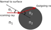
Before implementing coherence effects through inclusion of the Huygens-Fresnel principle, we tackle the simpler problem of describing XPCI under relaxed coherent conditions (as defined in Peterzol et al. 2005 [8]) through a simplified ray-optics approach. The inclusion of Snell’s law in a Monte Carlo code only requires knowledge of the refractive index of the simulated materials. The direction of the particle entering or exiting the refractive object is rotated about the normal to the surface of an angle  = 2 - 1, where 1(2) is the angle

between the incoming (outgoing) ray, and the perpendicular to the plane defined by the incoming ray and the normal to the surface passing for the boundary crossing point (see Fig. 1). 1 and 2 satisfy Snell’s law

1 2

2 1

s in ( )

,

s in ( )

n n    

 (2)

where





1 2 1 1 2

n 

   represent the real parts of the complex refractive index of the two

media.

position coordinates and direction cosines of the particle as it crosses the boundary between two regions. The distribution of photons on a downstream screen is recorded.

Fig. 1. Schematic of the ray-tracing approach for phase contrast imaging.

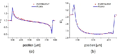
To verify the validity of the ray-tracing implementation in FLUKA, the results are compared with two experiments and wave-optical calculations for FSP (using the code described by Vittoria et al., 2013[15]). In the first case, a 78 m radius polyetheretherketone (PEEK) wire is immersed in 5 mm of water and imaged with a 9.7 keV X-ray beam using a CCD camera with an image relay that gives an effective pixel size of 0.8 m (Fg was 15 m). The source-sample distance is 220 m and the source-sample-detector distance is 0.58 m. For the second, a 100

m nylon wire is imaged with Fg of 140 m at 20 keV. The source- to-sample distance is 25 m and the sample-to-detector distance 1.4 m. The results are shown in Fig. 2.

Fig. 2. Comparison of FLUKA simulations with experimental data. Red dots: experimental data: a) PEEK wire in water: PEEK = 2.98 × 10-6, WATER = 2.46 ×

10-6. b) nylon wire: NYLON = 5.53 × 10-7. For both simulations the number of

particles simulated is 5 x 108_{, the computational time per particle is ~1 x 10}-6 _s.

3. Wave-optical approach

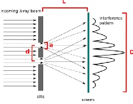
FLUKA usually treats photons as particles and their wave nature is not implemented. It therefore cannot reproduce diffraction and interference phenomena. However, this can be implemented by including the Huygens-Fresnel principle [16, 17], where each point of a wave front is a source of secondary spherical waves, and their subsequent interference forms the next wave front. For example, to reproduce the interference in a double slit experiment, when a photon crosses a slit aperture its direction cosines are diffracted at an angle D following an isotropic probability distribution (see Fig. 3). The obliquity factor   1 c o s / 2

D D

K    

[18], which takes into account the directionality of the secondary emission, can be assumed to be 1 for small diffraction angle, a condition that is satisfied if D /L 1, where D is the screen width and L the slit-detector distance. When a photon hits the detector, the energy (E), time of flight (tof) and position are recorded. Using a post-processing code written in MATLAB, photons arriving at the detector screen are binned, and in each bin each photon is

assigned a phasor o f, E i t

e

modulus of the sum of the phasors    

2 2

i i

i i

I  _   _ _   _







. The intensity

distribution on the screen obtained in this way reproduces the expected interference pattern. To verify the validity of the above approach, a double slit experiment has been simulated using FLUKA.

Fig. 3. Double slit setup simulated in FLUKA. d is the slit distance, a the slit width. The photons after the slits are scattered isotropically within an angle ±D/L.

The expected interference pattern for a two slits experiment is given by

   

2 2 s in c o s

m

I  I  



 

 _{ }

  [18], where Im is the intensity at the centre of the pattern,

s i n ,

a



 



  _d /_, a is the slit width, d is the distance between the slits,  the

angle from the central axis and  the x-ray wavelength. The description holds when 2

d L



(far-field). A comparison between an analytic and simulated interference pattern is shown in Fig. 4. The good agreement gives confidence in the validity of the approach to reproduce diffraction.

Fig. 4. Double slit experiment. The analytic interference pattern (black dotted line) is compared with that produced using FLUKA (blue solid line) for a 20 keV X-ray beam transmitted through two slits with a = 5 m d = 35 m and L = 20 m. Number of simulated particle 2 x 108_{, processing time 1.2 x 10}-5 _{s per}

particle.

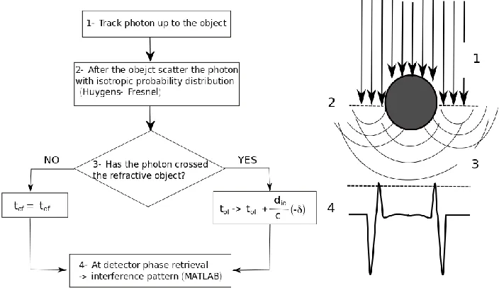
passing through and outside the object. Moreover, the time of flight of each photon reaching the detector screen is corrected to take account of refraction as follows:

 ,

io o f o f

d

t t

c



   (3)

where dio is the photon path length inside the refracting object and  is the real part of the refractive index. It is worthwhile noting that if the photon does not pass through the object, the corrected time of flight corresponds to the time of flight given by FLUKA. The details of the implementation in FLUKA of the time of flight corrections can be found in the Appendix. As in the case of the double slit experiment, photon position, corrected time of flight and energy when reaching the detector screen are recorded, and the intensity is calculated in each bin at the end of the simulation to reconstruct the interference pattern (Fig. 5).

Fig. 5. (a) Flow chart summarizing the steps to implement refraction in FLUKA. (b) Illustration of photon propagation in FLUKA corresponding to the steps in the flow chart.

Fig. 6 shows that the interference patterns obtained with FLUKA are in good agreement with classical wave-optical calculations [15] for 50 m radius PEEK (low absorption) and tungsten (high absorption) wires for 20 keV X-rays, a 1 m sample-to-detector distance and idealized conditions where Fg = 0.

4. Beyond Free Space propagation: Edge Illumination

The ray-tracing and wave-optical approaches implemented in FLUKA can be used to simulate any phase contrast imaging technique. As an example, we have simulated an EI XPCI experiment using the ray-optical approach. The image formation principle in EI is based on intercepting one or more shaped beams through an absorbing edge: sample- induced refraction will then produce a modulation in the signal detected by the pixels (Fig. 7).

Below we compare the phase contrast image PEEK and Titanium wires of a 232 m and 125

m radius respectively performed with 20 keV x-rays, Fg = 80 m, source-to-sample distance

by 10 m, resulting in a 50% illumination fraction. Details of the experimental setup can be found in Olivo et al., 2001 [6]. The results are presented in Fig. 8.

Fig. 6. Wave-optical approach interference pattern obtained using FLUKA (blue line) and by numerically solving the Fresnel/Kirchhoff integral (black line) using 20 keV monochromatic X-rays to image 50 m radius PEEK wire, PEEK

= 7.15 × 10-7 _{(a) and 50 m tungsten wire, }

W = 8.03 × 10-6 (b). The number of

simulated particles is 1x109_{, processing time 0.8 x 10}-5 _{s per particle.}

Fig. 7. Edge-illumination XPCI (not to scale). The figure extends in the plane of the drawing sufficiently to laterally cover the full sample, which is scanned along one direction only. With non-laminar (e.g. cone) beams, multiple beams are created through masks and scanning is avoided.

Fig. 8. EIXPCI experiment: a) PEEK wire profile,  PEEK = 7.15 × 10-7 and b)

titanium wire profile,  TITANIUM = 21.9 × 10-7. The experimental step size is 10

m, the simulated scanning step 1m. The figures show FLUKA results compared to the experimental data. The simulated number of particle is 5 x 107

5. Talbot interferometer

To demonstrate the effectiveness of the wave-optical approach implemented in FLUKA including the Huygens-Fresnel principle, we have simulated image formation in a Talbot interferometer, i.e. an x-ray imaging technique based on a purely coherent effect [19]. When a coherent, plane monochromatic wave is incident on a periodic grating, the image of the grating (self-image) is repeated at periodic distances known as Talbot distances. The use of the Talbot interferometer as an imaging device has been extensively studied and detailed description can be found in the literature [20, 21]. Very briefly, the Talbot interferometer is based on two gratings: a phase grating and an absorption grating. The absorption grating is placed at a longitudinal distance from the phase grating corresponding to the Talbot distance. A transverse scan of the absorption grating makes possible to record the intensity modulation due to the self image. If a refractive object is placed before the phase grating, the self image is distorted. From the comparison of the intensity modulation with and without object, the phase shift induced by the object can be retrieved. In our simulation, a 250 m radius PEEK wire is illuminated by a 20 keV X-ray beam. Both the phase and the absorption grating have a pitch of m and a 50% open fraction. The absorption grating is placed at half the Talbot distance, where the self-image should appear shifted by half the pitch. The presence of a refractive object distorts the self image. The phase shift is measured by scanning the second grating in 30 steps of 0.2 m (Fig. 9). From the phase shift (Fig. 10(a)) in each pixel, the phase shift induced by the object is reconstructed (Fig. 10(b)).

Fig. 9. Schematic of the Talbot interferometer implemented in FLUKA. The distance between the phase and the absorption gratings is 12.5 cm, corresponding to half the first Talbot distance.

6. Conclusion

In the paper we have described a method of including coherence effects for phase contrast imaging in the Monte Carlo code FLUKA. The approach is sufficiently general to be easily imp0lemented in other Monte Carlo codes.

To validate this approach, we have demonstrated phase contrast techniques and reproduced both ray-tracing and wave optical approaches, which compare extremely well with experiments.

The geometry chosen to validate the proposed approach is a very simple 1D geometry (wire). In general, for very simple geometries, solving the Fresnel/Kirchoff integral is faster than the Monte Carlo approach. However, it is in implementing very complex geometries and sources that the advantages of using a Monte Carlo approach become apparent, thanks to the capability of interfacing with existing geometry software for an easier inclusion of geometrical characteristics of the imaging system and high parallelizability. To allow the reader to compare the computational time of the proposed approach with other methods (Monte Carlo and not only), the resources used for the simulations (see Appendix) and the average computational time per particle have been given for each simulation.

The implementation can be pushed further to include polarization effects. Moreover, variations in statistical photon noise caused by the object and large-angle scattering events can both be included in a Monte Carlo approach, and also situations which, for example, fall outside the paraxial approximation could be investigated.

7. Appendix

All the FLUKA simulations presented in this paper have been run on a single processor Intel® CoreTM i7-3740QM, 2.7 GHz. of a DELL Precision M4700.

The number of simulated particles has been set on a case-by-case basis, to reach a steady state in the results. Before this steady state is reached, the relative amplitude of the interference pattern increases with an increase in the number of simulated particles.

In FLUKA simulations, the reading and writing of the direction cosines of the photons while crossing boundaries between two regions are implemented in the user subroutine USRMED. The direction cosines of the normal to the surface at the crossing point are returned by FLUKA by calling the subroutine GEONOR _ENREF_19[22]. The energy, position and time of flight of the photons at the detector screen have been recorded implementing the user subroutine MGDRAW. The correction of the time of flight is implemented inside the customized user subroutine MGDRAW via the entry BXDRAW. BXDRAW is called when a particle crosses two different regions, and the entry gives access in reading mode only to the position, momentum, direction cosines of the particle at the crossing point. If the particle enters the refractive object, its entrance coordinates are saved. If the same particle exits the refraction object, the path length inside the object is calculated from the exit coordinates and the previously saved entrance coordinates, the path length inside the object is calculated. Knowing the refractive index of the object, the time of flight is then calculated using the formula in section 3, and written to an output file. The post-processing of FLUKA output files has been done using a MATLAB code.

Acknowledgments