Quantitative single shot and spatially resolved plasma wakefield diagnostics

Quantitative single shot and spatially resolved plasma wakefield diagnostics

Naren Ratan,2 James Sadler,2Robert Bingham,3,5Philip N. Burrows,1 Raoul Trines,3 Matthew Wing,4 and Peter Norreys2,3

1

John Adams Institute, Denys Wilkinson Building, Keble Road, Oxford OX1 3RH, United Kingdom 2

Clarendon Laboratory, Department of Physics, University of Oxford, Parks Road, Oxford OX1 3PU, United Kingdom

3

STFC Rutherford Appleton Laboratory, Chilton, Didcot OX11 0QX, United Kingdom 4

Department of Physics and Astronomy, University College London, Gower Street, London WC1E 6BT, United Kingdom 5

Department of Physics, University of Strathclyde, Glasgow G4 0NG, United Kingdom (Received 5 May 2015; published 6 August 2015)

Diagnosing plasma conditions can give great advantages in optimizing plasma wakefield accelerator experiments. One possible method is that of photon acceleration. By propagating a laser probe pulse through a plasma wakefield and extracting the imposed frequency modulation, one can obtain an image of the density modulation of the wakefield. In order to diagnose the wakefield parameters at a chosen point in the plasma, the probe pulse crosses the plasma at oblique angles relative to the wakefield. In this paper, mathematical expressions relating the frequency modulation of the laser pulse and the wakefield density profile of the plasma for oblique crossing angles are derived. Multidimensional particle-in-cell simulation results presented in this paper confirm that the frequency modulation profiles and the density modulation profiles agree to within 10%. Limitations to the accuracy of the measurement are discussed in this paper. This technique opens new possibilities to quantitatively diagnose the plasma wakefield density at known positions within the plasma column.

DOI:10.1103/PhysRevSTAB.18.081302 PACS numbers: 42.25.Dd, 52.35.Mw, 52.38.Kd, 42.62.Eh

I. INTRODUCTION

When a driver is fired into an underdense plasma, it will generate a large amplitude longitudinal wave in the electron density profile, now widely known as a plasma wakefield

[1–3]. Due to gradients in the electron density profile, the driver beams induce electric fields up to tens or hundreds of GV/m[4–7]. This is three orders of magnitude higher than the electric field produced in conventional accelerators.

If the wakefield is driven by a short laser pulse[8,9], a beat wave[10–12], an electron[13–15], or a proton beam

[16,17], all of which propagate with speeds near the speed of light in vacuum, the wakefield also propagates with approximately the same speed as the driver. The large accelerating gradient and high propagation speed of the wakefield makes it possible to use plasma as a basis for a particle accelerator[18–20].

Before 2006, the core part of a plasma accelerator, i.e., the wakefield structure itself, had never been imaged in experiments. The first snapshot of the wakefield was taken using the frequency domain holography method [21]. It used two long chirped pulses to copropagate with the

wakefield, as demonstrated in Refs. [22–25]. The phase modulation of the pulse was retrieved from a spectrometer. From the phase modulation profile, the image of a plasma wakefield was obtained. This major advance in diagnostic development has since allowed much greater understanding of the underlying physics. However, one limitation is that the probe pulse copropagates with the wakefield, and so there is an averaging effect of the retrieved wakefield profile. Therefore, it is not possible to diagnose the evolution of the wakefield along the propagation direction. In 2014, the same group demonstrated a new plasma wakefield diagnostic technique which used two long chirped pulses fired at a certain angle relative to the laser pump pulse [25], which is called the frequency domain streak camera. By measuring the phase modulation of the probe pulse, this technique successfully produced the longitudinal evolution of a wakefield in a single shot. It is useful to detect where the bubble in the wakefield is formed. However, the transverse structure of the wakefield is convolved in the probe’s phase modulation. Because this technique does not provide the transverse structure infor-mation, there is insufficient information in the data pro-duced in this technique to quantify the wakefield density modulation.

In other experiments, images of plasma wakefields were obtained using shadowgraphy technique[26,27]. In these elegant experiments, probe laser pulses were fired across Published by the American Physical Society under the terms of

the wakefield in the perpendicular direction. The transverse intensity profiles of the probe pulses represented the second derivative of the wakefields’electron density profiles with respect to position. This allowed the crossing point to be chosen along the propagation distance of the driver. However, because the plasma wakefield propagates with a speed near the speed of light in vacuum, the relative longitudinal position of the probe changes while it is still interacting with the wakefield. This makes it quite difficult to obtain quantitative data from this technique.

In this paper, a novel technique to image and diagnose plasma wakefields, using the concept of photon acceler-ation, is presented. When photons propagate in a plasma wakefield, their frequencies change according to the gradient of the wakefield’s density profile relative to the photons’ positions. This phenomenon was first predicted by Wilkset al.[28]and further developed in Refs.[29–32]. By measuring the frequency modulation of the photons, one can retrieve the electron density modulation profile in the wakefield.

In a previous study[33], pioneering results of simulated measurements using photon acceleration using a long copropagating probe pulse were presented. As in frequency domain holography, the setup introduces an averaging effect, which was accounted for in the description of its strengths and limitations. In order to avoid the averaging effect, a new study is presented here where the probe pulse is allowed to propagate with an oblique angle relative to the wakefield. This oblique crossing angle makes it possible to obtain the density modulation profile of the wakefield at certain positions and diagnose the evolution of the wake-field along the propagation distance, thereby overcoming one of the limitations of the previous methods. This technique is also complementary to the frequency domain streak camera technique[25]by providing the quantitative information of the electron density modulation in the wakefield.

If the angle is set correctly, the velocity of the probe pulse in the wakefield’s longitudinal direction is the same as the wakefield’s group velocity and the longitudinal position of the probe pulse will not change relative to the wakefield. Therefore, an inverse Abel transform [34]

can be applied, with the assumption that the wakefield has a cylindrical symmetry. However, the correct angle is not always achievable, especially for the case where the wakefield’s speed is greater than the probe’s speed. For different crossing angles, the probe pulse’s relative longi-tudinal position changes while crossing the wakefield and an ordinary Abel transform cannot be applied.

In this paper, an expression of a modified Abel transform is derived so that it can be applied for more general crossing angles with its inverse transformation. Results of the simulated measurements are presented for various wake-field amplitudes, frequencies of the probe beam, and crossing angles. In the simulations, two electron density

profiles of the wakefield were obtained. The first were obtained directly from the electron density profiles in the simulations, and these are called“actual”profiles through-out this paper. The second were calculated from the electric field profiles of the laser pulse in the simulations. These profiles are called“measured”profiles. The“actual” and “measured” terms will be used often in this paper. These two types of profiles are then compared to confirm the agreement between them. Analysis of the limiting conditions, including the diffraction effect and error-dependence on the angle of incidence, are also discussed. This paper is organized as follows. In Sec.II, a derivation of a transformation for cylindrically symmetric objects with oblique crossing angle is derived. The simulations’ param-eters are presented in Sec. III. Section IV provides the results of the simulations and discussions of the results and the limiting conditions. Finally, in Sec.V, conclusions of this paper are presented.

II. THEORETICAL ANALYSIS A. Forward transform

It is well known that if a photon propagates through a medium with varying refractive index in space, the wave-length of the photon changes while its frequency remains constant. This does not happen if the medium is moving. In this case, the refractive index of the medium varies in both space and time. Thus, it changes the frequency and wave-length of photons that propagate in it.

When a plasma wakefield is generated in a plasma, the electron density variation gives different refractive indices at every position and time. If a laser pulse propagates in the wakefield, the frequency is shifted by the amount[29,32]

Δω ω0 ≈ −

ω2_p

2ω2 0

c n₀

Z _∞

−∞ ∂n

∂ζdt ð1Þ

By taking t¼0 when the photon is closest to the wakefield’s axis, the position of the photon in the wakefield in cylindrical coordinates is

rðtÞ ¼ ½ðvgtsinθÞ2þy21=2; xðtÞ ¼v_gtsinθ;

ζðtÞ ¼ζ0þ ðvgcosθ−upÞt; ð2Þ

whererðtÞdenotes the distance from the wakefield’s axis,y is the shortest distance from the axis, andζ₀represents the probe’s longitudinal position when it is at the shortest distance from the axis.

In this case, the wakefield density profile is assumed to have a cylindrical symmetry. By defining fðr;ζÞ≡

ð−ω2

pc=2ω20n0Þð∂n=∂ζÞ and Fðy;ζ0Þ≡ðΔω=ω0ÞðvgsinθÞ, Eq. (1)can be written as

Fðy;ζ0Þ ¼vgsinθ Z _∞

−∞f½rðtÞ;ζðtÞdt: ð3Þ

Using Eq. (2) and expanding f½rðtÞ;ζðtÞ around ζ¼ζ₀ using Taylor’s series, the function can be written as

f½rðtÞ;ζðtÞ ¼X∞

j¼0

∂j_f

∂ζj½rðtÞ;ζ0

½ðv_gcosθ−u_pÞtj j! : ð4Þ

Substituting fðr;ζÞ from Eq. (4) to Eq. (3) and t¼ x=v_gsinθfrom Eq. (2)yields

Fðy;ζ0Þ ¼

X∞

j¼0

aj j!

Z _∞

−∞ ∂j_f

∂ζjðr;ζ0Þxjdx ð5Þ

wherea≡½ðcosθ−u_p=v_gÞ=sinθindicates how much the photon shifts horizontally relative to the wakefield.

The integration in Eq.(5)is an integration forxwhile the functionfis expressed inr. From Eq.(2), variablexcan be substituted asx¼ pffiffiffiffiffiffiffiffiffiffiffiffiffiffir2−y2. Thesign onxallows the integral to be split into two parts. The first integrates from r¼∞tor¼yfor negativexand the second fromr¼yto r¼∞ for positivex. Odd values ofjmake the integrand signs for negativex and positive xthe same. It therefore follows that the integrations for negative x cancel the integrations for positivexfor odd values ofj. It is important to note that this is not the case for even values ofj, because the integrations for negative and positivexhave the same values. Rewriting Eq.(5)in terms of r gives

Fðy;ζ0Þ ¼2

X∞

j¼0

a2j

ð2jÞ! Z _∞

y ∂2j_f ∂ζ2jðr;ζ0Þ

ðr2_−y2_Þj ffiffiffiffiffiffiffiffiffiffiffiffiffiffi r2_−y2

p rdr:

ð6Þ

This allows Eq. (6) to be calculated for known distri-butions offðr;ζÞ. Further simplification can be made using a pseudodifferential operator with a Fourier transform[35]. One property of a Fourier transform is that one can transform ∂jf=∂ζj into ðikÞjf~ where the tilde represents the Fourier transform off, i.e.,f~ðr;kÞ ¼R_−∞∞ fðr;ζÞe−ikζdζ. By applying a Fourier transform onfðr;ζÞandFðy;ζ₀Þin both theζ and ζ₀ directions, Eq.(6) is rewritten as

~

Fðy; kÞ ¼2 Z _∞

y X∞

j¼0 ð−1Þj

ð2jÞ!

kaqffiffiffiffiffiffiffiffiffiffiffiffiffiffir2_−y2

_2j~

fðr; kÞrdr ffiffiffiffiffiffiffiffiffiffiffiffiffiffi r2_−y2

p :

ð7Þ

The variableF~ðy; kÞrepresents the Fourier transformation ofFðy;ζ₀Þ, or F~ðy; kÞ ¼R_−∞∞ Fðy;ζ₀Þe−ikζ0_dζ

0.

The Taylor’s series of a cosine function is cosx¼P∞_j¼0ð−1Þjx2j=ð2jÞ!, so the series terms in Eq.(7)

can be substituted by a cosine function. Thus, the equation can be simplified as

~

Fðy; kÞ ¼2 Z _∞

y cos

kaqffiffiffiffiffiffiffiffiffiffiffiffiffiffir2_−y2

rf~ðr; kÞ

ffiffiffiffiffiffiffiffiffiffiffiffiffiffi r2_−y2

p dr: ð8Þ

This expression is similar to an Abel transformation

[36–38] except that it contains a cosine factor in the integral. The zero value of the variable a turns Eq. (8)

into an Abel transform. It represents the special case where the probe pulse propagates perpendicularly relative to the wakefield.

To obtain Fðy;ζ₀Þ, Eq.(8)is simply transformed using the inverse Fourier transform. Most importantly, the equa-tion applies for any case where measurements are made in FIG. 1. The configuration considered in this paper: the laser

cylindrically symmetric objects using nonperpendicular probes.

B. Inverse transform

When performing the measurement, one is mostly interested in obtaining the profile of fðr;ζÞ. To do this, one first measuresFðy;ζ₀Þand then one inverts it using the inverse transform of Eq. (8). This is

~

fðr; kÞ ¼−1

π

Z _∞

r ∂F~ ∂yðy; kÞ

coshðkapffiffiffiffiffiffiffiffiffiffiffiffiffiffiy2−r2Þ ffiffiffiffiffiffiffiffiffiffiffiffiffiffi y2_−r2

p dy: ð9Þ

To verify Eq.(9), it is easier to start from Eq. (8) and rewrite it in the form of

~

Fðy; kÞ ¼−2 Z _∞

y

sinðkapffiffiffiffiffiffiffiffiffiffiffiffiffiffir2−y2Þ ka

∂f~ðr; kÞ

∂r dr ð10Þ

by using partial integration and assuming that limr→∞rf~ðr; kÞ ¼0. Then taking the y-derivative of Eq. (10)yields

∂F~ðy; kÞ

∂y ¼2y Z _∞

y

∂f~ðs; kÞ

∂s

cosðkapffiffiffiffiffiffiffiffiffiffiffiffiffiffis2−y2Þ ffiffiffiffiffiffiffiffiffiffiffiffiffiffi s2_−y2

p ds: ð11Þ

Substituting Eq. (11)into Eq. (9)gives

~

fðr; kÞ ¼−2_π Z _∞

y¼ry Z _∞

s¼y

∂f~ðs; kÞ

∂s

cosðkapffiffiffiffiffiffiffiffiffiffiffiffiffiffis2−y2Þ ffiffiffiffiffiffiffiffiffiffiffiffiffiffi s2_−y2

p

×coshðka

ffiffiffiffiffiffiffiffiffiffiffiffiffiffi y2_−r2

p

Þ

ffiffiffiffiffiffiffiffiffiffiffiffiffiffi y2_−r2

p dsdy:

Then by changing the order of integration, one obtains

~

fðr; kÞ ¼−2

π

Z _∞

s¼r

∂f~ðs; kÞ

∂s

× Z _s

y¼ry

cosðkapffiffiffiffiffiffiffiffiffiffiffiffiffiffis2−y2Þcoshðkapffiffiffiffiffiffiffiffiffiffiffiffiffiffiy2−r2Þ ffiffiffiffiffiffiffiffiffiffiffiffiffiffi

s2_−y2

p ffiffiffiffiffiffiffiffiffiffiffiffiffiffi y2_−r2

p

× dyds: ð12Þ

It can be shown that they-integration on Eq.(12)isπ=2and does not depend ons,r,k, anda(see AppendixA). Thus, from Eq.(12), one can write

~

fðr; kÞ ¼−2

π

Z _∞

s¼r

∂f~ðs; kÞ

∂s π

2ds¼f~ðr; kÞ; ð13Þ

which confirms that Eq. (9)is the inverse of Eq. (8). The inverse transformation in Eq. (9) can be imple-mented using 3-points Abel transformation with some

modifications [39]. Details of the implementation tech-nique are given in AppendixB.

III. SIMULATION PARAMETERS

Simulations using the OSIRIS 3D code [40–42] were

performed.OSIRISis a fully relativistic particle-in-cell code

that can simulate plasma and electromagnetic waves and has been extensively benchmarked against experiments in laser plasma accelerators over the past two decades.

These simulations were performed to model realistic conditions expected in experiments and to check the accuracy of the measurements. In the baseline parameters of the three dimensional simulations, a cold plasma was used with a density ofn₀¼2×1019 cm−3. The simulation window contains9750×400×300cells each with size of

ð12×120×120Þnm3. One particle per cell was used and this was found to be sufficient for these purposes (the simulations were repeated using a larger number of particles per cell and gave similar results). A moving window simulation was deployed. Periodic boundary con-ditions were used in the transverse direction.

The driver of the wakefield was an electron beam which had a spherical Gaussian shape withσr¼4.4μm and peak density of ne ¼0.33n0 to drive the wakefield amplitude

around∼0.53n₀. Each of the electrons in the driver beam propagated with momentum ofp=mec¼45×103, where me was the mass of an electron. The probe pulse was a plane wave with wavelength of 400 nm, duration of 53 fs and normalized intensity ofa₀¼0.01. The probe crossed the wakefield with an angle ofθ¼20o_{. In the simulation,}

5 slices of the probe pulse were taken. The slices crossed the center of the wakefield at the propagation distance of s¼28;39;49;60, and 67μm after the driver entered the plasma. These parameters were chosen to minimize the computational cost of the simulations. Each simulation took around 8000 CPU hours to finish in average. Figure2

illustrates the simulation and slicing of the electric field, taken from the actual results of the simulation.

To determine the accuracy of the measurement over some parameters, the density of the driver beam was varied from0.1n₀to0.35n₀, the crossing angle from 25° down to 5°, and the probe’s wavelength from 260 to 800 nm.

“measured”profiles. The actual and the measured density modulation profiles are compared to see how well those values agree.

To extract the frequency profile of the laser probe pulse in the simulation, a Wigner transform was used, as described in Ref.[33]. This gives flexibility in the choice of 2D phase or frequency extraction methods in real experiments. These include single-shot supercontinuum spectral interferometry[21,22,25], frequency domain inter-ferometry[43,44], SPIDER[45], etc. Therefore, analysis of the accuracy and precision in real experiments need to be combined with error analysis from the chosen method.

IV. RESULTS AND DISCUSSION A. Results of measurement simulations

In the simulations, the wakefield amplitude did not significantly change during the interaction with the probe pulse. Also, the amplitude of frequency modulation of the laser pulse is not significantly different between the slices FIG. 2. Illustration of the simulation, taken from the actual

results of the simulation. The left picture show the sliced wakefield in the electron density profile at x₃¼0. The right picture illustrates the initial electric field profile of the probe pulse. The red line on the right picture shows one of five planes where the slice of the electric field crosses the wakefield at the propagation distance s¼28μm after the driver entered the plasma. The axesx₁,x₂, andx₃ in this illustration are different from the axes x, y, z in the previous figure where in this illustration the laser probe pulse propagate parallel withx₁-axis. While in Fig. 1, the probe pulse propagates not parallel to any axis.

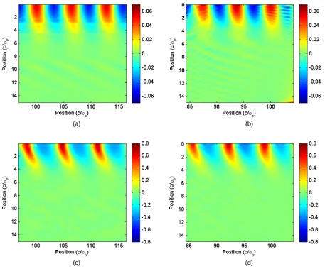
taken along the plasma column. The 2D frequency profile of the slice of the laser pulse that crosses the center of the wakefield at s¼28μm was obtained shortly after it had interacted with the wakefield for the cases of small and large wakefield amplitudes. Figure3shows the comparison between the measured electron density modulation profiles from the laser pulse and the actual density modulation profiles for both cases.

As seen in Fig.3, the measured electron density profiles share similar shapes with the actual density profiles shortly after the probe pulse crosses the wakefield. However, as the pulse propagates, the measured density profile from the probe pulse changes its shape. The amplitude of the modulation also decreases, as seen in Fig. 4. Therefore, measuring the density profile after the laser pulse prop-agates some distance could lead to inaccurate measure-ments. This is an unwanted diffraction effect and can be mitigated in real experiments using 4f image relaying setups [46]. Another unwanted effect is dispersion which can be eluded by avoiding transmissive optics in the experiment.

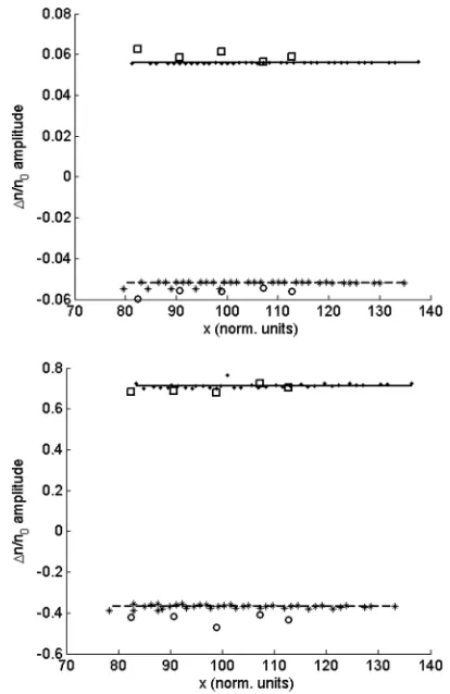
Before the diffraction effect on the measured profile becomes significant, a comparison was made between the peaks and troughs values of the measured and actual density modulation profiles. Figure5shows the peaks and troughs values of the actual and measured density modulation profiles from 5 slices along the plasma column. These actual and measured values show excellent agreement.

In order to do a quantitative comparison for various driver beam densities, crossing angles, and frequencies of the probe pulse, the average values of the amplitudes of the measured and actual density modulation profiles were computed for each case. The amplitude here was defined as half of the difference between the peak and the trough values. The relative error between the actual and the measured values were also computed for each set of parameters.

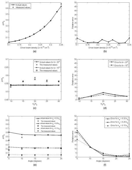
For various driver beam densities, the comparison between the actual and the measured values is shown in

Fig. 6(a) and their relative errors are in Fig. 6(b). The figures show that the relative errors of the measurement do not have any particular trend for the driver beam density less than or equal to0.35n₀. This is where the wakefield FIG. 4. Evolution of the measured density modulation profile resulting from diffraction after the interaction with the wakefield. (a) The profile when it just finishes interacting with the wakefield, (b) when it propagates18μm from the previous picture and (c) after it propagates36μm from the first picture. The shape of the modulated profile is changing and decreases in amplitude as it propagates further from the interaction point.

amplitude reaches∼0.64n₀. It should be noted that none of these errors exceed 10%.

The next comparison is varying the probe’s wavelength from 260 to 800 nm, while the other parameters remain the same as the baseline parameters. The comparison values and the relative errors are shown in Figs.6(c)and(d). These indicate that the error values do not change significantly as the probe’s frequency increases. Therefore the error is independent of the probe’s wavelength.

Another comparison was also done to check the depend-ency of the crossing angle with the measured values using 800 nm probe. This comparison was made with three different values of driver beam density and was designed to cover the linear and nonlinear regimes of the wakefield. The results of this comparison and the errors are shown in Figs. 6(e) and (f). For n_e¼0.15n₀ and n_e ¼0.25n₀, decreasing the crossing angle increases the relative error. This is because when the angle decreases, the interaction length between the wakefield and the probe pulse becomes longer. If the interaction length is comparable to the diffraction length of the modulated part of the pulse, the frequency modulation’s amplitude of the laser pulse decreases because of diffraction, hence increases the relative error. For all cases in Figs. 6(e) and(f), most of the relative errors are less than 10%, except when the crossing angle θ≤10° because of diffraction. This dif-fraction effect will be discussed in the next subsection.

B. Measurement constraints

A photon acceleration diagnostic with oblique angle has several constraints and limitations that can make the measurement results inaccurate. In the previous paper

[33], several limitations in doing the measurement using photon acceleration with a copropagating probe pulse have been discussed. These include maximum propagation distance to avoid photon trapping and maximum intensity of the probe pulse to avoid stimulated Raman scattering. More details can be found in Ref.[33].

In this oblique crossing angle setting, there are more additional constraints. Some of those are apparent in the results provided in the previous subsection. In this sub-section, these new constraints are discussed in greater detail to provide a realistic guide to realize this measurement technique in the laboratory.

1. Diffraction

Consider the electric field of the probe as a function of position, U₀ðr; tÞ ¼ jU₀ðr; tÞjeik·r−iω0t_{. As it crosses the}

wakefield, the probe will experience a phase and frequency modulation. Thus, the modulated electric field profile can now be written as Uðr; tÞ ¼U₀ðr; tÞeiΔϕðr;tÞ, where

Δϕðr; tÞ is the phase modulation resulting from laser-wakefield interaction. If the modulation is small enough, it can be approximated as

Uðr; tÞ≈U₀ðr; tÞ þiU₀ðr; tÞΔϕðr; tÞ: ð14Þ

From the equation above, the modulated part of the probe can be regarded as a new wave propagating in the same direction with approximately same frequency, but with amplitude profile ofjU₀ðr; tÞjjΔϕðr; tÞj.

In the photon acceleration case, when a very wide probe crosses a small wakefield, the probe pulse will have a modulated part with a size approximately the same as that of the wakefield. Because the modulated part has the smaller size, it will diffract faster than the unperturbed part of the probe. This diffraction effect reduces the phase and frequency modulation of the pulse if the interaction length is larger than its diffraction length. In order to minimize the diffraction effect, the crossing angle, θ, should be large enough to keep the interaction length short, or

sinθ≳ λffiffiffi0 π p

r_p ð15Þ

whereλ₀is the probe’s wavelength andrpis the wakefield’s radius.

In the simulated cases, the crossing angle should be θ≳8°. This explains why the relative errors start increasing whenθ¼10° and increase significantly when the crossing angle is set to be 5° for any simulated driver densities as shown in Fig. 6(f).

2. Error dependence on angle

It is interesting to see how the measurement error is related to the angle of incidence. As seen later in this subsection, the error analysis on the angle can set the upper limit of the crossing angle.

In order to simplify the analysis, it is assumed that the wakefield has a perfect sinusoidal in the longitudinal position and a Gaussian profile in the transverse position. Although this is not the case for nonlinear wakefield and some other cases (e.g., non-Gaussian transverse profile of the driver), it is still useful to quantify the error. For this simplified case, the frequency shift of the laser pulse has a similar profile and can be written as

Δω ω0 ¼

Δω ω0

max

sinðω_pζ₀=cÞe−y2=r2p ð₁₆Þ

wherer_prepresents the radius of the wakefield at which the value drops to1=eof the axial value. Other variables are as introduced before. Applying the inverse transformation in Eq.(9), the wakefield density is obtained as

Δn n₀ ¼

Δn n₀

max

sinðωpζ=cÞe−r2=r2p ð17Þ

Δn n₀

max

¼− 2ffiffiffi

π

p ω20cvgsinθ

ω3_puprp e 1 4ω2pa2r2p=c2

Δω ω0

max

: ð18Þ

Notice that the oblique crossing angle raises an exponential effect inðΔn=n₀Þ_maxfor large absolute value ofa. Defining fm≡ðΔn=n0Þmax makes the equation simpler.

If there is an error in quantifying the angle, the contribution of this error from Eq. (18)is

δf_m fm ¼

_ω2 pr2p 2c2

cosθ−u_vp

g

sinθ up

vgcosθ−1

sinθ θþ θ tanθ

δθ

θ: ð19Þ

In most cases of plasma wakefield accelerators, both the probe and the driver travel with speed near the speed of light, so it can be assumed thatu_p=v_g≈1. Thus, Eq. (19)

can be written in a simpler form,

δfm f_m ≈

θ tanθþ

ω2

pr2p 2c2

1−cosθ sinθ

₂

θ

δθ

θ : ð20Þ

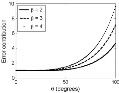
Figure 7 shows how the error contribution from the angle [the term inside the right angle brackets in Eq.(20)] grows as the crossing angle grows for various values of β≡ω2_pr2_p=2c2_{. The graph shows that the error contribution}

grows faster as the crossing angle increases.

From the graph, one can choose the maximum angle that could give reasonable error contribution from the angle. One possible choice of maximum angle is when the error contribution from the angle reaches 2. Other values can be chosen with trade-off between error and the maximum angle. For the simulated cases in this paper, the error from quantifying the angle is doubled whenθ≈60°.

V. CONCLUSIONS

The first quantitative theoretical and simulation studies of photon acceleration diagnostics with oblique crossing

angle on plasma wakefield have been presented. A small intensity probe pulse crosses the wakefield at certain positions with a defined angle of incidence. By choosing the interaction point between the probe and the wakefield, it has been shown here that one can obtain an image of the plasma wakefield density modulation profile at that point. Therefore, it is possible to detect the evolution of plasma wakefield along the propagation distance.

Results from our simulated measurements show that the density modulation measured from the frequency modu-lation profiles of the probe pulse agrees with the actual electron density modulation profiles to within 10% relative error. The constraints that set the lower and upper limit of the crossing angle to minimize errors to obtain electron density modulation profiles are also discussed in this paper. These are the diffraction effect and error dependency analysis on the crossing angle. By considering the con-straints, one can determine the optimal parameters in both laser and beam-driven wakefield accelerators to extract the density modulation profile as a function of position along the plasma column.

ACKNOWLEDGMENTS

The authors would like to acknowledge the support from the plasma physics HEC Consortium EPSRC Grant No. EP/L000237/1, as well as the Central Laser Facility and the Scientific Computing Department at the Rutherford Appleton Laboratory for the use of SCARF-LEXICON computer cluster. We would also like to thank ARCHER UK National Supercomputing Service for the use of the computing service. We also wish to thank the UCLA/IST OSIRIS consortium for the use of OSIRIS and also to the Science and Technology Facilities Council for its support to AWAKE-UK (Grants No. ST/K002244/1 and No. ST/ M007375/1). One of the authors (M. F. Kasim) would like to thank Indonesian Endowment Fund for Education for its support. M. C. L. thanks the Royal Society Newton International Fellowship for support. J. S. and N. R. acknowledge the support from Engineering and Physical Sciences Research Council. M. W. acknowledges the sup-port of DESY, Hamburg, and the Alexander von Humboldt Foundation. The work is part of EuCARD-2, partly funded by the European Commission, GA 312453. The authors gratefully acknowledge the support of all of the staff of STFC’s Central Laser Facility in the execution of this work.

APPENDIX A:

In this part, it will be proven that the y-integral on Eq.(12) is constant, i.e.,

I¼

Z _s

y¼ry

cosðkapffiffiffiffiffiffiffiffiffiffiffiffiffiffis2−y2Þcoshðkapffiffiffiffiffiffiffiffiffiffiffiffiffiffiy2−r2Þ ffiffiffiffiffiffiffiffiffiffiffiffiffiffi

s2_−y2

p ffiffiffiffiffiffiffiffiffiffiffiffiffiffi y2_−r2

p dy¼π

2: FIG. 7. Relative error contribution from the angle to the

wakefield density measurement for various values of β≡ ω2

Substituting x2≡y2−r2 and thus xdx¼ydy into the equation above gives

I¼

Z ffiffiffiffiffiffiffiffiffip_s2_−r2

x¼0

cos½kapffiffiffiffiffiffiffiffiffiffiffiffiffiffiffiffiffiffiffiffiffiffiffiffiffiffiffiðs2−r2Þ−x2coshðkaxÞ ffiffiffiffiffiffiffiffiffiffiffiffiffiffiffiffiffiffiffiffiffiffiffiffiffiffiffi

ðs2_−r2_Þ−x2

p dx:

Now substitutex¼pffiffiffiffiffiffiffiffiffiffiffiffiffiffis2−r2sinθto the equation above so it can be simplified into

I¼

Z _π=2

0 cosðbcosθÞcoshðbsinθÞdθ;

whereb≡kapffiffiffiffiffiffiffiffiffiffiffiffiffiffis2−r2. Using the representation of cosine and hyperbolic cosine in exponential form, the integral can be further simplified into

I¼1

2 Z _π=2

−π=2cosðbe

iθ_Þdθ:

Taking the derivative of I with respect tobyields

∂I ∂b¼−

1 2

Z _π=2

−π=2e

iθ_sinðbeiθ_Þdθ

¼ 1

2ibcosðbeiθÞj

π=2

−π=2¼0:

Zero derivative ofImeans that value ofIdoes not depend onb. Thus, the integral can be evaluated at limitb→0to get the value of the integral,

I¼lim b→0

1 2

Z _π=2

−π=2cosðbe

iθ_Þdθ¼π

2

as used in Eq.(13).

APPENDIX B:

The inverse of modified Abel transformation in Eq.(9)

contains singularity when y¼r. The modified 3-points Abel inversion can be employed to overcome this problem in the implementation.

First, the integral term in Eq. (9) is split into several integrals with spacingΔr,

fðr_jÞ ¼−1

π X i≥j Z _y if yi0

F0_ðyÞcosh

ka ffiffiffiffiffiffiffiffiffiffiffiffiffiffiy2_−r2

j

q

ffiffiffiffiffiffiffiffiffiffiffiffiffiffi y2_−r2

j

q dy;

where rj¼jΔr, yif ¼iΔrþΔr=2, yi0¼iΔrþgijΔr, and

gij¼ 0₋₁₌₂ if_otherwise:i¼j

Note that the second argument, k, and the tilde hat from ~

fðr; kÞandF~ðy; kÞin Eq.(9) are dropped for the sake of simplicity. The term∂F=~ ∂yis denoted byF0.

Substitutingr_j¼jΔrandy¼iΔrþδΔrto the integral gives

fðrjÞ

¼−1

π

X

i≥j Z ₁₌₂

gij

F0_{ðiΔrþδΔrÞcoshðkaΔr}p_ðffiffiffiffiffiffiffiffiffiffiffiffiffiffiffiffiffiffiffiffiffi_iþδÞ2_−j2_Þ

ffiffiffiffiffiffiffiffiffiffiffiffiffiffiffiffiffiffiffiffiffiffiffi

ðiþδÞ2_−j2

p dδ:

The termF0ðiΔrþδΔrÞand the hyperbolic cosine term can be expanded using Taylor series aroundiΔrto the first order. The expansions are

F0_{ðiΔrþδΔrÞ≈F}0_{ðiΔrÞ þF}00_{ðiΔrÞδΔr}

and

cosh

kaΔrqffiffiffiffiffiffiffiffiffiffiffiffiffiffiffiffiffiffiffiffiffiffiffiffiffiðiþδÞ2_−j2_¼C

ijþSijδ;

where F00 is the second derivative of the function F relative to y, Cij¼coshðkaΔr

ffiffiffiffiffiffiffiffiffiffiffiffiffi i2_−j2

p

Þ, and Sij¼ sinhðkaΔrpffiffiffiffiffiffiffiffiffiffiffiffiffii2−j2ÞkaiΔr=pffiffiffiffiffiffiffiffiffiffiffiffiffii2−j2.

Substituting these two expanded terms in the integral and keeping only the first order terms of δ leaves us an analytically integrable expression. Evaluating the integral analytically leaves us the equation below,

fðrjÞ ¼−1

π

X

i≥j

fF0

iCijBðij0Þþ ½F00iΔrCijþF0iSijBðij1Þg;

whereFi is a shorthand forFðiΔrÞ and

Bð_ij0Þ¼

8 > > > > > > < > > > > > > :

0 ;i¼j¼0 or i < j

ln

2iþ1þpðffiffiffiffiffiffiffiffiffiffiffiffiffiffiffiffiffiffi2iþ1Þ2_−4j2 2i

;i¼j≠0

ln

2iþ1þpðffiffiffiffiffiffiffiffiffiffiffiffiffiffiffiffiffiffi2iþ1Þ2_−4j2 2i−1þpffiffiffiffiffiffiffiffiffiffiffiffiffiffiffiffiffiffið2i−1Þ2_−4j2

;i > j

Bð_ij1Þ¼

8 > > < > > :

0 ;i¼j¼0 or i < j Dþ

ij−iBðij0Þ ;i¼j≠0 Dþ

ij−D−ij−iBðij0Þ ;i > j;

withD_ij≡pffiffiffiffiffiffiffiffiffiffiffiffiffiffiffiffiffiffiffiffiffiffiffiffiffiffiffiffiffiffiði1=2Þ2−j2.

In quadratic interpolation, the first and second derivative of the functionF can be expressed as

F0

i¼ ðFiþ1−Fi−1Þ=2Δr

F00

i ¼ ðFiþ1þFi−1−2FiÞ=Δr2:

fðrjÞ ¼− 1

πΔr X

i≥j

Fi½−2CijBðij1Þ

þF_i−1

−₂1CijBðij0ÞþCijBijð1Þ−1₂SijBðij1Þ

þF_iþ1

1 2CijB

ð0Þ

ij þCijBðij1Þþ1₂SijBðij1Þ

:

The 3-points Abel inversion method is similar with the technique described in Ref.[39], except that the hyperbolic cosine term is also expanded in this method.

Another problem that may arise in the implementation is that the hyperbolic cosine term can amplify the high frequency noise. This problem can be solved simply by choosing a cutoff value,k_c and set k¼0 whenk≥k_c.

[1] T. Tajima and J. M. Dawson, Phys. Rev. Lett. 43, 267 (1979).

[2] A. Modena, Z. Najmudin, A. E. Dangor, C. E. Clayton, K. A. Marsh, C. Joshi, V. Malka, C. B. Darrow, C. Danson, D. Neelyet al.,Nature (London)377, 606 (1995). [3] C. Joshi, W. B. Mori, T. Katsouleas, J. M. Dawson, J. M.

Kindel, and D. W. Forslund, Nature (London) 311, 525 (1984).

[4] S. P. D. Mangles, C. D. Murphy, Z. Najmudin, A. G. R. Thomas, J. L. Collier, A. E. Dangor, E. J. Divall, P. S. Foster, J. G. Gallacher, C. J. Hooker et al., Nature (London)431, 535 (2004).

[5] C. G. R. Geddes, Cs. Toth, J. van Tilborg, E. Esarey, C. B. Schroeder, D. Bruhwiler, C. Nieter, J. Cary, and W. P. Leemans,Nature (London)431, 538 (2004).

[6] J. Faure, Y. Glinec, A. Pukhov, S. Kiselev, S. Gordienko, E. Lefebvre, J.-P. Rousseau, F. Burgy, and V. Malka,Nature (London)431, 541 (2004).

[7] W. P. Leemans, B. Nagler, A. J. Gonsalves, Cs. Tóth, K. Nakamura, C. G. R. Geddes, E. Esarey, C. B. Schroeder, and S. M. Hooker,Nat. Phys.2, 696 (2006).

[8] V. Malka, S. Fritzler, E. Lefebvre, M.-M. Aleonard, F. Burgy, J.-P. Chambaret, J.-F. Chemin, K. Krushelnick, G. Malka, S. P. D. Mangleset al.,Science298, 1596 (2002). [9] F. Amiranoff, S. Baton, D. Bernard, B. Cros, D. Descamps, F. Dorchies, F. Jacquet, V. Malka, J. R. Marquès, G. Matthieussentet al.,Phys. Rev. Lett.81, 995 (1998). [10] Y. Kitagawa, T. Matsumoto, T. Minamihata, K. Sawai, K.

Matsuo, K. Mima, K. Nishihara, H. Azechi, K. A. Tanaka, H. Takabeet al.,Phys. Rev. Lett.68, 48 (1992). [11] C. E. Clayton, K. A. Marsh, A. Dyson, M. Everett, A. Lal,

W. P. Leemans, R. Williams, and C. Joshi,Phys. Rev. Lett.

70, 37 (1993).

[12] F. Amiranoff, D. Bernard, B. Cros, F. Jacquet, G. Matthieussent, P. Miné, P. Mora, J. Morillo, F. Moulin, A. E. Speckaet al.,Phys. Rev. Lett.74, 5220 (1995). [13] J. B. Rosenzweig, D. B. Cline, B. Cole, H. Figueroa, W.

Gai, R. Konecny, J. Norem, P. Schoessow, and J. Simpson,

Phys. Rev. Lett.61, 98 (1988).

[14] I. Blumenfeld, C. E. Clayton, F.-J. Decker, M. J. Hogan, C. Huang, R. Ischebeck, R. Iverson, C. Joshi, T. Katsouleas, N. Kirbyet al.,Nature (London)445, 741 (2007). [15] P. Muggli, B. E. Blue, C. E. Clayton, S. Deng, F.-J. Decker,

M. J. Hogan, C. Huang, R. Iverson, C. Joshi, T. C. Katsouleaset al.,Phys. Rev. Lett.93, 014802 (2004). [16] A. Caldwell, K. Lotov, A. Pukhov, and F. Simon, Nat.

Phys.5, 363 (2009).

[17] N. Kumar, A. Pukhov, and K. Lotov,Phys. Rev. Lett.104, 255003 (2010).

[18] M. Litos, E. Adli, W. An, C. I. Clarke, C. E. Clayton, S. Corde, J. P. Delahaye, R. J. England, A. S. Fisher, J. Fredericoet al.,Nature (London)515, 92 (2014). [19] E. Esarey, C. B. Schroeder, and W. P. Leemans,Rev. Mod.

Phys.81, 1229 (2009).

[20] D. Gordon, K. C. Tzeng, C. E. Clayton, A. E. Dangor, V. Malka, K. A. Marsh, A. Modena, W. B. Mori, P. Muggli, Z. Najmudinet al.,Phys. Rev. Lett.80, 2133 (1998). [21] N. H. Matlis, S. Reed, S. S. Bulanov, V. Chvykov, G.

Kalintchenko, T. Matsuoka, P. Rousseau, V. Yanovsky, A. Maximchuk, S. Kalmykovet al.,Nat. Phys.2, 749 (2006). [22] K. Y. Kim, I. Alexeev, and H. M. Milchberg,Appl. Phys.

Lett.81, 4124 (2002).

[23] Z. Li, R. Zgadzaj, X. Wang, Y.-Y. Chang, and M. C. Downer, Nat. Commun.5, 3085 (2014).

[24] A. Maksimchuk, S. Reed, S. S. Bulanov, V. Chvykov, G. Kalintchenko, T. Matsuoka, C. McGuffey, G. Mourou, N. Naumova, J. Neeset al.,Phys. Plasmas15, 056703 (2008). [25] Z. Li, H.-E. Tsai, X. Zhang, C.-H. Pai, Y.-Y. Chang, R. Zgadzaj, X. Wang, V. Khudik, G. Shvets, and M. C. Downer, Phys. Rev. Lett.113, 085001 (2014).

[26] A. Buck, M. Nicolai, K. Schmid, C. M. S. Sears, A. Sävert, J. M. Mikhailova, F. Krausz, M. C. Kaluza, and L. Veisz,

Nat. Phys.7, 543 (2011).

[27] A. Sävert, S. P. D. Mangles, M. Schnell, J. M. Cole, M. Nicolai, M. Reuter, M. B. Schwab, M. Möller, K. Poder, O. Jäckelet al.,arXiv:1402.3052.

[28] S. C. Wilks, J. M. Dawson, W. B. Mori, T. Katsouleas, and M. E. Jones,Phys. Rev. Lett.62, 2600 (1989).

[29] J. M. Dias, L. Oliveira e Silva, and J. T. Mendonça,Phys. Rev. ST Accel. Beams1, 031301 (1998).

[30] C. D. Murphy, R. Trines, J. Vieira, A. J. W. Reitsma, R. Bingham, J. L. Collier, E. J. Divall, P. S. Foster, C. J. Hooker, A. J. Langley et al., Phys. Plasmas 13, 033108 (2006).

[31] R. M. G. M. Trines, C. D. Murphy, K. L. Lancaster, O. Chekhlov, P. A. Norreys, R. Bingham, J. T. Mendonça, L. O. Silva, S. P. D. Mangles, C. Kamperidiset al.,Plasma Phys. Controlled Fusion51, 024008 (2009).

[32] J. T. Mendonça, Theory of Photon Acceleration (CRC Press, Bristol, 2001).

[33] M. F. Kasim, N. Ratan, L. Ceurvorst, J. Sadler, P. N. Burrows, R. Trines, J. Holloway, M. Wing, R. Bingham, and P. Norreys, Phys. Rev. ST Accel. Beams18, 032801 (2015).

[34] C. J. Dasch,Appl. Opt.31, 1146 (1992).

[37] N. H. Abel,Résolution d’un problème de mecanique, 1826, Oeuvres Complètes, Vol. 1 (Christiania, Oslo, 1881), p. 97. [38] N. H. Abel, Journal für die reine und angewandte

Mathematik,1, 153 (1826).

[39] A. M. Cormack,J. Appl. Phys.34, 2722 (1963). [40] R. A. Fonseca, L. O. Silva, F. S. Tsung, V. K. Decyk, W.

Lu, C. Ren, W. B. Mori, S. Deng, S. Lee, T. Katsouleas et al., Lecture Notes in Computer Science Vol. 2329, III-342(Springer, Heidelberg, 2002).

[41] R. G. Hemker,arXiv:1503.00276.

[42] C. K. Birdsall and A. B. Langdon, Plasma Physics via Computer Simulation(CRC Press, Bristol, 2004). [43] C. W. Siders, S. P. Le Blanc, A. Babine, A. Stepanov, A.

Sergeev, T. Tajima, and M. C. Downer,IEEE Trans. Plasma Sci.24, 301 (1996).

[44] S. P. Le Blanc, E. W. Gaul, N. H. Matlis, A. Rundquist, and M. C. Downer,Opt. Lett.25, 764 (2000).

[45] C. Iaconis and I. A. Walmsley,Opt. Lett.23, 792 (1998).

[46] J. W. Goodman, Introduction to Fourier Optics