A Savings Plan with Targeted Contributions

City, University of London Institutional Repository

Citation: Owadally, I., Haberman, S. & Gomez, D. (2011). A Savings Plan with Targeted

This is the accepted version of the paper.

This version of the publication may differ from the final published

version.

Permanent repository link: http://openaccess.city.ac.uk/14280/

Link to published version: http://dx.doi.org/10.1111/j.1539-6975.2012.01485.x

Copyright and reuse: City Research Online aims to make research

outputs of City, University of London available to a wider audience.

Copyright and Moral Rights remain with the author(s) and/or copyright

holders. URLs from City Research Online may be freely distributed and

linked to.

City Research Online: http://openaccess.city.ac.uk/ publications@city.ac.uk

A Savings Plan with Targeted Contributions

Iqbal Owadally

, Steven Haberman

, Denise Gomez-Hernandez

30 November 2011

The final version of this paper is published in the Journal of Risk and Insurance.

Abstract

We consider a simple savings problem where contributions are made to a fund and invested

to meet a future liability. The conventional approach is to estimate future investment

return and calculate a fixed contribution to be paid regularly by the saver. We propose

a flexible plan where contributions are systematically adjusted and targeted. We show

by means of stochastic simulations that this plan has a reduced risk of a shortfall and

is relatively insensitive to errors in the planner’s estimate of future returns. Sensitivity

analyses in terms of parameter values, stochastic return models and investment horizons

are also performed.

Keywords: Savings plan, contributions, pension plans

∗_{Corresponding author: Faculty of Actuarial Science and Insurance, Cass Business School, City}

Uni-versity, 106 Bunhill Row, London EC1Y 8TZ, UK. Phone: +44 (0)20 7040 8478. Fax: +44 (0)20 7040

8572. E-mail: M.I.Owadally@city.ac.uk.

†_{Cass Business School, City University, London.}

‡_{Universidad Aut´onoma de Quer´etaro, Quer´etaro, Mexico.}

Introduction

We consider a simple savings problem where an individual puts aside funds in order to

meet a certain liability at a given date in the future. The individual may contribute to a

medium-term investment and savings vehicle, for example, to meet school or college fees for

his children in 5 years’ time. Another example is where the individual wishes to purchase

property. He may save for, say 5 years, and then withdraw some or all of his investment

and use it as a deposit or down-payment as part of a home loan. A longer-term example

is a retirement or pension fund, where the individual saves out of labor income to provide

a lump sum at retirement. This may then be used to buy an annuity.

In most problems of this kind, a financial planner or adviser will assist the individual

to determine how much he should save and invest every month (say), depending on his

household finances. Two related decisions must be made: how much the monthly

contri-bution will be, and where the savings will be invested. In this paper, we do not consider

the second decision, i.e. asset allocation, although we discuss this briefly later. We assume

instead that the individual saves in a variable-rate bank account or in a low-risk mutual

fund.

A very risk-averse investor could save in a term-deposit bank account or in a

zero-coupon bond, yielding a fixed interest rate. However, it could be that a medium-term

fixed-income investment like this is unavailable or pays unattractive rates. A less

risk-averse investor, such as a young worker aspiring to home-ownership, may instead wish to

invest in a stock market fund to try and achieve the largest possible future down-payment

as part of a home loan. If his stock market investment performs poorly after 5 years, this

may mean that a smaller home loan, or a more expensive loan with a higher debt-to-equity

ratio, will be available to him. On the other hand, a worker who is close to retirement

retirement.

In standard economic theory, this savings problem can be cast as a

consumption-investment problem, with consumption (or saving) and asset allocation as decision

vari-ables, and with a utility or loss function as an objective criterion that is optimized

dynami-cally. Even though idealized assumptions may be made, this approach can lead to decision

rules that are simple to implement and that can be used to benchmark performance. In

practice, however, financial planners do not employ stochastic dynamic optimization to

provide retail advice to individual savers. They will suggest instead that the individual

sets aside a given amount every month, or possibly a fixed percentage of income, and

will also offer suggestions regarding asset allocation. Dynamic optimization is not used

regularly by financial planners at a retail level because of the complications caused by

real-world features such as taxes, transaction costs and investment charges, because of

imperfect knowledge about asset return distributions, and because it is difficult to capture

individuals’ varying financial circumstances and requirements.

One example is in the deterministic lifestyling strategies commonly employed in

target-date funds and in pension planning (Shiller, 2005; Blake, Cairns and Dowd, 2001). Advisers

typically suggest a fixed monthly contribution based on a range of assumed investment

rates of return (Employee Benefits Security Administration, 2006). Another example is

work-related savings vehicles, such as an employer-sponsored pension plan, where a fixed

proportion of salary is determined (McGill et al., 2004). The new Florida public sector

pension plan described by Lachance, Mitchell and Smetters (2003) requires that individuals

save a uniform 9% of pay. The Actuarial Foundation and WISER (2004) suggest a rule of

thumb of saving 15% of pay towards retirement.

Our approach in this paper is to try to improve upon the conventional fixed-contribution

approach. We suggest a flexible targeted-contribution savings plan which has variable

whether this new plan performs robustly, in terms of meeting an investment target at a

given horizon, under a wide range of investment conditions. We show, by means of

sim-ulations, that this plan is less risky than the conventional fixed-contribution plan. Our

proposed savings plan is based on a method used in industrial process control (for

ex-ample, Box and Luce˜no, 1995). The method has also been proposed in the econophysics

literature (Gandolfi, Sabatini and Rossolini, 2007) and is applied in the pensions literature

to defined benefit pension funding with deterministic economic scenarios (Owadally, 2003).

The innovation in this paper is to apply this method to a savings problem with a simple

stochastic investment environment.

In the next section, we describe the targeted-contribution plan. We then run

stochas-tic simulations with serially independent normally distributed log-returns to compare the

performance of this plan over a 5-year saving period with a conventional plan. We measure

the risk that end-of-period wealth falls short of the target liability using both the

stan-dard deviation and 95th percentile. The sensitivity of our proposed plan to the financial

planner’s assumptions is verified by repeating the simulations with different parameter

values. We also run simulations with constraints imposed on the flexible contributions,

with non-Gaussian investment returns incorporating jumps, and with serially correlated

returns. Finally, we consider an application in pension funding with a long investment

horizon and with a bootstrap stochastic asset model using 59 years of investment data on

equities and bonds.

Fixed- and Targeted-Contribution Plans

We set up and compare two savings plans here. The first plan that we consider is a

conventional savings plan where a level contribution is paid regularly. We refer to this as a

be reached at a time horizon T (in months). A financial planner makes an estimate of the

future monthly rate of return. This estimate is typically based on the planner’s statistical or

stochastic model of asset returns, and on an informed view of macro-economic conditions or

market performance. We denote this estimate or return assumption byiA. The individual

contributes a constant amount C at the beginning of every month, which is calculated by

amortizingF at rateiAoverT months, i.e. the stream of monthly contributions in advance

accumulate at rate iA toF.

F = C(1 +iA)i

−1

A ((1 +iA)T −1) (1)

If the fund is invested in risky securities, then the actual rate of return on the fund,

denoted byitin month (t−1,t), is random. The corresponding log-return isδt= ln(1+it).

Let the value of the fund at time t be Ft, with F0 = 0. Then,

Ft+1 = (1 +it+1) (Ft+C) (2)

The value FT of the fund at time T is random and, except by chance, will differ from the

desired fund target F. A terminal or final deficit will therefore emerge at timeT:

DT = F −FT. (3)

The risk for the individual saver is that there is a large deficit at time T. (A surplus is

just a negative deficit here.)

The second plan that we consider is a targeted-contribution plan. This is based on the

pension funding method discussed by Owadally (2003) and adapted from industrial process

control (Box and Luce˜no, 1995). Although we do not consider the asset allocation problem

in this paper, it is worth noting that Gandolfi, Sabatini and Rossolini (2007) propose a

similar method for tactical asset allocation in an investment portfolio.

contribution payment Ct for month (t,t+ 1) as follows:

Ct = C + λ1Dt + λ2

∞ X

j=0

Dt−j (4)

whereλ1 andλ2 are variables to be specified. subject to the constraintsλ1 >0 andλ2 >0.

We assume that Dt = 0 for t < 0. Here Dt represents the notional deficit at time t in

the fund, relative to what the value of the fund would be if the individual followed the

fixed-contribution plan and if the fund earned the anticipated return iA every month.

Dt = C(1 +iA)i

−1

A ((1 +iA)t−1) − Ft (5)

Equation (4) therefore requires that, at time t, an overpayment at a rate ofλ1 is made

based on the notional deficit Dt. If actual returns on the fund are persistently lower than

the anticipated return iA, then deficits will recur systematically. Therefore, equation (4)

also imposes a further overpayment, at a rate ofλ2, based on the cumulative sum of deficits

up to timet. If there is no persisting deficit, i.e. positive and negative deficits cancel each

other out on average, then the additional overpayment represented by the third term on

the right hand side of equation (4) is on average zero.

We do not directly address the optimal choice of parametersλ1 andλ2 here. Instead we

assume a set of practical parameter values and investigate the targeted-contribution plan

under various conditions such as the presence of parameter estimation errors, persistence

and jumps in investment returns, investor cash flow constraints, and long-term retirement

planning objectives. Our aim is to establish robustness of the targeted-contribution

ap-proach, and we leave formal optimization to future work.

Practical values for λ1 and λ2 in equation (4) are likely to be small because a saver

may be unable or unwilling to make additional contributions, and tax advantages may also

mean that he is unwilling to reduce his contributions. In the following, our base parameter

values are λ1 = 0.2 = 1

(ignoring interest), and λ2 = 0.01 as a charge or tax of 1% per month thereafter on the

deficit in any month. These parameter values are comparable to values employed by Box

and Luce˜no (1995) and Owadally (2003) in other contexts. In a later section, we consider

other values for λ1 andλ2 and we also discuss parameter choice by reference to an ARMA

time series process.

Results of Stochastic Simulations

Stochastic simulations are performed to compare the terminal deficits under the two plans

described in the preceding section. An investment horizon ofT = 60 months and a target

fund of F = 100 are assumed, along with values λ1 = 0.2 and λ2 = 0.01 in the

targeted-contribution plan in equation (4). 10,000 simulations were carried out throughout, with

frequent checks for convergence using 5,000 and 20,000 simulations, and with a fixed seed

for the random number generator to minimize sampling error when comparing results.

The monthly logarithmic returnδt = ln(1 +it) on the fund is simulated as an

indepen-dent and iindepen-dentically distributed (iid) sequence of normally distributed random numbers

with mean 0.3792% and standard deviation 2%. The mean arithmetic return is thus 0.4%

per month. These are representative values for a relatively conservative investment fund.1

A financial planner has to estimate future investment return and make an assumptioniA

as to the return on the fund. Since he does not have perfect foresight, he may over- or

1_{The values are chosen for illustrative purposes. (Simulations using 59 years of asset return data are}

performed in a subsequent section.) For comparison, Friesen and Sapp (2007) use the CRSP

Survivor-Bias-Free US Mutual Fund database with returns over the 1991-2004 period and simulate stock market

mutual funds with a geometric monthly return that is i.i.d. normally distributed with a mean of 0.75%

and standard deviation of 5%. They also provide geometric monthly return statistics for bond funds

(mean=0.43%, s.d.=0.30%) and money market funds (mean=0.24%, s.d.=0.14%). The simulated fund

here can be seen as invested in a range of asset classes and to be less risky than a stock market fund but

under-estimate future average investment return. For example, if iA = 0.7%, the planner

overestimates the mean return by 0.3% per month. Henceforth, we define the estimation

error as the excess of iA over the average return on the fund. When iA = 0.7%, the

planner’s estimation error is therefore 0.3% per month.

Histograms of Terminal Deficit

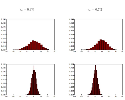
Figure 1 shows the distributions of the terminal deficit under the two plans, for iA= 0.4%

and 0.7%. Since the accumulated fund has a right-skewed distribution, the distribution of

the deficit is left-skewed. We make two observations.

Observation 1 _{The fixed-contribution plan is riskier than the targeted-contribution plan}

(where we measure risk in terms of the fund falling short of the target at the end-date).

The terminal deficit is more dispersed under the fixed-contribution plan (top panels

in Figure 1) than under the targeted-contribution plan (bottom panels in Figure 1). The

fixed-contribution plan is riskier than the targeted-contribution plan in that end-wealth is

more volatile and has a heavier-tailed distribution in the former case than in the latter

case.

Observation 2 _{Risk in the fixed-contribution plan is sensitive to the error in the financial}

planner’s estimate of future investment return, whereas risk in the targeted-contribution

plan is relatively insensitive to this. (Again, we measure risk in terms of the shortfall or

deficit from the target at the end.)

When the return assumption is 0.7%, rather than 0.4%, the adviser’s return assumption

overstates the mean return on the fund and we anticipate that the plans will, on average,

fall short of the target. The distribution of the terminal deficit does indeed shift to the

iA= 0.4% iA= 0.7%

Figure 1: Histograms for the terminal deficit under fixed-contribution plan (top panels)

and targeted-contribution plan (bottom panels). F = 100, δt ∼ iid N(0.003792, 0.022),

λ1 = 0.2 andλ2 = 0.01. Statistics appear in Table 1.

plan. However, it remains centered around zero in the targeted-contribution plan. If the

planner’s return assumption turns out to be over-optimistic, the risk of a shortfall is greater

in the fixed-contribution plan than in the targeted-contribution plan.

Percentiles and Moments of Terminal Deficit

Table 1 shows how various statistics concerning the terminal deficit change as the

Error Mean deficit St. deviation 95th percentile Mean square

iniA of deficit of deficit deficit

FC TC FC TC FC TC FC TC

-0.3% -9.841 -0.497 10.385 3.223 6.219 4.697 204.701 10.636

-0.2% -6.499 -0.336 10.068 3.214 9.073 4.843 143.600 10.442

-0.1% -3.230 -0.171 9.760 3.205 11.863 4.998 105.691 10.299

0 -0.036 -0.003 9.458 3.195 14.591 5.155 89.453 10.210

0.1% 3.086 0.169 9.163 3.186 17.256 5.315 93.478 10.178

0.2% 6.135 0.344 8.875 3.176 19.859 5.472 116.394 10.207

0.3% 9.112 0.523 8.593 3.167 22.401 5.641 156.866 10.301

Table 1: Mean, standard deviation, mean square and 95th percentile of terminal deficits

under fixed-contribution plan (FC) and targeted-contribution plan (TC). The error iniA

is the excess of iA over the average return. F = 100, δt∼iid N(0.003792, 0.022), λ1 = 0.2

and λ2 = 0.01.

First, note that the 95th percentile and standard deviation of the terminal deficit are

smaller in the targeted-contribution plan than in the fixed-contribution plan for all values

of errors in iA in Table 1. The histograms in Figure 1 illustrate this visually for errors of

0 and 0.3%. This confirms Observation 1 above.

Secondly, note that the more iA overestimates the average return (i.e. the greater the

error in iA), the greater the terminal deficit in the fixed-contribution plan: both the mean

deficit and the 95th percentile of the deficit increase. The targeted-contribution plan,

however, is much less sensitive to the error in iA: the mean, standard deviation and 95th

percentile of the deficit change, but not as much as in the fixed-contribution case. This

confirms Observation 2 above. The mean square deficit column in Table 1 gives the second

the targeted-contribution plan is fairly constant regardless of the size of the error.

Finally, we also computed skewness and kurtosis. The coefficients of skewness are

−0.319 and −0.107 (to 3 d.p.) for the fixed-contribution and targeted-contribution plans respectively, for all estimation errors in Table 1. The top panels in Figure 1 exhibit a more

pronounced left skew than the bottom panels. The respective coefficients of kurtosis are

3.305 and 3.002 (to 3 d.p.) for all estimation errors in Table 1.

Discussion of Results and Sensitivity Analysis

Observations 1 and 2

Observation 1, i.e. that the targeted-contribution plan is less risky than the

fixed-contri-bution plan, in terms of meeting the target at the investment horizon, is not surprising.

The targeted-contribution plan is flexible and contributions can be varied to make up any

shortfall gradually. In other words, the flexible contributions pick up part of the investment

risk, thereby reducing the risk to end-wealth.

Observation 2, i.e. that the targeted-contribution plan is relatively insensitive to errors

in the planner’s estimate of investment return, is less intuitively obvious. Whereas the

first observation could arise from any plan that allows flexible contributions, the second

observation requires that the contributions be flexible and be targeted systematically, so

as to counter the effect of the estimation error. The third term on the right hand side of

equation (4) ensures that any notional deficit that accumulates over time is ‘taxed’ at a

rate λ2, thereby adjusting the contribution to restore the savings plan on a path to target.

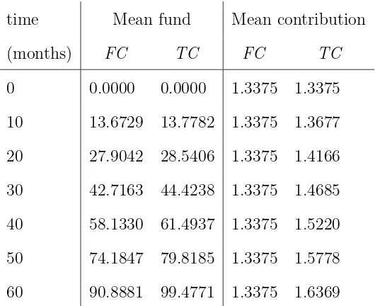
This is illustrated in Table 2 which shows the average path of the two plans over time for

a return assumption of 0.7%. The fund builds up gradually from 0 to about 90 on average

in the fixed-contribution plan, leaving an average terminal shortfall of 10. By contrast,

time Mean fund Mean contribution

(months) FC TC FC TC

0 0.0000 0.0000 1.3375 1.3375

10 13.6729 13.7782 1.3375 1.3677

20 27.9042 28.5406 1.3375 1.4166

30 42.7163 44.4238 1.3375 1.4685

40 58.1330 61.4937 1.3375 1.5220

50 74.1847 79.8185 1.3375 1.5778

60 90.8881 99.4771 1.3375 1.6369

Table 2: Mean values of fund and contribution over time under fixed-contribution plan

(FC) and targeted-contribution plan (TC). F = 100, δt ∼ iid N(0.003792, 0.022), iA =

0.7%, λ1 = 0.2 and λ2 = 0.01.

almost no terminal shortfall on average. Whereas the contribution is constant under the

fixed-contribution plan, the mean contribution in the targeted-contribution plan gradually

increases so that the plan is on average on target after 60 months.

An estimation error in the financial planner’s investment return assumption can arise

in several ways. The planner’s model of asset returns may be wrongly calibrated because

of insufficient or inaccurate data (parameter risk). The model itself may be mis-specified

(model risk). For example, the planner may fit a normal distribution to asset returns

that, in fact, have a heavy-tailed distribution, thereby discounting the effect of market

corrections and underestimating tail risk. An estimation error may also occur because of

a large unexpected shift in the economic environment (such as after a market crash or

following a revision in monetary policy targets by the central bank). Finally, and more

subtly, the financial planner may exhibit behavioral biases, leading to overconfidence in

time Var fund Var contribution

(months) FC TC TC

0 0 0 0

10 0.3581 0.1764 0.0089

20 2.7890 0.8225 0.0443

30 9.7172 2.0260 0.1102

40 23.9019 3.8799 0.2104

50 48.9548 6.5508 0.3520

60 88.3625 10.0954 0.5393

Table 3: Variance of fund and contribution over time under fixed-contribution plan (FC)

and targeted-contribution plan (TC). Contribution under FC has zero variance. F = 100,

δt∼iid N(0.003792, 0.022),iA = 0.4%, λ1 = 0.2 andλ2 = 0.01.

influenced by framing and mental accounting issues (Thaler, 1999). Observation 2 therefore

suggests that the targeted-contribution plan performs fairly robustly regardless of all these

sources of estimation errors in the future investment return.

Terminal Wealth and Interim Consumption

The targeted-contribution savings plan shifts uncertainty from terminal wealth to

inter-mediate contributions. For a short-term savings plan, or one where contribution is a small

proportion of income, the variability in contributions may have a negligible impact on the

saver and on the saver’s consumption during the saving period. On the other hand, for

a long-term savings plan, or one where the contribution is a large proportion of income,

large contribution requirements over a long period could be unaffordable.

estimate iA = 0.4%. First, we calculate the variance of the fund and contribution at

intermediate time steps.2

The results are displayed in Table 3. The contribution variance

over time in the fourth column is significantly smaller than the variance in terminal wealth

(at timet= 60) for either the fixed-contribution plan (88.363) or the targeted-contribution

plan (10.095). Much more of the “total variance” is allocated to end-wealth than to interim

contributions.

Secondly, we recognize that individuals may have cash flow constraints. We repeat

the earlier simulations except that we use a constrained contribution Cet in the

targeted-contribution plan:

e Ct =

              

0 if Ct<0

u C if Ct> u C

Ct otherwise

(6)

where Ct is as in equation (4), C is the planned contribution in the fixed-contribution

savings plan, and u provides an upper constraint relative to C, with u ≥1. The larger u

is, the less budget-constrained the saver is, i.e. the more he is able to afford contributions

that are larger than planned if investment returns are unfavorable.

We anticipate that, the more budget-constrained the saver is, the more increases in

contribution will be limited, and the less effective the targeted-contribution plan will be

in compensating for lower than anticipated investment returns. Table 4 does indeed show

that, the lower u is, the more end-wealth risk increases in the targeted-contribution plan:

the volatility and 95th percentile of terminal deficits in the targeted-contribution plan

increase with decreasingu.

2_{We should ideally consider the variance of fund and contribution relative to labor income, as do Cairns,}

Blake and Dowd (2006) (among others) who consider a power utility function_γ1W_Y((_TT₎)γof terminal wealth

W(T) relative to terminal incomeY(T) at time horizonT. However, in our setting, scaling contribution

Mean deficit St. deviation 95th percentile

of deficit of deficit

FC TC FC TC FC TC

no constraint -0.036 -0.003 9.458 3.195 14.591 5.155

u= 2 -0.036 -0.015 9.458 3.249 14.591 5.185

u= 1.75 -0.036 0.044 9.458 3.310 14.591 5.465

u= 1.5 -0.036 0.270 9.458 3.530 14.591 6.189

u= 1.25 -0.036 1.072 9.458 4.215 14.591 8.560

u= 1.1 -0.036 2.451 9.458 5.153 14.591 11.806

u= 1.05 -0.036 3.313 9.458 5.631 14.591 13.397

Table 4: Mean, standard deviation and 95th percentile of terminal deficits under

fixed-contribution plan (FC) and targeted-contribution plan (TC), for various upper constraint

factor u. FC is independent of u but statistics are shown for comparison. F = 100,

δt∼iid N(0.003792, 0.022),iA = 0.4%, λ1 = 0.2 andλ2 = 0.01.

The upper constraintudoes not affect the fixed-contribution plan, of course, but

statis-tics are shown in Table 4 for the sake of comparison. We observe from Table 4 that

the targeted-contribution plan, even when constrained, performs better than the

fixed-contribution plan in terms of achieving a lower end-wealth risk. It is also of practical

inter-est to note that, even if contributions in the targeted-contribution plan are constrained to be

no more than 110% of the planned contribution under the conventional fixed-contribution

plan (and no less than zero), the standard deviation of the terminal deficit is reduced by

almost half.

Constraining contributions as in equation (6) may be realistic to the extent that

every month. Nevertheless, the analysis in this paper is limited in that risk is measured in

terms of terminal wealth only. We note, as a direction for future research, that one could

consider utility over both end-wealth and the interim consumption stream. Labor income

risk then becomes relevant (Campbell and Viceira, 2002). If labor income is inversely

cor-related with investment return, a hedging effect is induced which may reduce combined

risk in terms of both consumption and end-wealth.

The intermediate consumption pattern also matters in conventional fixed-contribution

plans, in fact. A prudent financial adviser will underestimate future investment return

(that is, he will end up with negative values of the estimation error in Table 1) so as to

minimize the 95th percentile of deficits. However, this can also result in large surpluses, in

the individual making larger contribution payments than he can afford, and in a consequent

loss in utility of consumption during the saving period. Again, we note this here as an

item for further research.

Variables λ1 and λ2

Simulations for a wider range of values of λ1 and λ2 are described in the Appendix.

Our main conclusion is that the targeted-contribution plan is less risky than the

fixed-contribution plan, in terms of volatility and 95th percentile of the deficit, for all but

impractically large values of λ1 and λ2. For example, the targeted-contribution plan is

less risky than the fixed-contribution plan for λ1 ≤ 2 when λ2 = 0.01 (Table 11 in the

Appendix) or λ2 ≤ 3 when λ1 = 0.2 (Table 12 in the Appendix). We also find that

the volatility of contributions increases as λ1 and λ2 increase. This is to be anticipated

since, the larger λ1 and λ2 are in equation (4), the more variable contributions will be as

random deficits arise from random investment returns. A time series analysis shows that

non-stationary. A practical conclusion for financial planners is that large values of λ1 and

λ2 should be avoided as they can lead to very volatile contributions and to loss of utility

of consumption for the individual saver.

Asset Return Model and Asset Allocation

In the earlier sections, we assumed that asset returns were normally distributed and

se-rially independent. We investigate the relative performance of the fixed and

targeted-contribution plans under two alternative investment return models here.

First, we consider leptokurtic asset returns by incorporating “jumps” in returns through

a discrete-time version of a L´evy process. The jumps represent market corrections and

crashes. We assume that the log-return δt = ln(1 +it) on the fund in month (t−1, t) is

given by

δt = µ+ǫt+xtκt (7)

where {ǫt}, {κt} and {xt} are independent sequences of random variables.

{ǫt}is an independent and identically distributed (iid) sequence of zero-mean Gaussian

random variables. We assume that µ= 0.00372 and Varǫt= 0.022 so thatµ+ǫt gives the

normally distributed returns of the earlier sections (where the mean arithmetic return was

0.4% per month). {κt} is an iid sequence of Bernoulli random variables with probability

distributionP(κt= 1) = 1−P(κt= 0) =p. Herepis small and is the probability of a “rare

event”, such as a market correction, in a given month. Finally, {xt} is an iid sequence of

Gaussian random variables with mean µx and standard deviation σx. Given that a market

correction occurs in month (t−1,t), the size of the market correction is represented byxt.

We repeat the work of the earlier section, with unconstrained contributions and with

λ1 = 0.2,λ2 = 0.01 andiA= 0.4%. Table 5 shows that the volatility and 95th percentile of

Mean deficit St. deviation 95th percentile

of deficit of deficit

p µx σx FC TC FC TC FC TC

no jump -0.036 -0.003 9.458 3.195 14.591 5.155

1/60 -7% 0.1 3.234 0.203 11.210 3.838 21.414 6.052

2/60 -7% 0.1 6.381 0.342 12.450 4.407 26.322 7.323

3/60 -7% 0.1 9.273 0.502 13.394 4.870 31.183 8.990

1/60 -7% 0.1 3.234 0.203 11.210 3.838 21.414 6.052

1/60 -10% 0.1 4.629 0.282 11.509 4.039 23.750 6.437

1/60 -13% 0.1 5.958 0.358 11.963 4.296 25.889 6.916

1/60 -7% 0.1 3.234 0.203 11.210 3.838 21.414 6.052

1/60 -7% 0.2 2.489 0.188 15.102 4.990 26.140 6.547

1/60 -7% 0.3 1.206 0.148 20.914 6.659 31.584 7.473

Table 5: Mean, standard deviation and 95th percentile of terminal deficits under

fixed-contribution plan (FC) and targeted-contribution plan (TC), for various parameters of

discrete-time jumps in asset returns, with λ1 = 0.2, λ2 = 0.01, iA= 0.4%.

plan, for various values of p, µx and σx. The targeted-contribution plan is effective at

reducing end-wealth risk compared to the fixed-contribution plan, even when asset returns

have fat-tailed non-normal distributions.

In Table 5, p = 1/60 means that on average one jump occurs in a 5-year period. As

p increases, market corrections become more frequent. As µx becomes more negative, the

severity of downward market corrections increases. Asσx increases, the volatility of market

corrections increases.3

Table 5 shows that, if a financial planner does not allow for jumps

3 _{Note that the mean geometric return Eδ}

t = µ+µxp does not change as σx increases, but that

the mean arithmetic return Eeδt _{−1 increases as σ}

x increases, since Eeδt = exp µ+12σ 2

ǫ

in asset returns, both the fixed and targeted contribution plans will experience greater

end-wealth risk as either the frequency or severity or volatility of market corrections increases.

However, end-wealth risk remains lower in the targeted-contribution plan compared to the

fixed-contribution plan.

Next, we consider investment returns that are serially correlated (and normally

dis-tributed), as might be the case if the fund is invested in cash and fixed-income securities.

We assume that the log-return δt on the fund in month (t−1,t) follows an autoregressive

process of order 1, AR(1):

δt−µ = α(δt−1−µ) +ǫt (8)

where|α|<1 and{ǫt}and µare as defined earlier (equation (7)). Whenα = 0, this gives

serially independent returns with a mean arithmetic return of 0.4% per month.

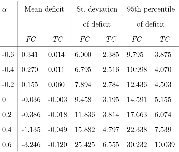
Table 6 shows that the volatility and 95th percentile of terminal deficits are smaller

in the targeted-contribution plan than in the fixed-contribution plan, for various values of

parameter α. The lag-1 autocorrelation in {δt} increases as the autoregressive parameter

α increases. (The variance of {δt} also varies withα.)

The targeted-contribution plan therefore appears to be less risky than the

fixed-contri-bution plan, even with investment returns that exhibit non-normality and serial correlation.

It is also worth highlighting that the asset allocation decision has been ignored in this

paper, for simplicity. As set out in the Introduction, we assume that the individual is

saving for a medium term of 5 years in a vehicle such as a variable-rate savings bank

account or in a low-risk mutual fund. Asset allocation becomes more important with

longer-term savings, and this is explored in detail by Campbell and Viceira (2002) among

exp µ+1₂σ2_ǫE[E[extκt _|κ

t]] = exp µ+12σ 2

ǫ 1−p+pexp µx+12σ 2

x

.The mean deficit for both fixed

and targeted-contribution plans thus decreases as σx increases in Table 5. The standard deviation and

95th percentile of deficit nevertheless increase asσx increases, highlighting the greater risk to end-wealth

α Mean deficit St. deviation 95th percentile

of deficit of deficit

FC TC FC TC FC TC

-0.6 0.341 0.014 6.000 2.385 9.795 3.875

-0.4 0.270 0.011 6.795 2.516 10.998 4.070

-0.2 0.155 0.060 7.894 2.784 12.436 4.503

0 -0.036 -0.003 9.458 3.195 14.591 5.155

0.2 -0.386 -0.018 11.836 3.814 17.663 6.074

0.4 -1.135 -0.049 15.882 4.797 22.338 7.539

0.6 -3.246 -0.120 25.425 6.555 30.232 10.039

Table 6: Mean, standard deviation and 95th percentile of terminal deficits under

fixed-contribution plan (FC) and targeted-contribution plan (TC), for various values of AR(1)

parameter α. λ1 = 0.2, λ2 = 0.01, iA= 0.4%.

others. Asset allocation depends on the individual’s coefficient of risk aversion and elasticity

of intertemporal substitution of consumption, as well as on his labor income risk and

investment horizon, and on issues such as taxation and transaction costs etc. In the

insurance and actuarial literature, asset allocation is discussed by Vigna & Haberman

(2001), Taylor (2002), Owadally & Haberman (2004), Battocchio & Menoncin (2004),

Cairns, Blake and Dowd (2006), Emms & Haberman (2008) among others.

The asset allocation decision can be incorporated in future research. It is possible to

model lifestyling portfolios, such as life-cycle or target-date funds (Shiller, 2005; Blake,

Cairns and Dowd, 2001). The method employed to adjust contributions can also be used

Implementation Issues

There are several practical investment considerations that are worth highlighting here.

First, market frictions such as taxes and transaction costs are ignored in the above, but

can be included in future simulations. Our purpose here is to model tax-free accounts

such as the TFSA (Tax-Free Savings Account) in Canada or the ISA (Individual Savings

Account) in the UK. The performance of the targeted-contribution savings plan under

the traditional and Roth IRAs (Individual Retirement Accounts) in the US, along the

lines of Adelman and Cross (2010), would be illuminating. Various related issues must be

considered in this context, namely investor behavior during the accumulation and payout

phases, reinvestment scenarios, tax rates before and after retirement, and social security.

Second, we have not explored the riskiness of the targeted-contribution plan as the

maturity T of the plan varies. Starting such a plan at different points of the economic

cycle (for example during the 1990s and 2000s) and over different horizons may produce

very different results.

Third, the targeted-contribution plan can be said to follow a contrarian investment style

in that a greater (smaller) contribution is required if the fund performs poorly (well). This

can be contrasted with the momentum style of investing. For example, if a fixed number of

units of an open-end mutual fund are bought regularly, the dollar contribution increases as

the net asset value increases. The contrarian style of the targeted-contribution plan means

that it can take advantage of investor over-reaction and market reversal effects, specially

over the long term (DeBondt and Thaler, 1985; Chopra et al., 1992). This is something

worth investigating in future work using historical data.

Finally, we investigated above whether the targeted-contribution plan performs robustly

under a range of conditions, but did not consider the optimal choice of the λ1 and λ2

utility function may be optimized for this purpose, in order to minimize end-wealth risk as

well as risk to intermediate consumption. Historical data (for example, with the bootstrap

model of the last section) and a genetic algorithm could also be used so as to minimize the

95th percentile wrt λ1 and λ2. We mention these here as items for future research.

An Application to Pension Funding

In this section, we consider a long investment horizon and we use a bootstrap stochastic

asset model resampled over 59 years of equity and bond return data. We implement

the targeted-contribution method in the funding of a defined-benefit pension plan and

investigate whether it leads to a better long-term funding position compared to a typical

actuarial funding method. It is assumed that an employer sponsors the pension plan and

pays contributions into a pension fund to provide retirement benefits to its employees.

We use the model pension plan described by Owadally (2003), except that he uses

de-terministic economic scenarios whereas we use a stochastic asset model. A key assumption

is that employees’ salaries, and also their pensions in retirement, grow in line with price

inflation. All the monetary quantities that appear below are therefore be expressed in real

terms, i.e. net of price inflation.

Pension liabilities have a simplified structure. Employees join at the age of 20. The age

profile of the pension plan membership is constant, as is the number of new entrants to the

plan every year. A pension, indexed with price inflation, is paid when employees retire at

the age of 65. Mortality follows a standard actuarial life table (English Life Table No. 12

for males). Payroll is constant in real terms and the real yearly benefit outgo is normalized

to 1. The actuarial liability is calculated at 16.94 (in real terms) using the projected unit

credit method and a real annual discount rate of 4% (McGill et al., 2004, p. 665).

long-term Treasury bonds (gilts) only. We use the bootstrap method to simulate real returns

on these assets (Efron and Tibshirani, 1993). We resample real annual returns from the

equity and gilt indices calculated by Barclays Capital (2009) from 1950 to 2008, with

income reinvested. The returns are net of price inflation, as given by the cost of living

index also calculated by Barclays Capital (2009). The pension fund portfolio is rebalanced

every year and a 60:40 equity:gilt ratio is maintained.

Annual actuarial valuations take place and the sponsor’s contributions are varied to

make up any deficit in the plan. The deficit, also known as an unfunded liability, is the

excess of the actuarial liability over assets, and a surplus is just a negative deficit. We

assume that there is no deficit initially, for example from setting up the plan or from

recent improvements to employee benefits. (That is, the initial unfunded liability is zero.

Alternatively, any initial unfunded liability could be amortized by means of a separate

schedule of payments from the plan sponsor. See for example McGillet al. (2004, p. 620).)

The pension plan actuary calculates actuarial gains and losses at yearly valuations of

the pension plan. A gain (loss) occurs if experience is more (less) favorable than was

assumed at the previous valuation (McGill et al., 2004, p. 621). We assume here that the

only source of gains and losses is the investment performance of the pension fund. That

is, all other economic and demographic factors turn out to be as assumed.

The typical actuarial practice is to amortize investment gains or losses over 5 years

(McGill et al., 2004, p. 686), which is also assumed here. If investment returns are

con-sistently lower than the investment return assumption iA made by the actuary at each

actuarial valuation, then investment losses will occur and will build up into a deficit.

Higher employer contributions are then required as these losses are amortized. Our aim

is to compare the amortization method with the targeted-contribution method given by

equation (4) (with a time unit of one year as opposed to one month).

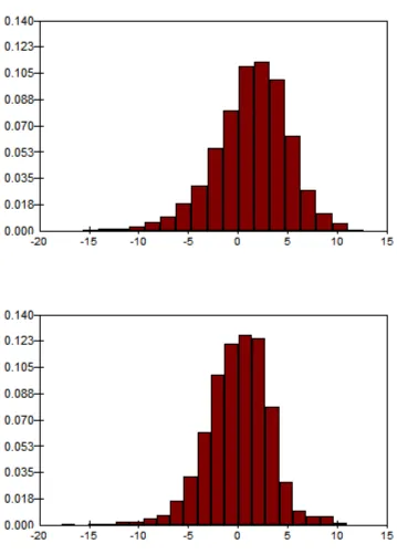
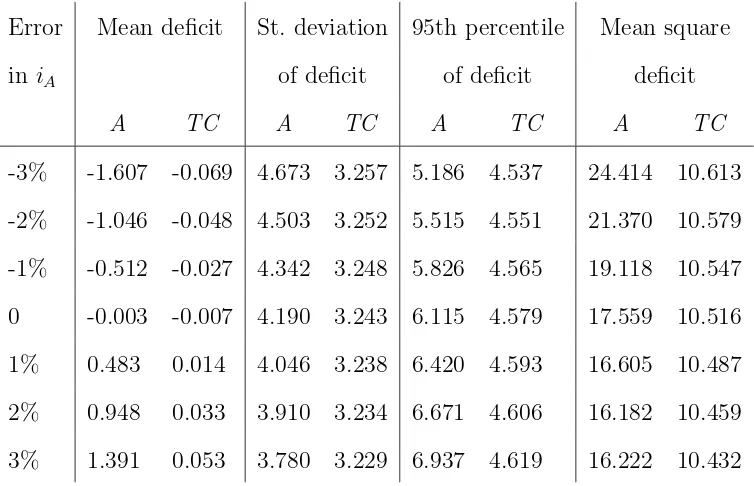
Figure 2: Histograms with identical scales for the deficit after 40 years in a pension plan

Error Mean deficit St. deviation 95th percentile Mean square

in iA of deficit of deficit deficit

A TC A TC A TC A TC

-3% -1.607 -0.069 4.673 3.257 5.186 4.537 24.414 10.613

-2% -1.046 -0.048 4.503 3.252 5.515 4.551 21.370 10.579

-1% -0.512 -0.027 4.342 3.248 5.826 4.565 19.118 10.547

0 -0.003 -0.007 4.190 3.243 6.115 4.579 17.559 10.516

1% 0.483 0.014 4.046 3.238 6.420 4.593 16.605 10.487

2% 0.948 0.033 3.910 3.234 6.671 4.606 16.182 10.459

3% 1.391 0.053 3.780 3.229 6.937 4.619 16.222 10.432

Table 7: Mean, standard deviation, mean square and 95th percentile of deficits in pension

plan after 40 years with amortization (A) and with targeted contributions (TC).

assumptioniA overstates the long-term average real return on the fund by 3% per annum.

(Using the data from Barclays Capital (2009), the pension fund makes an average annual

real return of 6.15%, so iA= 9.15% here. Parameters λ1 and λ2 in equation (4) are equal

to 0.5 and 0.03 respectively. A 40-year horizon is appropriate because employees typically

have a 40–50 year working lifetime.) The spread of deficits, and the probability of large

deficits, appear to be smaller when the targeted-contribution method is used than when

amortization is used.

Table 7 displays various statistics for the deficits under both the amortization and

the targeted-contribution method, for different errors in the investment return

assump-tion iA. The standard deviation and 95th percentile of the deficit show that the

targeted-contribution method is less risky than the amortization method in the sense that large

sen-sitive to errors in the investment return assumption, as the 95th percentile and standard

deviation do not change considerably for different investment return assumptions. This

mirrors earlier results.

Various commentators (e.g. Watson Wyatt, 2009) have noted a shift from equities to

bonds in pension fund asset allocation over the past few years. We repeated the

simula-tions above for equity:gilt allocasimula-tions of 50:50 and 40:60. The conclusions are essentially

unchanged, i.e. the targeted-contribution method results in smaller deficits and is less

sensitive to the return assumption.

The average values of the pension fund assets and contribution over 40 years are shown

in Table 8 for a 40:60 equity:gilt portfolio, which has a long-term average real return of

4.82%, and a real return assumption iA of 5.82% (so that the error in iA is 1%).

Be-cause the investment return assumption iA is too optimistic, both the amortization and

targeted-contribution methods start off with a low contribution from the employer initially.

As deficits mount in the pension fund, the targeted-contribution method demands larger

contributions more quickly than the amortization method. After 40 years, the fund levels

off at an average value of 16.92 in the targeted-contribution case and 16.45 in the

amortiza-tion case, compared to the actuarial liability value of 16.94. The average deficit is therefore

almost zero with the targeted-contribution method, whereas it is never completely removed

under amortization and a higher contribution is permanently required on average.

Note that under both methods, the pension fund is in balance after 40 years. In the

amortization case, a fund of 16.45, with contribution income of 0.24 and benefit outgo of 1,

accumulates at an investment return of 4.82% to 16.45 again after a year. In the

targeted-contribution case, a fund of 16.91, with targeted-contribution income of 0.22 and benefit outgo of 1,

accumulates at an investment return of 4.82% to 16.91 again after a year. However, the

pension fund is in balance with a nearly zero average deficit in the latter case.

lag of 10 years were not significant at 5%. Autocorrelations on real gilt returns up to lag

10 were not significant at 5%, except at lag 5. This appears to have little physical

mean-ing. Nevertheless, we also incorporated serial correlation in the simulations by resampling

using blocks of 3 years and 5 years (Efron and Tibshirani, 1993). Again, the qualitative

conclusions above are unchanged. (The detailed results are not included here to save space

and are available from the authors.)

Conclusion

We considered a savings plan where contributions are received and invested for the purpose

of meeting a given liability in the future. An example could be an investment and savings

vehicle being used to meet school or college fees in 5 years’ time. In practice, financial

advisers recommend a fixed and level regular contribution, based on an assumed investment

return on the fund. Since investment returns are random and will be different from the

assumed investment return, the fund usually undershoots or overshoots the target fund

objective, leading to a deficit or surplus respectively.

We investigated an alternative savings plan, based on a method borrowed from

in-dustrial process control and econophysics. Under this method, contributions are flexible

and are adjusted and targeted systematically so that the fund objective is met. We used

stochastic simulations to measure the risk that a terminal deficit occurs, that is, that

end-of-period wealth falls short of the target fund. The targeted-contribution method appears

to be less risky than the fixed-contribution method, in the sense that the volatility and

95th percentile of the deficit are smaller in the former case. In particular, the size of

deficits in the targeted-contribution plan is less sensitive to errors in the financial planner’s

estimate of future investment return, than in the fixed-contribution plan. These results

on contributions, with asset returns that are serially correlated, and with returns that

in-corporate large but rare market corrections and exhibit non-normality. Finally, we applied

the targeted-contribution method to a defined-benefit pension plan, with a long investment

horizon and using bootstrap resampling from actual equity and bond market data. The

standard deviation, mean square and 95th percentile of the deficit in the pension fund

were again lower with the targeted-contribution funding method than with a conventional

pension funding method.

A practical implication of this research for financial planners is that savings plans can

be designed that are more flexible for individuals. A suitable design, such as the one

described in this paper, should be not only flexible but also targeted in a systematic way

to achieve robust outcomes for individual investors.

This research can be extended in several directions, as discussed in the paper. First, the

asset allocation decision should be explored. Lifestyling portfolios can be readily included

(Shiller, 2005). The method employed to adjust contributions can also be used to adjust

asset allocation, as in Gandolfi, Sabatini and Rossolini (2007). Second, the investment

objective considered in this paper was simple and related to the end-of-period wealth only.

If the targeted-contribution plan is used for longer-term savings, such as retirement plans,

then the utility of both wealth at retirement and consumption during the accumulation

phase must be considered. Third, the choice of parameters for the targeted-contribution

plan was discussed but further work, to optimize these parameters and with back-testing

on historical data, is required. Fourth, practical considerations such as taxes and

trans-action costs can be included. Finally, the distribution of the deficit and the evolution of

Appendix: Variables λ1 and λ2

The effect of varying λ1 and λ2 on the targeted-contribution plan is considered here.

Effect on interim contributions. Tables 9 and 10 show the variance of the contributions

paid at different points in time by an investor in the targeted-contribution savings plan.

Variation withλ1 is displayed in Table 9 and variation withλ2 is in Table 10. Contributions

become more volatile as either λ1 orλ2 increases. This is a reasonable result since higher

values ofλ1 andλ2in equation (4) will magnify the effect of random deficits{Dt}, resulting

in greater variability in contribution Ct. We also illustrate this in Figure 3 which shows

three sample paths for contribution in the targeted-contribution plan, for λ2 =0, 0.01 and

0.3. As anticipated, there is more variability in the contributions required from the investor

in the targeted-contribution plan when λ2 = 0.3 than when λ2 = 0.01. When λ2 = 0.3,

contributions are briefly negative so that the investor is actually required to withdraw

monies from the fund.

For large values ofλ1andλ2, the targeted-contribution plan appears to overcompensate

for past deficits leading to large undesirable swings in contribution payments. Since

in-vestors may be unable to afford large increases in their monthly savings and contributions,

large values of λ1 and λ2 should be avoided.

Effect on end-wealth. We also investigate the effect of varying λ1 and λ2 on the risk of

a terminal deficit. Tables 11 and 12 show various statistics for the deficit at time 60, for

various values ofλ1 andλ2 respectively. Figure 4 contains a volatility surface, i.e. a plot of

the standard deviation of the terminal deficit as bothλ1 andλ2 vary. For very large values

ofλ1 andλ2 beyond those shown in Tables 11 and 12 the simulations did not converge and

near-infinite standard deviations were obtained.

The first observation that can be made is that the point at λ1 = λ2 = 0 on Figure 4

Figure 3: Sample paths of contribution in targeted-contribution plan for λ2 = 0 (bold),

λ2 = 0.01 (continuous) and λ2 = 0.3 (broken). The three sample paths correspond to the

same sample path of investment returns on the fund. F = 100,δt∼iid N(0.003792, 0.022),

iA= 0.7%, λ1 = 0.1.

even for small values ofλ1 andλ2 in the neighborhood of this point. Tables 11 and 12 bear

this out: the risk of a deficit is lower under the targeted-contribution plan than under the

fixed-contribution plan except for very large values of λ1 or λ2.

A second observation from Figure 4 is that the standard deviation of the deficit is

globally minimized at λ1 = 1 and λ2 = 0 in the targeted-contribution plan. This is also

a reasonable result since, from equation (4), this leads to Ct = C +Dt, thus requiring

the investor to make up immediately for a poor investment performance in any month by

paying off the entirety of the deficit at the beginning of the next month. Since investors

will typically wish to smooth their consumption and savings, this is a not a desirable

Third, we find that risk in the terminal deficit decreases and then increases as λ1

increases. There are minima in the standard deviation and 95th percentile of deficits in

the targeted-contribution plan at λ1 ≈1 (see Table 11). This can be explained as follows.

Suppose that returns were poor and there was a deficit in the previous month. Whenλ1 <1

(approx.), larger values of λ1 mean that larger contributions are paid at the beginning of

the current month. Deficits will therefore accumulate more slowly over successive months,

and the risk of a large terminal deficit is lower, for larger values of λ1. However, for very

large values of λ1 (when λ1 >1 approx.), the additional contribution required because of

a deficit in the previous month is larger than the deficit itself. As the contributions are fed

back into the plan, an amplification or overcompensation effect is induced and this results

in larger deficits.

A similar effect as above occurs when λ2 increases. In Table 12, the turning points

in the standard deviation and 95th percentile of deficits in the targeted-contribution plan

occur at λ2 ≈ 0.055, compared to the turning point at λ1 ≈ 1. Since λ2 acts as a tax

rate on the sum of all past deficits, whereas λ1 operates only on the latest deficit (see

equation (4)), λ2 has a larger effect on the dynamics of the plan compared to λ1, and the

amplification effect described earlier happens more readily as λ2 increases.

We also note from Figure 4 that, for large λ1, the volatility in the deficit does not

decrease asλ2 increases: it is minimized whenλ2 = 0. Again, this may be explained using

the earlier tax analogy. When the current deficit is taxed at a large enough rate λ1, even

a small tax rate λ2 on the historic sum of deficits is enough to induce overcompensation

and make deficits more volatile.

Time series analysis. We can also explain the above observations as follows. Individuals

pay Ct at time t when their investment plan is worth Ft. If they earn a log-return of δt+1

in the period (t,t+ 1), then their plan is worth

Figure 4: Plot of standard deviation (SD) of terminal deficit against λ1 and λ2. F = 100,

δt∼iid N(0.003792, 0.022),iA = 0.7%.

Under the targeted-contribution plan, the nominal deficitDtin equation (5) is the amount

by which the fund value Ft falls short of a goal or target Gt =C(1 +iA)i

−1

A ((1 +iA)t−1).

This target therefore increases every month according to

Gt+1 = (1 +iA)(Gt+C) (10)

with G0 = 0. From equations (5), (9) and (10), we find that

Dt+1 = Gt+1−Ft+1 = (1 +iA)(Gt+C) − eδt+1(Ft+Ct)

Substituting Ct from equation (4) into equation (11) gives a recurrence relation for Dt:

Dt+1 = eδt+1(1−λ1)Dt − eδt+1λ2

∞ X

j=0

Dt−j + (1 +iA−e

δt+1_)(G

t+C). (12)

{Dt} in equation (12) is a time series process with random coefficients, so analyzing

its properties is not straightforward. Instead, we resort to a comparison with a standard

linear time series process. Consider a stochastic process {Xt} that is similar to {Dt} in

equation (12) above but with non-random coefficients:

Xt+1 = (1−α1)Xt − α2

∞ X

j=0

Xt−j + Zt+1, (13)

where the random innovations or stochastic shocks {Zt} form an independent and

identi-cally distributed (i.i.d.) sequence of random variables. Differencing the above yields

Xt+1 = (1−α1+ 1−α2)Xt − (1−α1)Xt−1 + Zt+1 − Zt. (14)

{Xt} is therefore an ARMA(2, 1) time series (Hamilton, 1994). {Xt} is not invertible

because the magnitude of the coefficient of Zt in the above is not less than 1. Stationarity

depends on the coefficients of the AR part of the process. The stationarity conditions for

an AR(2) process satisfying Yt =φ1Yt−1+φ2Yt−2+Zt are: φ1 +φ2 < 1,φ2−φ1 <1 and

−1< φ2 <1 (Hamilton, 1994). Hence, {Xt} is weakly stationary if α2 >0, 2α1+α2 <4

and 0< α1 <2.

Comparing equations (12) and (13), we find that the deficit process {Dt} resembles

an ARMA(2, 1) process except that: (a) {Dt}has random coefficients, (b) its innovations

process, {(1 +iA−eδt+1)(Gt+C)}

∞

t=0, is an independent sequence if investment returns

{δt}form an independent sequence, (c) its innovations process is not identically distributed

since Gtin equation (10) is deterministic but time-varying, (d) its innovations process has

a zero mean if Eeδt

= 1 +iA, which will only hold approximately because the planner’s

The variance of a weakly stationary process (that does not start from equilibrium)

converges to a finite value as t → ∞. Notwithstanding the differences between {Dt} and

{Xt} mentioned above, the similarity that {Dt} has to an ARMA(2, 1) process may lead

us to surmise that the volatility of the terminal deficit will stabilize ifλ2 >0, 2λ1+λ2 <4

and 0< λ1 <2, approximately. Our numerical simulations are indeed consistent with this.

The simulations did not converge for {λ1 > 2, λ2 = 0.01} in Table 11, and for {λ2 >3.5,

λ1 = 0.2} in Table 12. The volatility surface in Figure 4 turns sharply upwards roughly

along the line 2λ1+λ2 = 4.

The simulations and time series analysis in this section have a practical implication for

financial planners: λ1 andλ2should not be large (sayλ1 <0.5 andλ2 <0.06) since typical

investors wish to smooth consumption and will find volatile and unstable contributions

undesirable.

References

Actuarial Foundation and WISER (2004). Seven life-defining financial decisions. The

Actuarial Foundation, Schaumburg, Illinois.

Adelman, S.W. and Cross, M.L. (2010). Comparing a traditional IRA and a Roth IRA:

theory versus practice. Risk Management and Insurance Review, 13(2), 265–277.

Akerlof, G.A. and Shiller, R.J. (2009). Animal Spirits. Princeton University Press.

Barclays Capital (2009). Equity-Gilt Study 2009. Barclays Capital, London.

Battocchio, P. and Menoncin, F. (2004). Optimal pension management in a stochastic

framework. Insurance: Mathematics and Economics, 34, 79–95.

Blake, D., Cairns, A.J.G. and Dowd, K. (2001). Pensionmetrics: stochastic pension plan

Eco-nomics, 29, 187–215.

Box, G.E.P. and Luce˜no, A. (1995). Discrete proportional-integral control with constrained

adjustment. The Statistician, Royal Statistical Society, 44(4), 479-495.

Cairns, A.J.G., Blake, D. and Dowd, K. (2006). Stochastic lifestyling: optimal dynamic

asset allocation for defined contribution pension plans. Journal of Economic Dynamics &

Control, 30, 2006, 843-877.

Campbell, J.Y. and Viceira, L.M. (2002). Strategic Asset Allocation. Oxford University

Press.

Chopra, N., Lakonishok, J. and Ritter, J.R. (1992). Measuring abnormal performance: do

stocks overreact? Journal of Financial Economics, 31, 235–268.

DeBondt, W.F.M. and Thaler, R. (1985). Does the stock market overreact? Journal of

Finance, 40, 793–805.

Efron, B. and Tibshirani, R. (1993). An Introduction to the Bootstrap. Chapman and Hall,

New York.

Emms, P. and Haberman, S. (2008). Income drawdown schemes for a defined-contribution

pension plan. Journal of Risk and Insurance, 75(3), 739-761.

Employee Benefits Security Administration. (2006). Taking the mystery out of retirement

planning. US Department of Labor.

Friesen, G.C. and Sapp, T.R.A. (2007). Mutual fund flows and investor returns: an

em-pirical examination of fund investor timing ability. Journal of Banking and Finance, 31,

2796-2816.

Gandolfi, G., Sabatini, A. and Rossolini, M. (2007). PID feedback controller used as a

tactical asset allocation technique: the GAM model. Physica A, 383, 71–78.

Kahneman, D. and Riepe, M. (1998). Aspects of investor psychology. Journal of Portfolio

Management, 24, 52–65.

Lachance, M.-E., Mitchell, O.S. and Smetters, K. (2003). Guaranteeing defined

contri-bution pensions: the option to buy back a defined benefit promise. Journal of Risk and

Insurance, 70(1), 1-16.

McGill, D.M., Brown, K.N., Haley, J.J. and Schieber, S.J. (2004). Fundamentals of Private

Pensions, 8th ed. Oxford University Press.

Owadally, M.I. (2003). Pension funding and the actuarial assumption concerning

invest-ment returns. ASTIN Bulletin, 33(2), 289–312.

Owadally, M.I. and Haberman, S. (2004). Efficient gain and loss amortization and optimal

funding in pension plans. North American Actuarial Journal, 8(1), 21–36.

Shiller, R.J. (2005). Life-cycle portfolios as government policy. The Economists’ Voice,

2(1), Article 14.

Taylor, G.C. (2002). Stochastic control of funding systems. Insurance: Mathematics and

Economics, 30, 323350.

Thaler, R.H. (1999). Mental accounting matters. Journal of Behavioral Decision Making,

12(3), 183206.

Vigna, E. and Haberman, S. (2001). Optimal investment strategy for defined contribution

pension schemes. Insurance Mathematics and Economics, 28, 233–262.

time Mean fund Mean contribution

(years) A TC A TC

0 16.9364 16.9364 0.0680 0.0680

1 16.7734 16.7734 0.1044 0.1544

2 16.6463 16.6964 0.1393 0.2001

3 16.5433 16.6597 0.1753 0.2268

4 16.4751 16.6521 0.2108 0.2391

5 16.4374 16.6539 0.2469 0.2467

6 16.4485 16.6731 0.2438 0.2450

7 16.4478 16.6844 0.2443 0.2469

8 16.4393 16.6924 0.2455 0.2502

9 16.4497 16.7183 0.2432 0.2438

10 16.4503 16.7320 0.2419 0.2431

15 16.4348 16.7877 0.2471 0.2407

20 16.4433 16.8390 0.2456 0.2328

25 16.4576 16.8750 0.2405 0.2261

30 16.4588 16.8939 0.2378 0.2240

35 16.4454 16.9007 0.2420 0.2262

40 16.4541 16.9194 0.2423 0.2209

Table 8: Mean values of fund and contribution over time in a pension plan with

time Values ofλ1

(months) 0 0.25 0.5 0.75 1 1.25 1.5 1.75

0 0 0 0 0 0 0 0 0

10 0.0004 0.0010 0.0259 0.0470 0.0784 0.1281 0.2197 0.4532

20 0.0072 0.0485 0.1127 0.2031 0.3367 0.5542 0.9709 2.0829

30 0.0354 0.1207 0.2691 0.4864 0.8149 1.3551 2.3960 5.2960

40 0.0962 0.2516 0.5456 0.9546 1.5593 2.5528 4.5084 10.1899

50 0.2051 0.4133 0.8861 1.5701 2.6174 4.3769 7.8158 17.5756

60 0.3891 0.6450 1.3724 2.4449 4.0635 6.7603 12.1910 28.3791

Table 9: Variance of contribution over time for various values of λ1 under

targeted-contribution plan. F = 100,δt∼iid N(0.003792, 0.022), iA= 0.7% and λ2 = 0.01.

time Values ofλ2

(months) 0 0.25 0.5 0.75 1 1.5 2 2.5

0 0 0 0 0 0 0 0 0

10 0.0062 0.0428 0.0843 0.1398 0.1993 0.3568 0.6269 1.1035

20 0.0308 0.2297 0.4646 0.7296 1.0452 1.8979 3.3338 6.0679

30 0.0778 0.5920 1.1826 1.9173 2.8354 5.3257 8.8990 16.4625

40 0.1611 1.2385 2.4884 3.9304 5.5867 10.1383 18.2761 32.2095

50 0.2654 2.0423 4.2115 6.7278 9.6970 18.2082 30.9891 57.3088

60 0.4151 3.1767 6.7304 10.7284 15.3809 28.7585 48.4475 87.6670

Table 10: Variance of contribution over time for various values of λ2 under

λ1 Mean deficit St. deviation 95th percentile

of deficit of deficit

FC TC FC TC FC TC

0 9.1119 0.1658 8.5931 6.5359 22.4008 10.3859

0.1 9.1119 0.5603 8.5931 4.0277 22.4008 6.9879

0.2 9.1119 0.5230 8.5931 3.1667 22.4008 5.6414

0.4 9.1119 0.4060 8.5931 2.4673 22.4008 4.3927

0.6 9.1119 0.3242 8.5931 2.1766 22.4008 3.8536

0.8 9.1119 0.2685 8.5931 2.0409 22.4008 3.5995

1 9.1119 0.2287 8.5931 1.9958 22.4008 3.4647

1.2 9.1119 0.1992 8.5931 2.0273 22.4008 3.5217

1.4 9.1119 0.1764 8.5931 2.1521 22.4008 3.7612

1.6 9.1119 0.1582 8.5931 2.4426 22.4008 4.1814

1.8 9.1119 0.1423 8.5931 3.2023 22.4008 5.3520

2 9.1119 0.1171 8.5931 9.7901 22.4008 16.1378

Table 11: Mean, standard deviation and 95th percentile of terminal deficits under

targeted-contribution plan (TC), for various values ofλ1. Fixed-contribution plan (FC) is

indepen-dent of λ1 but statistics are shown for comparison. F = 100, δt∼ iid N(0.003792, 0.022),

λ2 Mean deficit St. deviation 95th percentile

of deficit of deficit

FC TC FC TC FC TC

0 9.1119 1.3856 8.5931 3.2492 22.4008 6.5924

0.005 9.1119 0.8151 8.5931 3.1864 22.4008 5.9590

0.01 9.1119 0.5230 8.5931 3.1667 22.4008 5.6414

0.02 9.1119 0.2818 8.5931 3.1510 22.4008 5.3726

0.04 9.1119 0.1456 8.5931 3.1407 22.4008 5.1856

0.05 9.1119 0.1169 8.5931 3.1398 22.4008 5.1721

0.06 9.1119 0.0977 8.5931 3.1410 22.4008 5.1193

0.08 9.1119 0.0735 8.5931 3.1484 22.4008 5.1436

0.1 9.1119 0.0589 8.5931 3.1586 22.4008 5.0992

0.2 9.1119 0.0302 8.5931 3.2185 22.4008 5.1633

0.4 9.1119 0.0139 8.5931 3.3056 22.4008 5.3811

0.6 9.1119 0.0089 8.5931 3.4172 22.4008 5.5390

0.8 9.1119 0.0079 8.5931 3.5055 22.4008 5.6934

1 9.1119 0.0058 8.5931 3.6229 22.4008 5.8245

1.5 9.1119 0.0051 8.5931 4.0118 22.4008 6.5897

2 9.1119 0.0009 8.5931 4.6413 22.4008 7.4038

2.5 9.1119 0.0036 8.5931 5.6160 22.4008 9.0884

3 9.1119 0.0022 8.5931 7.5552 22.4008 12.4082

3.5 9.1119 -0.0722 8.5931 19.0858 22.4008 30.9285

Table 12: Mean, standard deviation and 95th percentile of terminal deficits under

targeted-contribution plan (TC), for various values ofλ2. Fixed-contribution plan (FC) is

indepen-dent of λ2 but statistics are shown for comparison. F = 100, δt∼ iid N(0.003792, 0.022),