CFD study of aquatic thrust generation by an octopus-like arm under intense prescribed deformations

Computers & Fluids 00 (2015) 1–24

& Fluids

CFD Study of Aquatic Thrust Generation by an Octopus-like Arm

1

Under Intense Prescribed Deformations

2

Asimina Kazakidi

, Dimitris P. Tsakiris

, Dionysios Angelidis

, Fotis Sotiropoulos

,

3

John A. Ekaterinaris

4

a_{Institute of Computer Science, Foundation for Research&Technology - Hellas (FORTH), 70013 Heraklion, Crete, Greece}

5

b_{St. Anthony Falls Laboratory, University of Minnesota, Minneapolis, MN, 55455-0116, USA}

6

c_{Department of Aerospace Engineering, Embry-Riddle Aeronautical University, Daytona Beach, FL, 32114, USA}

7

d_{Institute of Applied&Computational Mathematics, FORTH, 70013 Heraklion, Crete, Greece}

8

Abstract

9

The complexity in structure and locomotion of cephalopods, such as the octopus, poses difficulties in modeling and

10

simulation. Their slender arms, being highly agile and dexterous, often involve intense deformations, which are hard

11

to simulate accurately, while simultaneously ensuring numerical stability and low diffusion of the transient motion

12

results. Within the Immersed-Boundary framework, this paper focuses on an arm geometry performing prescribed

13

motions that reflect octopus locomotion. The method is compared with a Finite-Volume numerical approach to

deter-14

mine the mesh requirements that must be employed for sufficiently capturing, not only the near wall viscous flow, but

15

also the off-body vortical flow field in intense forced motions. The objective is to demonstrate and exploit the

gener-16

ality of the immersed boundary approach to complex numerical simulations of deforming geometries. Incorporation

17

of arm deformation was found to increase the output thrust of a single-arm system. It was further found that sculling

18

motion combined with arm undulations provides an effective propulsive scheme for an octopus-like arm.

19

Keywords: Computational fluid dynamics (CFD), aquatic locomotion, biological propulsion, large deformations,

20

immersed boundary method

1. Introduction

22

The appendages of cephalopods (i.e., the arms and tentacles of squids and cuttlefish, the octopus arms, and the

nau-23

tilus tentacles) are elongated muscular structures, composed of a tight 3D musculature maintaining constant volume

24

despite large deformations (termed muscular hydrostats [1]). Cephalopods may use their arms and, for squids and

cut-25

tlefish, also their fins, to perform a large repertoire of movements and behaviors [2, 3]. We are interested in

investigat-26

ing the individual role of octopus arms in aquatic locomotion and the generated hydrodynamic forces, which have not

27

been explored in detail. Studies of fish swimming (as well as of bird flight) have shown that various marine animals,

28

as well as birds, are able to exploit and control perturbations found in the surrounding fluid (e.g. vortices and eddies),

29

in order to limit the levels of energy consumption and augment the produced thrust [4, 5, 6, 7, 8, 9, 10, 11, 12, 13, 14].

30

This work aims to investigate the flow dynamics around intense octopus-like motions, in an attempt to shed light on

31

the underlying mechanisms and the energetics of cephalopod swimming.

32

The main difficulty in numerical flow simulations around time-varying geometries involving intense motions, is

33

that the computational grid must deform over time, following the motion of the body (body-fitted methods). Finite

34

volume (FV) body conforming methods include mesh deformation techniques that fulfill the geometric conservation

35

requirement [15, 16] for small deformations and can provide high-fidelity results. These methods have the advantage

36

of capturing in great detail the boundary layer around the swimming body and can simulate flows at high Reynolds

37

numbers. They also allow for a direct application of the boundary conditions on the moving body. However, the mesh

38

generation is demanding and the computational cost, for methods involving moving mesh or re-meshing strategies at

39

every time step during a simulation, can be significantly high. For large grid deformations, in particular, re-meshing

40

may affect the stability and accuracy of the numerical scheme [15].

41

Fixed-grid numerical methods, on the other hand, have attracted much attention in recent years, particularly for

42

complex fluid-structure interaction problems. The advantage of these methods is their efficiency in handling arbitrarily

43

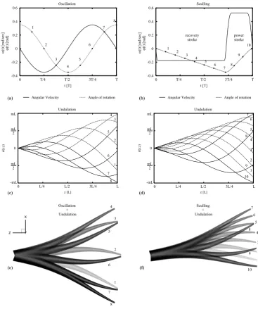
large deformations with relatively low computational cost, since no mesh-updating strategies are involved. Instead,

44

the effect of the moving body is defined on a fixed computational domain through the addition of external forces

45

in the governing equations of motion. The external force field must satisfy the no-slip condition of the fluid on the

46

moving solid body. Some of the challenges that fixed-grid methods face are related to the accurate definition of the

moving body with respect to the fixed domain, and the successful application of the boundary conditions. The

best-48

known fixed-grid numerical method for moving bodies is the immersed boundary method (IBM) of Peskin (1972)

49

[17, 18], where a delta function is implemented for the distribution of the surface forces over several mesh nodes

50

around the moving body, in order to avoid numerical instabilities. This produces smearing of the interface and, hence,

51

immersed boundary methods require increased spatial resolution around the moving body. Further developments in

52

this approach are limited to solutions with moderate Reynolds numbers [19, 20]. Approaches that overcome these

53

shortcomings are the immersed interface method (IIM) [21] and the hybrid Cartesian/immersed boundary method

54

(HCIB) [22, 23, 24, 25].

55

Here, we focused on the use of an immersed-boundary HCIB approach [24, 25] to implement and study prescribed

56

deformations, because of its robustness and handling capability. The mesh requirements for capturing the boundary

57

layer and evaluate accurately the generated hydrodynamic forces were determined by comparing the method with

58

a finite-volume approach [26, 27]. This investigation lies within a well-known field of research on aquatic animal

59

locomotion, on which there exists a considerable amount of literature [4, 5, 6, 7, 8, 9, 10, 11, 12, 13, 14, 28].

Nev-60

ertheless, many questions on aquatic swimming remain unanswered, in particular for cephalopods. This work seeks

61

to study the flow dynamics around intense octopus-like motions, utilizing computational fluid dynamic techniques on

62

time-varying arm geometries performing prescribed motions. It also aims to demonstrate and exploit the generality

63

of the immersed boundary approach to complex numerical simulations of such geometries. Incorporation of arm

de-64

formation was found to increase the output thrust of a single-arm system. It was further found that sculling motion

65

combined with arm undulation is an effective propulsive scheme for an octopus-like arm.

66

The remainder of the paper is organized as follows: Section 2 discusses the arm kinematics and the numerical

67

frameworks utilized; Section 3 presents flow simulations around an arm with and without the effect of prescribed

68

deformation; Section 4 summarizes the scopes of this study and concludes with suggestions for further work.

(b)

(a) (c)

(d)

t

Figure 1: (a-c) Snapshots of octopus swimming in an aquarium [29]. The images are superimposed with segmented

midlines of a single arm, color-coded according to the 3D arm reconstruction of (d), following the process described

in the text. (d) The 3D arm trajectories are plotted here after translation of the starting point (here the eye of the

octopus) to zero [30, 31, 32]; all dimensions are in millimetres. The plot concerns only thepower strokepart (closing

of the arms) of a more-complicated arm-swimming motion.

2. Methods

70

2.1. Octopus arm kinematics 71

Figures 1a-1c show snapshots of an octopus performing arm-swimming motion in an aquarium [29]. The images

72

also depict the topological skeleton (midline) of a single arm, after being extracted automatically, for every snapshot,

73

following the process described in detail in Yekutieli et al. [33]. Such 2D midlines can be extracted, similarly, from

74

multiple cameras, synchronized to record the motion of live octopus. Using a set of three high-definition cameras and

75

a checkerboard pattern for camera calibration [30, 31], the intrinsic and extrinsic camera parameters were estimated,

76

according to a traditional grid based calibration technique [34]. This process allows for a robust calculation of the

77

world Cartesian coordinates from the projective pinhole camera coordinates. By employing epipolar geometry

straints and least-square approximation, between each camera view, the 3D reconstruction of the medial axis of an

79

individual arm was obtained for every video frame [31, 32]. Figure 1d displays the reconstructed 3D trajectories of

80

the arm indicated in Figures 1a-1c; the trajectories are plotted after translation, such that their starting point

(corre-81

sponding, here, to the eye of the octopus) is at zero position at all times. This allows identification of the arm motion

82

separately from the motion of the animal’s body. The motion of the arm during swimming is evidently complex and,

83

therefore, such motions are in general difficult to model. However, the motion can be simplified and be broadly

char-84

acterized by a primary rotation around the starting position, and a deformation with time. Such approach is useful in

85

capturing the fundamental characteristics of complex movements and was also used in this work.

86

2.2. Arm geometry and motion approximation 87

A first attempt to model realistic movements of individual cephalopod appendages, such as the reconstructed

88

trajectories shown in Figure 1, is to consider simplified rotations of a slender octopus-like arm, around its fixed base.

89

The arm was approximated with a right circular conical frustum, of a 9.75:1 taper ratio (length, L, to base-diameter,

90

D) and a 17.5:1 aspect ratio (length to mean-diameter), for numerical simulations in quiescent fluid (Figures 2, 3). The

91

temporal variation of the angular velocityω(t) and the angle of rotationφ(t) may take various forms for a two-stroke

92

motion profile, in which the arm rotates upwards and downwards in a cyclic way. Here, we examine two basic profiles,

93

as displayed in Figures 2a, 2b: a sinusoidal oscillation, and ascullingprofile [35, 36, 37, 38] of different velocity ratio

94

βbetween a relatively slow upstroke (termed asrecovery stroke[35]) and a considerably faster downstroke (termed

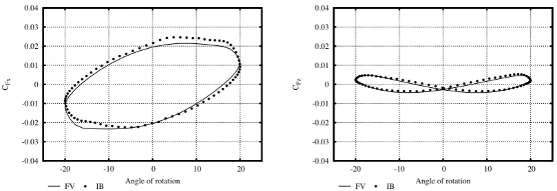
95

power stroke[35]). These motion profiles originate from observations of live octopus and analysis of the reconstructed

96

3D arm trajectories, during arm-swimming motion, in the way described in the previous paragraph and presented in

97

Figure 1. The profiles can be formulated as follows:

98

99

S culling: ω(t)=

                                                            

P1(t), 0≤t≤t1;

−ωr, t1<t≤Tr−t1;

P2(t−Tr), Tr−t1<t≤Tr+βt1;

ωp, Tr+βt1<t≤T−βt1;

P3(t−T), T−βt1<t≤T,

(2)

whereAis the amplitude of oscillation,ωr is the angular velocity of the recovery stroke (upstroke), andωp =βωr 100

is the angular velocity of the power stroke (downstroke). The timest1 = ₁₈A_ωr andTr = ₃₀61A_ωr are, respectively, those 101

required byω(t) to reach the value of−ωr, from zero, and the recovery stroke duration. The timeTp=−₅3_β(β2+60)t1 102

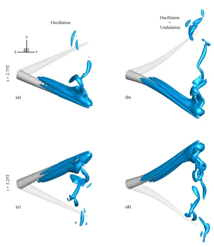
is the power stroke duration, andT is the total duration of the cyclic motion (T =Tr+Tpfor sculling). The functions 103

P1,P2,P3are 4th degree polynomials, defined such thatω(t) isC2continuous at all times and the area integral over 104

one period of the cyclic motion is zero, as follows:

105

P1(t) =−2ωr_tt₁ +2ωrt

3

t3 1

−ω_rt4

t4 1

, 0≤t≤t1;

P2(t−Tr) =2ωrt−_tTr₁ −2ωr(t −Tr)3

t3 1

−ω_r(t−Tr)4

t4 1

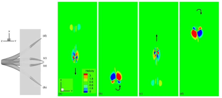
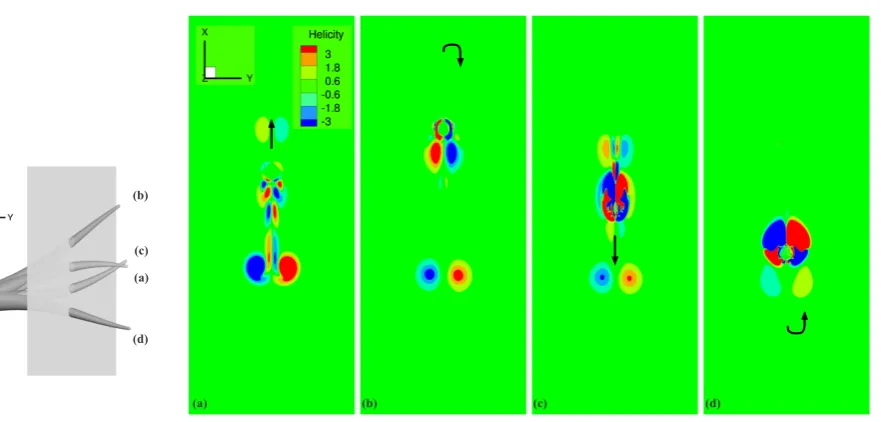
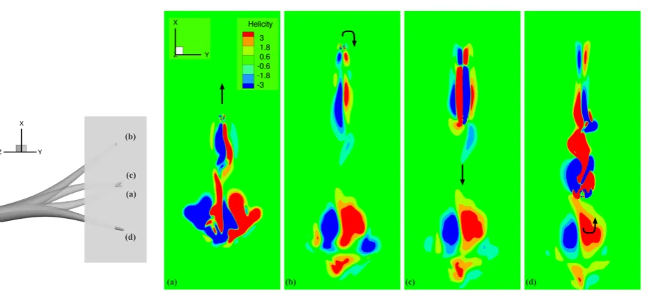
, Tr−t1<t≤Tr;

P2(t−Tr) =2ωrt−_tTr₁ −2ω3r (t−Tr)3

ω2

pt31 +

ω4 r

(t−Tr)4

ω3

pt41

, Tr <t≤Tr+βt1;

P3(t−T) =−2ωrt−t1T +2ω

3 r

(t−T)3

ω2

pt31 +

ω4 r

(t−T)4

ω3

pt41

, T −βt1 <t≤T.

(3)

In addition to purely sinusoidal and sculling rotations of the arm, we investigate the effect of prescribed arm

106

deformations [39, 40] in the form of traveling-wave undulations, which are in synchrony with the corresponding

107

rotation frequencies (Figures 2c, 2d). The time-dependent deformation is imposed in a single direction (in thex−axis),

108

that is, vertically to the longitudinal axis of the arm, according to the following function

109

d(z,t)=mz sin(2πwz−2πf{r,p}t+2πχ{r,p}), (4)

wheremis the scaled amplitude of the undulatory deformation andwis the number of wavelengths propagating along

the arm. For both the sinusoidal oscillation and sculling motions, the values ofm=0.1 andw=0.05 were assumed.

111

f{r,p}is the frequency of the traveling wave during the recovery and power strokes, respectively, andχ{r,p}is the phase 112

shift for the recovery and power strokes, respectively.

113

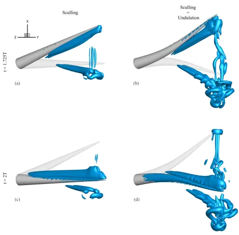
For oscillation+undulation: fr =fp= _T1, χr=χp=0.

For sculling+undulation: fr =_2Tr1 , fp=_2Tp1 , χr= Tr−2Tp

4Tr ,χp=0.25−

Tr 2Tp.

(5)

It is noted, that as a result of the unidirectional deformation, the arm elongates negligibly during the cyclic motion,

114

and the tip acquires slightly sharper edges than when undeformed (Figures 2e, 2f).

115

All numerical solutions are initiated with an undeformed arm, at rest. A sigmoid function was applied to the

defor-116

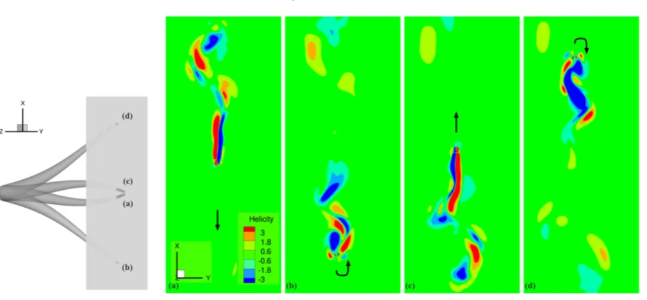
mationd(z,t) only for the first few time steps of the 1rstcycle, in order to create small increments of the deformation

117

displacement and facilitate the simulation. The expression assumed for the sigmoid was as follows

118

S(t,a,b)= 1

1+e−a(t−b), (6)

wherearepresents the growth rate andbsets the displacement of the sigmoid function along the arm’s length. For

119

both sinusoidal oscillation and sculling, the values ofa =9 andb =0.9 were chosen. S(t,a,b) was equal to 1 for

120

t>0.25T, during sinusoidal oscillation, and fort>Tr, during sculling. 121

Wake vortex topology in the simulations was visualized by theλ2 criterion, as proposed by Jeong and Hussain 122

(1995) [41], according to which, a vortex core is located at regions where the second eigenvalueλ2of theS2+Ω2tensor 123

is negative (S andΩcorrespond, respectively, to the symmetric and antisymmetric parts of the velocity gradient). The

124

helicity,H, was also used for the identification of the vortical structures. Helicity is a measure of the angle between

125

the vectors of velocity,u, and vorticity,ω =∇ ×u, defined asH =R u·ωdV[42] in volumeV, and describes the

126

topological linking and direction of rotation of vortex lines [43, 44].

-0.4 -0.2 0 0.2 0.4 0.6

0 0.7 1.4 2.1 2.8

Angle, Ang.Vel

Time

Angular Velocity Angle of rotation

ω (t ) [ra d/ se c] φ (t ) [ra d] 1 2 3 4 5 6 7 8 1 2 3 4 5 6 7 8 9 10 (f) (e) (d) (c) -1 -0.5 0 0.5 1

0 2.4375 4.875 7.3125 9.75

d(z,t) z [L] 1 2 3 4 5 6 7 8 L/4 L/2 3L/4 L 0 mL -mL mL 2 mL 2 -1 -0.5 0 0.5 1

0 2.4375 4.875 7.3125 9.75

d(z,t) z [L] 1 2 3 4 5 6 7 8 9 10 L/4 L/2 3L/4 L 0 mL -mL mL 2 mL 2 -0.4 -0.2 0 0.2 0.4 0.6

0 1.5708 3.14159 4.71239 6.28319

Angle, Ang.Vel

Time

Angular Velocity Angle of rotation

T/4 T/2 3T/4 T

0 0 T/4 T/2 3T/4 T

ω (t ) [ra d/ se c] φ (t ) [ra

d] recovery_stroke power_stroke

1 2 3 4 5 6 7 8 1 2 3 4 5 6 7 8 9 10 (b) (a) t [T] t [T] Oscillation Sculling Undulation Undulation Oscillation + Undulation Sculling + Undulation

Figure 2: (a) Sinusoidal oscillation and (b) sculling motion profiles, displaying temporal variation of angular velocity

and angle of rotation, for each case. (c-d) Time-dependent spatial deformation prescribed on the arm in the form of

wavelike undulations that match up with the corresponding frequencies of oscillation and sculling. (e) Oscillatory

rotation around the arm base combined with wavelike arm undulation of the same frequency (A=20◦_{). (f) Sculling}

rotation around the arm base combined with arm undulation in synchronized sculling frequencies, using the profiles

shown in (b) and (d) (A=10◦_{). Numerals are distinguished in left and right columns: (a), (c), (e), and (b), (d), (f). (L}

2.3. Governing equations and numerical approaches 128

A Newtonian fluid was assumed, governed by the incompressible Navier-Stokes equations [45, 46], according to

129

the following formulation

130

∂u

∂t +(u· ∇)u=−

1

ρ∇p+ν∇

2_{u, (7)}

∇ ·u=0, (8)

whereu=[u, v, w] is the velocity vector,ρis the fluid density, p is the pressure, andνis the kinematic viscosity. The

131

Reynolds number,ReD=U D/ν, is a characteristic of the flow, whereUis a velocity scale, andDis, here, the base 132

diameter of the octopus-like arm. Typical values of the Reynolds number for motions of octopus arms in seawater are

133

of the order of 1000 [47, 48]. This value (ReD=1000) was therefore adopted also in the current simulations, for a 134

Reynolds number based on the arm base diameter [49, 14].

135

Two numerical approaches were used initially (Figures 3, 4) to determine the mesh requirements that must be

136

employed for sufficiently capturing the boundary layer in the investigated forced motions: a finite volume (FV) and

137

an immersed boundary (IB) approach. The rest of the computations (Figures 5 - 11) were performed with the IB

138

approach.

139

Finite Volume (FV) framework: The FV numerical simulations were carried out with Fluent (ANSYS,

Canons-140

burg, PA) by utilizing a second-order upwind discretization scheme for momentum, a second-order pressure

dis-141

cretization scheme and the SIMPLE algorithm for pressure-velocity coupling. The ANSA (BETA CAE Systems S.A.,

142

http://www.beta-cae.gr) mesh generation package was used to construct body-fitted prismatic elements at the near wall

143

region of the arm within unstructured hybrid-type meshes. The spatial discretization around the arm was found more

144

than sufficient to numerically capture the boundary layer growth and vortex generation during the arm movement,

en-145

abling accurate evaluation of viscous flow effects. A volume mesh of 18.76x106_{tetrahedral elements was constructed} 146

in a computational domain that was 46D in thex-direction, 31D in they-direction and 20D in thez-direction; the

147

arm base was located 15D away from the upstream and lateral edges of the domain. The entire mesh rotated as a

148

solid body without deformation and a moving mesh strategy, available in the flow solver, was adopted, allowing the

high-resolution computational mesh to follow the arm at all instances of the cyclic movement. The quality and density

150

of the mesh in the near-wake field, guarantees high resolution of the near-wall region and good preservation of the

151

generated vortex patterns, with little diffusion, thus ensuring high fidelity and accuracy in our computations [14].

152

Immersed Boundary (IB) framework: The IB solution was computed using the curvilinear/immersed boundary

153

(CURVIB) method, described in detail in Gilmanov and Sotiropoulos (2005) [24] and Ge and Sotiropoulos (2007)

154

[25]. The code uses an immersed-boundary approach to solve the time-dependent, incompressible Navier-Stokes

155

equations in generalized curvilinear coordinates. The fluid domain is discretized with a background curvilinear fixed

156

grid, while the immersed body is treated as a sharp-interface boundary, discretized with an unstructured mesh. The

157

position of the immersed body is tracked and its motion is accounted for by reconstructing the solution at the IB

158

nodes in the immediate vicinity of the fluid/solid interface, using a quadratic interpolation (2nd order accurate) [24].

159

Nodes inside the solid immersed body (solid nodes) are blanked out and do not affect the solution on the fluid nodes.

160

Pressure-field boundary conditions at the IB nodes are not explicitly required because of the hybrid formulation of the

161

method [24]. Discretization in time is performed implicitly via a second-order accurate fractional step method for the

162

time integration of the governing equations.

163

The CURVIB method is coupled with the matrix-free Newton-Krylov solver, available in the PETSc library, for

164

the implicit solution of the momentum equations, and a very robust, multigrid-preconditioned GMRES solver, for the

165

solution of the pressure-correction equation [25]. The flow solver is parallelized using the MPI and PETSc libraries.

166

The background fluid mesh is parallelized by assigning a set of grid nodes to each processor using the PETSc’s

167

modules, which also manage parallel communications for structured mesh problems. The walltime per one step of

168

the simulations with the CURVIB method (e.g. for those of Section 3.4), was 0.019 hrs, for a run of 800 steps per

169

one cycle. The CURVIB method has been extensively validated and applied to a range of problems [50], e.g.

vortex-170

induced vibrations; pulsatile, physiological, transitional flow in mechanical heart valves; aquatic swimming [12, 51];

171

turbulent flow in rivers with hydraulic structures; and flows past wind turbine rotors.

172

In this study, a 20 million structured cuboid grid was used for the fluid domain of the case solved with the

173

IB method. The grid extended 30D in both the x- and z-directions and 15D in they-direction. A second,

1.5-174

times smaller domain in thez−direction was constructed with 13 million structured elements to run the preliminary

(b) (a)

Figure 3: (a) Finite-volume solution, and (b) immersed-boundary solution of an octopus-like arm performing

sinu-soidal oscillation in the xz-plane. Instantaneous iso-contours of theλ2criterion [41] showing vortex topology (λ2=

-5).

comparative studies of Figures 3a, 3b. In both grids, an inner region of size 8D x D x 2D was constructed with a

176

uniform mesh, with an element spacing ofh=0.02D, to enclose the arm tip at all instances during the cyclic motions

177

and to sufficiently capture the fine details of tip-initiated flow separation. The remaining grid was stretched towards

178

this inner region with the use of a hyperbolic tangent stretching function. The aspect ratio of the largest corner element

179

was 1.56.

180

The total hydrodynamic force,F, acting on the moving arm can be decomposed into the three Cartesian

compo-181

nents (F x,Fy,Fz), along thex,yandzdirections of the computational domain. The hydrodynamic force coefficients

182

(CF x,CFy,CFz) are defined as follows: 183

CFi=

Fi 1 2ρU

2_A (9)

wherei={x,y,z}andAis the reference area, here taken as the projected frontal area of the undeformed arm.

184

3. Results

185

3.1. Results of sinusoidal oscillation of the arm 186

A solid-body sinusoidal oscillation was examined first with both the FV and IB numerical approaches, to verify

187

the mesh requirements for sufficiently capturing the boundary layer growth around the arm. The arm rotated around

-0.04 -0.03 -0.02 -0.01 0 0.01 0.02 0.03 0.04

-20 -10 0 10 20

CFx

Angle of rotation

FV IB

-0.04 -0.03 -0.02 -0.01 0 0.01 0.02 0.03 0.04

-20 -10 0 10 20

CFz

Angle of rotation

FV IB

Figure 4: Comparison of the hydrodynamic force coefficients calculated by two numerical approaches, for an arm

performing sinusoidal oscillation in the xz-plane. The solid line is evaluated by the Finite Volume (FV) method,

whereas the dotted line by the Immersed Boundary (IB) method.

its base with a time-varying angular velocityω(t) according to Equation 1, withA=20◦(figure 3). Although small in

189

magnitude, the motion resulted in two counter-rotating vortices on the trailing sides of the arm, for each stroke. Figure

190

3 shows vortex topology at the end of the second cycle, visualized as instantaneous iso-contours of theλ2 criterion 191

(according to Jeong and Hussain, 1995 [41]). The result of Figure 3a is calculated by the finite-volume method, as

192

described in Section 2.3, and that of Figure 3b, by the immersed-boundary method, on the somewhat coarser mesh

193

(13 million elements, cf. Section 2.3). In the FV case, the computational mesh rotated together with the arm, whereas,

194

in the IB case, the background grid was fixed. The presence of two counter-rotating vortices originating from the tip

195

and extending along the lee side of the arm, at a close distance from the wall, up to about half the arm length, was

196

confirmed in both solutions.

197

The CF x and CFz force coefficients are displayed in Figures 4a, 4b, respectively, as a function of the angle of 198

rotation. Time-periodicity was achieved after about 2 periods. The results show that the force components varied

199

with the angle of rotation: for CFz, the motion produced positive thrust during upstroke and negative thrust during 200

downstroke, resulting in an effectively almost zero forward thrust in the positivez-direction (integral of the CFzcurve 201

with respect to the angle of rotation for one complete period). The solutions obtained from both the finite-volume and

202

the immersed-boundary approaches are in good agreement.

203

Figures 5a, 5c display instantaneous vortex structures, as obtained with the IB approach, from later times of the

cyclic motion at maximum amplitudes, using the finer grid (20 million elements, cf. Section 2.3). During most of this

205

solid-body sinusoidal oscillation, the angular frequency is small, reaching maximum values only for a few instances.

206

In addition, the amplitude and time duration of the motion are relatively large, allowing the vortices to diffuse between

207

recurrent upstrokes and downstrokes of the arm. Nevertheless, few seemingly non-canonical vortical structures appear

208

in the wake of the arm for both time instances presented.

209

3.2. Results of sinusoidal arm oscillation combined with arm undulation 210

The sinusoidal rotation of the arm (motion profile of Figure 2a) was subsequently combined with a wavelike

211

arm undulation, according to Equation 4 and the parameters described in Section 2.2. The time-dependent spatial

212

deformation along the arm’s length is illustrated individually in Figure 2c, in which the dashed lines correspond to the

213

upstroke (numerals from 1 to 4) and the solid lines to the downstroke (numerals from 5 to 8). The arm undulation is

214

adjusted to be in synchrony with the sinusoidal rotation of the arm; therefore, the arm acquires maximum deformation

215

at the maximum angle of rotation. As Figure 2e shows, incorporation of the undulation to the sinusoidal rotation,

216

produces considerable deformation to the arm during the cyclic motion. The figure shows the deformed arm at

217

instances where the activation functiond(z,t) is in full effect along the entire arm. Arm positions colored with light

218

gray correspond to the upstroke (numerals 1 to 4), whereas darker-colored positions correspond to the downstroke

219

(numerals 5 to 8). These positions can be tracked also in Figures 2a and 2c at the respective instances.

220

Figures 5b and 5d show vortex topology at positions of maximum arm deformation (and rotation). (It is noted that

221

thexz−plane is slightly rotated for better visualization of the vortical structures near the tip.) Two counter-rotating

222

vortices appear again in the lee side of the arm with respect to the direction of motion (upstroke and downstroke),

223

although they are deformed, following the deformation of the arm wall. These figures also display an increased

224

separation of flow from the tip, as compared to the undeformed arm at the same time instances (Figures 5a, 5c).

225

There appears to be greater flow disturbance in the region near the tip’s leeward side, shedding an extended street

226

of non-canonical vortices in the wake, of opposite helicity. The increase in the flow separation from the tip may

227

admittedly be enhanced by the unidirectional deformation that slightly distorts the tip. Nevertheless, the deformation

228

itself increases the angle of attack for a bigger section of the arm near the tip, encouraging the disturbance of flow

229

(d) (c)

(b) (a)

t = 2.75T

t = 3.25T

Oscillation Oscillation+

Undulation

Figure 5: Instantaneous near-wake vortex patterns for sinusoidal oscillation around the arm base (a, c) without and

(b, d) with arm undulations, obtained with the IB approach. Instances are shown at positions of maximum amplitude

(a-b)t=2.75T and (c-d)t=3.25T (λ2 =−1). Positions at the opposite maximum amplitude are also depicted with

light color, to indicate the direction of movement and the angular span. Note that thexz−plane is rotated for a better

(b)

(a) (c) (d)

(a) (c)

(b) (d)

Figure 6: Evolution of vortical structures visualized according to helicity, on a fixed plane near the middle of the arm,

at a distance 0.67Lfrom the arm base, for sinusoidal oscillation combined with arm undulation. (Left) Positions of the

arm with respect to the plane. (Right) Helicity contours att=(a) 1.35T (middle of upstroke, recovery), (b) 1.725T

(end of upstroke, recovery), (c) 1.85T(middle of downtroke, power), (d) 2T (end of downstroke, power). Instances in

(b) and (d) correspond to instances shown in Figures 5b and 5d, respectively. Arrows show direction of movement.

Figures 6 and 7 display the evolution of vortical structures visualized according to helicity, on fixed planes near

231

the middle of the arm, at a distance 0.67L from the arm base, and the tip of the arm, at a distance 0.93Lfrom the

232

arm base, respectively. There is considerable flow separation from the arm tip throughout the cyclic motion. Near the

233

middle of the arm, the evolution of the flow is different. The well-formed counter-rotating vortices appear to be the

234

main contributors to the generated thrust. These results are in consistent with theλ2 vortex topology of Figures 5b 235

and 5d.

236

3.3. Results of arm sculling 237

A second cyclic motion was investigated, termed assculling[52, 35, 36, 37], by adopting the motion profile of

238

Figure 2b. According to Equation 2 and the parameters described in Section 2.2, the motion is composed of a slow

239

recovery (upstroke) and fast power (downstroke). Here, the following values were assumed:A =10◦ _ω

r =10◦/sec

240

andβ=3. This motion profile was prescribed by a set of polynomial expressionsP1,P2,P3, according to Equations 241

(b)

(a) (c) (d)

(a) (c)

(b) (d)

Figure 7: Evolution of vortical structures visualized according to helicity, on a fixed plane near the tip of the arm, at

a distance 0.93Lfrom the arm base, for sinusoidal oscillation combined with arm undulation. (Left) Positions of the

arm with respect to the plane. (Right) Helicity contours att=(a) 1.35T (middle of upstroke, recovery), (b) 1.725T

(end of upstroke, recovery), (c) 1.85T(middle of downtroke, power), (d) 2T (end of downstroke, power). Instances in

(b) and (d) correspond to instances shown in Figures 5b and 5d, respectively. Arrows show direction of movement.

motion examined here involves a smaller angular span than the sinusoidal oscillation described earlier.

243

Figure 8a depicts instantaneous vortical patterns as observed at the end of the recovery stroke (at t=1.725T) and

244

Figure 8c at the end of the power stroke (at t=2T). Much like in the sinusoidal oscillation, the two counter-rotating

245

vortices at the lee side of the arm are formed during this motion too; however, they appear thinner and somewhat more

246

detached from the arm’s wall. The angular frequency has considerably large values for the duration of the sculling

247

movement, taking the value ofωr for the most part of the cycle and then reaching the maximum value ofβωr for 248

almost one quarter of the cycle. In addition, the amplitude and time duration of the overall motion are relatively small

249

(highfrandfpfrequencies). Therefore, vortical structures generated in previous cycles do not diffuse in time for the 250

subsequent upstroke and downstroke, and they continue to be visible in the flow field (vortical structures seen below

251

the arm). The speed of the motion appears to result in abrupt separation from the tip, with very little shedding in the

252

wake (as compared to the non-canonical vortices being shed during the slow sinusoidal oscillation, cf. Paragraph 3.1).

(d) (c)

(b) (a)

t = 1.725T

t = 2T

Sculling Sculling+

Undulation

Figure 8: Instantaneous near-wake vortex patterns for sculling rotation around the arm base (a, c) without and (b, d)

with arm undulations, obtained with the IB approach. Instances are shown at positions of maximum amplitude (a-b)

t=1.725 and (c-d)t=2T(λ2 =−1). Positions at the opposite maximum amplitude are also depicted with light color,

to indicate the direction of movement and the angular span. Note that thexz−plane is rotated for better visualization

of the vortical structures.

3.4. Results of arm sculling combined with arm undulation 254

The sculling rotation of the arm (motion profile of Figure 2b) was combined with a wavelike arm undulation,

(b)

(a) (c) (d)

(a) (c)

(d) (b)

Figure 9: Evolution of vortical structures visualized according to helicity, on a fixed plane near the middle of the arm,

at a distance 0.67Lfrom the arm base, for sculling combined with arm undulation. (Left) Positions of the arm with

respect to the plane. (Right) Helicity contours att=(a) 2.5T (middle of downstroke), (b) 2.75T (end of downstroke),

(c) 3T (middle of ustroke), (d) 3.25T (end of upstroke). Instances in (b) and (d) correspond to instances shown in

Figures 8b and 8d, respectively. Arrows show direction of movement.

the arm’s length is illustrated individually in Figure 2d, in which the dashed lines correspond to the recovery stroke

257

(upstroke, numerals from 1 to 7) and the solid lines to the power stroke (downstroke, numerals from 8 to 10). The

fre-258

quencies of the arm undulation during recovery and power strokes are tuned to match up with the sculling frequencies

259

(frandfp, respectively), so that maximum arm deformation is acquired at the end of each stroke. Figure 2f illustrates 260

the deformation to the arm during the sculling motion. The figure shows the deformed arm at instances where the

261

activation functiond(z,t) is in full effect along the entire arm. Arm positions colored with light gray correspond to

262

the recovery stroke (numerals 1 to 7), whereas darker-colored positions correspond to the power stroke (numerals 8 to

263

10). These positions can be tracked also in Figures 2b and 2d at the respective instances.

264

Figures 8b and 8d show vortex topology at positions of maximum arm deformation. (Note again that thexz−plane

265

is slightly rotated for better visualization of the vortical structures near the tip.) Compared to the results of Figures 5b,

266

5d, the two counter-rotating vortices in the leeward side of the arm, with respect to the direction of motion (recovery

267

and power strokes), appear to follow only loosely the deformation of the arm wall, and are more detached near the

(b)

(a) (c) (d)

(a) (c)

(d) (b)

Figure 10: Evolution of vortical structures visualized according to helicity, on a fixed plane near the tip of the arm,

at a distance 0.93Lfrom the arm base, for sculling combined with arm undulation. (Left) Positions of the arm with

respect to the plane. (Right) Helicity contours att=(a) 2.5T (middle of downstroke), (b) 2.75T (end of downstroke),

(c) 3T (middle of ustroke), (d) 3.25T (end of upstroke). Instances in (b) and (d) correspond to instances shown in

Figures 8b and 8d, respectively. Arrows show direction of movement.

tip. There is also increased separation of the flow from the tip and greater disturbance in the wake, in comparison

269

to the undeformed arm at the same time instances (left column of Figures 8). Complex vortical structures generated

270

in previous cycles do not appear to diffuse in time for the subsequent upstroke and downstroke. These structures are

271

clearly visible in the time instances displayed in Figure 8 (right column): during the upward movement of the arm

272

(Figure 8b), a small part of the large disturbed-flow structure generated in the previous cycle is drifted, while shedding

273

new structures in the wake; during the the rapid downward return of the arm (like flapping, Figure 8d), the previous

274

disturbed-flow structure is pushed further downwards.

275

Figures 9 and 10 display the evolution of vortical structures visualized according to helicity, on fixed planes near

276

the middle of the arm, at a distance 0.67Lfrom the arm base, and the tip of the arm, at a distance 0.93Lfrom the arm

277

base, respectively. There is extensive flow separation from the arm tip throughout the cyclic motion. Near the middle

278

of the arm, however, the flow disturbance is different from that of the tip. The well-formed counter-rotating vortices

279

-0.01 0 0.01 0.02 0.03 0.04 0.05 0.06 0.07

14.1372 15.708 17.2788 18.8496 20.4204

CFz

Angle of rotation

Deformed Rigid -0.01 0 0.01 0.02 0.03 0.04 0.05 0.06 0.07

0 0.7 1.4 2.1 2.8

CFz

Angle of rotation

Deformed Rigid

T/4 T/2 3T/4 T

0 0 T/4 T/2 3T/4 T

C

recovery

stroke powerstroke

C

Oscillation Sculling + Undulation Sculling

Oscillation + Undulation

P ropul si ve forc e coe ffi ci ent P ropul si ve forc e coe ffi ci ent (b) (a)

Figure 11: Temporal variation of the propulsive force coefficient, resulting from (a) oscillation and (b) sculling of the

arm around its base, either alone or combined with arm undulations. Results obtained with the IB approach.

Figures 8b and 8d.

281

4. Discussion and conclusions

282

The hydrodynamic propulsive force coefficients generated in the direction of positivez(that is, towards the arm

283

base) are shown for all four cases presented, in Figure 11. Calculated forces for pure sinusoidal oscillation and sculling

284

are displayed with dashed lines, whereas those for rotations combined with undulations are depicted with solid lines,

285

in both Figures 11a and 11b. The effect of arm undulation on the generated propulsive force is evident for both the

286

sinusoidal oscillation and sculling. In sinusoidal oscillation, the increase is almost uniform, resulting in the generation

287

of a small forward thrust (Figures 11a). In sculling, the effect is larger, particularly during the power stroke (Figures

288

11b), producing a considerably larger forward thrust.

289

Incorporation of arm deformation appears, thus, to increase the output thrust of the combined system. Indeed, a

290

single arm rotating as a solid body around its base is a single-degree-of-freedom system, with a single joint at its base.

291

This system adds some energy to the surrounding flow field in the form of the vortical structures seen in Figures 5a,

292

5c and 8a, 8c. The prescribed wavelike undulations of the arm, however, increase drastically the number of

degrees-293

of-freedom of the system, since every finite element on the arm’s surface can be thought to act as a finite joint, adding

294

extra energy to the flow field (Figures 5b, 5d and 8b, 8d); and, hence, producing extra thrust. This case differs from

a compliant arm that would deform as a result of its interaction with the flow, and would require a fluid-structure

296

interaction numerical approach to investigate.

297

We are interested specifically in the prescribed activation of the arm, that would be based on realistic octopus

298

arm kinematics (such as that of Figure 1), since octopus appendages are known to actively take part in many of the

299

observed behaviors (e.g., arm-swimming, head-up swimming, crawling, etc.). Admittedly, these movements are far

300

more complex than the simplified motion profiles we considered here. We used the immersed boundary approach in

301

order to simulate the deformation of an arm during these simplified movements and better understand the unsteady

302

hydrodynamics of the mechanism, since the extremely large deformations of the mesh required with body-fitted

303

finite-element or finite-volume approaches, are very hard to achieve even with the most advanced mesh deformation

304

techniques. It was found that the sculling motion combined with arm undulation is an effective propulsive scheme for

305

an octopus-like arm. One direction towards simulating more realistic locomotion patterns is to include translation of

306

the arm as a result of the generated propulsive force. This aspect, combined with a more accurate definition of the

307

deformation on the arm, may provide a deeper insight underlying cephalopod-like propulsive systems. Furthermore,

308

the inclusion of a second or more arms may help analyze possible interaction among different arms.

309

Aiming at a computation tool able to model intense motions, as found in aquatic locomotion instances, two

310

numerical methods were compared initially. The immersed boundary method demonstrates its suitability for handling

311

such motions. We aim to further adjust this method for special flow characteristics of time-varying geometries under

312

more complex prescribed motions.

313

Acknowledgments

314

This work was supported in part by the European Commission (EC) and the General Secretariat for Research and

315

Technology (GSRT) of the Hellenic Ministry of Education via the ESF-GSRT HYDRO-ROB Project [PE7(281)] and

316

the EC-ERDF BIOSYS-KRIPIS Project [MIS-448301 (2013SE01380036)]. Parts of these simulations were carried

317

out on the CaSToRC High-Performance Computing (HPC) system, of the LINKSCEEM/Cy-Tera resources (Project

318

pro14a108) and the PRACE Tier-1 HPC system (Project CepFlow, 12DECI0048). The authors would like to thank

319

B. Hochner, T. Flash, M. Sfakiotakis, X. Zabulis, M. Kuba, J. Oikonomidis, A. Chatzidaki, Th. Evdaimon, and S.

Stefanou, for their assistance with these studies.

321

References

322

[1] W.M. Kier, K.K. Smith, Tongues, tentacles and trunks: the biomechanics of movement in muscular-hydrostats, Zool J Linn Soc 83 (1985)

323

307–324.

324

[2] C.L. Huffard, Locomotion by abdopus aculeatus (cephalopoda: Octopodidae): Walking the line between primary and secondary defenses, J

325

Exp Biol 209 (2006) 3697–3707.

326

[3] E.J. Anderson, M.E. Demont, The mechanics of locomotion in the squid loligo pealei: locomotory function and unsteady hydrodynamics of

327

the jet and intramantle pressure, J Exp Biol 203 (2000) 2851–2863.

328

[4] M. Sfakiotakis, D.M. Lane, J.B.C. Davies, Review of fish swimming modes for aquatic locomotion, IEEE J Ocean Eng 24 (2) (1999) 237–252.

329

[5] G.V. Lauder, E.G. Drucker, Forces, fishes, and fluids: Hydrodynamic mechanisms of aquatic locomotion, Physiology 17 (2002) 235–240.

330

[6] J.C. Liao, D.N. Beal, G.V. Lauder, MS. Triantafyllou, Fish exploiting vortices decrease muscle activity, Science 302 (2003) 1566–1569.

331

[7] J.C. Liao, D.N. Beal, G.V. Lauder, M.S. Triantafyllou, The k´arm´an gait: novel body kinematics of rainbow trout swimming in a vortex street,

332

J Exp Biol 206 (2003) 1059–1073.

333

[8] E.D. Tytell, G.V. Lauder, The hydrodynamics of eel swimming. i. wake structure, J Exp Biol 207 (2004) 1825–1841.

334

[9] E.D. Tytell, The hydrodynamics of eel swimming. ii. effect of swimming speed, J Exp Biol 207 (2004) 3265–3279.

335

[10] J.O. Dabiri, S.P. Colin, J.H. Costello, Fast-swimming hydromedusae exploit velar kinematics to form an optimal vortex wake, J Exp Biol 209

336

(2006) 2025–2033.

337

[11] I.K. Bartol, P.S. Krueger, J.T. Thompson, W.J. Stewart, Swimming dynamics and propulsive efficiency of squids throughout ontogeny, Integr

338

Comp Biol 48 (6) (2008) 720–733.

339

[12] I. Borazjani, F. Sotiropoulos, Numerical investigation of the hydrodynamics of carangiform swimming in the transitional and inertial flow

340

regimes, J Exp Biol 211 (2008) 1541–1558.

341

[13] G.V. Lauder, Animal locomotion, Heidelberg, Germany, Springer-Verlag, 2010, Ch. Swimming hydrodynamics: Ten questions and the

342

technical approaches needed to resolve them, pp. 3–15.

343

[14] A. Kazakidi, V. Vavourakis, D. P. Tsakiris, J. Ekaterinaris, A numerical investigation of flow around octopus-like arms: near-wake vortex

344

patterns and force development, Comp. Meth. Biomech. Biomed. Eng. 18 (12) (2015) 1321–1339.

345

[15] P.D. Thomas, C.K. Lombard, Geometric conservation law and its application to flow computations on moving grids, AIAA Journal 17 (10)

346

(1979) 1030–1037.

347

[16] I. Demirdzic, M. Peric, Space conservation law in finite volume calculations of fluid flow, Int. J. Numer. Meth. Fluids 8 (1988) 1037–1050.

348

[17] C. Peskin, Flow pattern around heart valves: a numerical method, J Comput Phys 10 (1972) 252–271.

349

[18] C. Peskin, D. McQueen, Shared-memory parallel vector implementation of the immersed boundary method for the computation of blood flow

350

in the beating mammalian heart, J. Supercomput. 11 (1997) 213–236.

[19] D. Goldstein, R. Handler, L. Sirovich, Modeling a no-slip flow boundary with an external force field, J. Comput. Phys. 105 (1993) 354–366.

352

[20] R. Cortez, M. Minion, The blob projection method for immersed boundary problems, J. Comput. Phys. 161 (2000) 428–453.

353

[21] R. LeVeque, Z. Li, Immersed interface method for stokes flow with elastic boundaries or surface tension, SIAM J. Sci. Comput. 18 (1997)

354

709–735.

355

[22] J. Mohd-Yusof, Combined immersed boundaries/b-splines methods for simulations of flows in complex geometries. center for turbulence

356

research., Annual Research Briefs, Stanford University, NASA Ames (1997) 317–327.

357

[23] E. Fadlun, R. Verzicco, P. Orlandi, J. Mohd-Yusof, Combined immersed-boundary finite-difference methods for three-dimensional complex

358

flow simulations,, J. Comput. Phys. 161 (2000) 35–60.

359

[24] A. Gilmanov, F. Sotiropoulos, A hybrid cartesian/immersed boundary method for simulating flows with 3d, geometrically complex, moving

360

bodies, J. Comp. Phys. 207 (2005) 457–492.

361

[25] L. Ge, F. Sotiropoulos, A numerical method for solving the 3d unsteady incompressible navier–stokes equations in curvilinear domains with

362

complex immersed boundaries, J Comput Phys 225 (2007) 1782–1809.

363

[26] A. Kazakidi, D.P. Tsakiris, F. Sotiropoulos, J.A. Ekaterinaris, Numerical investigation of aquatic locomotion with cephalopod-like

ap-364

pendages, in: 19th Congr Europ Soc Biomech, (ESB2013), Patra, Greece, 2013.

365

[27] A. Kazakidi, D. P. Tsakiris, F. Sotiropoulos, J. A. Ekaterinaris, A computational fluid dynamic study of intense cephalopod-like motions, in:

366

44th AIAA Fluid Dynamics Conference, AIAA AVIATION, Atlanta, GA, USA, 2014.

367

[28] T.-H. Wu, R.-S. Guo, G.-W. He, Y.-M. Liu, D. Qi, Simulation of swimming of a flexible filament using the generalized spring

lattice-368

Boltzmann method, J Exp Biol 349 (2014) 1–11.

369

[29] A. Kazakidi, M. Kuba, A. Botvinnik, M. Sfakiotakis, T. Gutnick, S. Hanassy, G. Levy, J. A. Ekaterinaris, T. Flash, B. Hochner, D. P. Tsakiris,

370

Swimming patterns of theOctopus vulgaris, in: 22nd Annual Meeting NCM Society, Venice, Italy, 2012.

371

[30] A. Kazakidi, S. Stefanou, X. Zabulis, M. Kuba, A. Botvinnik, S. Hanassy, M. Sfakiotakis, T. Gutnick, J. A. Ekaterinaris, T. Flash, B. Hochner,

372

D. P. Tsakiris, Motion reconstruction of arm swimming in theOctopus vulgaris, in: 19th Congress of the European Society of Bioengineering

373

(ESB), Patra, Greece, 2013.

374

[31] A. Kazakidi, S. Stefanou, X. Zabulis, M. Kuba, J. A. Ekaterinaris, T. Flash, B. Hochner, D. P. Tsakiris, 3d reconstruction of octopus arm

375

swimming motion, in: 7th World Congress of Biomechanics (WCB), Boston, MA, USA, 2014.

376

[32] A. Kazakidi, X. Zabulis, D. P. Tsakiris, Vision-based 3d motion reconstruction of octopus arm swimming and comparison with an 8-arm

377

underwater robot, in: IEEE Int. Conf. Rob. Autom. (ICRA’15), Seattle, WA, USA, 2015in press.

378

[33] Y. Yekutieli, R. Mitelman, B. Hochner, T. Flash, Analyzing octopus movements using three-dimensional reconstruction, J. Neurophysiol. 98

379

(2007) 1775–1790.

380

[34] R. Y. Tsai, A versatile camera calibration technique for high-accuracy 3d machine vision metrology using off-the-shelf TV cameras and

381

lenses, IEEE Journal of Robotics and Automation 3 (4) (1987) 323–344.

382

[35] M. Sfakiotakis, A. Kazakidi, N. Pateromichelakis, D.P. Tsakiris, Octopus-inspired eight-arm robotic swimming by sculling movements, in:

383

IEEE Int Conf Rob Autom, (ICRA 2013), Karlsruhe, Germany, 2013, pp. 5135—5141.

[36] M. Sfakiotakis, A. Kazakidi, D.P. Tsakiris, Turning maneuvers of an octopus-inspired multi-arm robotic swimmer, in: 21st Med Conf Control

385

Autom, (MED’13), Chania, Greece, 2013, pp. 1343–1349.

386

[37] M. Sfakiotakis, A. Kazakidi, A. Chatzidaki, T. Evdaimon, D. P. Tsakiris, Multi-arm robotic swimming with octopus-inspired compliant web,

387

in: IEEE/RSJ Int. Conf. on Int. Rob. Syst. (IROS’14), Chicago, Illinois, USA, 2014, pp. 302–308.

388

[38] M. Sfakiotakis, A. Kazakidi, D. P. Tsakiris, Octopus-inspired multi-arm robotic swimming, Bioinspir. Biomim. (2015)in press.

389

[39] V. Vavourakis, D. Bampasakis, A. Kazakidi, N. Pateromichelakis, J.A. Ekaterinaris, D.P. Tsakiris, Generation of primitive behaviors for

390

non-linear hyperelastic octopus-inspired robotic arm, in: IEEE Int Conf Biomed Robotics Biomechatron, (BioRob) Roma, Italy, 2012, pp.

391

725–730.

392

[40] V. Vavourakis, A. Kazakidi, D.P. Tsakiris, J.A. Ekaterinaris, A nonlinear dynamic finite element approach for simulating muscular hydrostats,

393

Comput Methods Biomech Biomed Engin 17 (8) (2014) 917–931.

394

[41] J. Jeong, F. Hussain, On the identification of a vortex, J Fluid Mech 285 (1995) 69–94.

395

[42] H. Moffatt, A. Tsinober, Helicity in laminar and turbulent flow, Ann Review Fluid Mech 24 (1992) 281–312.

396

[43] D. Degani, A. Seginer, Y. Levy, Graphical visualization of vortical flows by means of helicity, AIAA Journal 28 (8) (1990) 1347–1352.

397

[44] A. Pobitzer, R. Peikert, R. Fuchs, B. Schindler, A. Kuhn, H. Theisel, K. Matkovic, H. Hauser, The state of the art in topology-based

398

visualization of unsteady flow, Computer Graphics Forum 30 (6) (2011) 1789–1811.

399

[45] G.K. Batchelor, An introduction to fluid dynamics, Cambridge University Press, 2000.

400

[46] D.J. Tritton, Physical fluid dynamics, Oxford University Press, 1988.

401

[47] Y. Gutfreund, T. Flash, Y. Yarom, G. Fiorito, I. Segev, B. Hochner, Organization of octopus arm movements: A model system for studying

402

the control of flexible arms, J Neurosc 16 (1996) 7297–7307.

403

[48] Y. Yekutieli, R. Sagiv-Zohar, R. Aharonov, Y. Engel, B. Hochner, T. Flash, Dynamic model of the octopus arm. i. biomechanics of the octopus

404

reaching movement, J Neurophysiol 94 (2) (2005) 1443–1458.

405

[49] A. Kazakidi, V. Vavourakis, N. Pateromichelakis, J.A. Ekaterinaris, D.P. Tsakiris, Hydrodynamic analysis of octopus-like robotic arms, in:

406

IEEE Int Conf Rob Autom, ICRA 2012, St Paul, Minnesota, USA, 2012, pp. 5295–5300.

407

[50] I. Borazjani, L. Ge, F. Sotiropoulos, Curvilinear immersed boundary method for simulating fluid structure interaction with complex 3d rigid

408

bodies, J Comput Phys 227 (2008) 7587–7620.

409

[51] I. Borazjani, F. Sotiropoulos, E. D. Tytell, G. V. Lauder, Hydrodynamics of the bluegill sunfish c-start escape response: three-dimensional

410

simulations and comparison with experimental data, J Exp Biol 215 (2012) 671–684.

411

[52] M. Sfakiotakis, A. Kazakidi, N. Pateromichelakis, J.A. Ekaterinaris, D.P. Tsakiris, Robotic underwater propulsion inspired by the octopus

412

multi-arm swimming, in: IEEE Int Conf Rob Autom, (ICRA 2012), St Paul, Minnesota, USA, 2012, pp. 3833–3839.