The Beta Ansatz: A Tale of Two Complex Structures

City, University of London Institutional Repository

Citation

:

This is the unspecified version of the paper.

This version of the publication may differ from the final published

version.

Permanent repository link:

Link to published version

:

Copyright and reuse:

City Research Online aims to make research

outputs of City, University of London available to a wider audience.

Copyright and Moral Rights remain with the author(s) and/or copyright

holders. URLs from City Research Online may be freely distributed and

linked to.

City Research Online: http://openaccess.city.ac.uk/ [email protected]

IMPERIAL-TP-11-AH-04, QMUL-PH-11-04

The Beta Ansatz:

A Tale of Two Complex Structures

Amihay Hanany

_{Yang-Hui He}

_{Vishnu Jejjala}

_{Jurgis Pasukonis}

Sanjaye Ramgoolam

_{and Diego Rodriguez-Gomez}

1 _{Theoretical Physics Group, The Blackett Laboratory,}

Imperial College, Prince Consort Road, London SW7 2AZ, UK

2 _{Department of Mathematics, City University, London,}

Northampton Square, London EC1V 0HB, UK;

School of Physics, NanKai University, Tianjin, 300071, P.R. China; Merton College, University of Oxford, OX14JD, UK

3 _{Department of Physics, Queen Mary, University of London,}

Mile End Road, London E1 4NS, UK

4 _{Department of Physics, Technion, Haifa, 3200, Israel;}

Department of Mathematics and Physics, University of Haifa at Oranim, Tivon, 36006, Israel

Abstract

Brane tilings, sometimes called dimer models, are a class of bipartite graphs on a torus which encode the gauge theory data of four-dimensional SCFTs dual to D3-branes probing toric Calabi–Yau threefolds. An efficient way of encoding this information exploits the theory of dessin d’enfants, expressing the structure in terms of a permutation triple, which is in turn related to a Belyi pair, namely a holomorphic map from a torus to a P1 with three

marked points. The procedure ofa-maximization, in the context of isoradial embeddings of the dimer, also associates a complex structure to the torus, determined by the R-charges in the SCFT, which can be compared with the Belyi complex structure. Algorithms for the explicit construction of the Belyi pairs are described in detail. In the case of orbifolds, these algorithms are related to the construction of covers of elliptic curves, which exploits the properties of Weierstraß elliptic functions. We present a counterexample to a previous conjecture identifying the complex structure of the Belyi curve to the complex structure associated with R-charges.

∗ _{[email protected], [email protected], [email protected], [email protected],}

[email protected], [email protected]

Contents

1 Introduction 3

2 Belyi pairs and dimer models 4

2.1 Isoradial dimers and the τR =τB conjecture . . . 8

3 Towards a general algorithm for constructing Belyi pairs 9 3.1 Belyi isx-dependent only . . . 11

3.2 The general problem . . . 13

4 Orbifolds and covering the torus 15 4.1 Unbranched covers of the torus . . . 15

4.2 Constructing unbranched covers of tori . . . 17

4.3 Example: Degree 2 covers of y2 _=x3_{+ 1 . . . . 19}

5 _C3 and its orbifolds 20 5.1 Z2×Z2 orbifolds and period doubling . . . 20

5.1.1 Double angle and a consistency check . . . 21

5.2 Degree 3 covers and dP0 . . . 21

5.3 Degree 2 covers and Z2 orbifold . . . 22

6 The conifold and its orbifolds 23 6.1 Covers and orbifolds at degree 2 . . . 23

7 Seiberg duality and τB, τR 25 7.1 The two phases of F0 . . . 25

7.2 The two phases of L222 _{and a counterexample to the τ} R =τB conjecture . . . 26

7.3 τB and τR revisited . . . 27

8 Conclusion 28

A Properties of the Weierstraß ℘-function 29

1

Introduction

The low-energy physics of D3-branes probing a toric Calabi–Yau threefold conical singularity X is given in terms of a four-dimensional conformal field theory with four supercharges. Through the AdS/CFT duality [1–3], these superconformal field theories (SCFTs) are dual to Type IIB superstring theory on AdS5 × B, where B is the base of X seen as a cone

R+× B. This is by now a well known story. Quite remarkably, these theories — including

the archetypal N = 4 super-Yang–Mills — can each be encoded in a bipartite graph drawn on a torus. This is called a dimer model or, in a more stringy language, a brane tiling [4, 5]. A nice interpretation of this graph is given in the mirror Type IIA background, as described in [6], by a so-called alga projection. Moreover, it is also possible to relate the setup to a certain fivebrane system [5,7], which generalizes the brane box [8,9] and brane diamond [10] constructions, whereby giving rise to abrane tiling. Introductions to dimer models and brane tilings may be found in the reviews [11, 12].

Of late, it was observed in [13] that dimers, regarded as a bipartite graphs on a torus T2,

can naturally be interpreted in terms of Grothendieck’s dessins d’enfants [14], or children’s drawings.∗ By labeling each edge of the dimer with a number, one encodes the data of the graph in terms of three permutation elements in the symmetric group Sd on d elements.

Here, d, which is the number of edges, corresponds to the number of fields in the dual SCFT by virtue of the standard dimer model rules. By the Riemann existence theorem (see, for example, [20]) the combinatorial data of the dimer determines a unique holomorphic mapβ (up to equivalence under holomorphic reparameterizations of the curve) from the torus T2

to P1, with branch points at{0, 1, ∞}. Henceforth, as is common in the literature but not

universal, we refer to the three special points_{0, 1, _∞}on the_P1 _{as branch points and their}

pre-images on T2, where the derivative of β vanishes, as ramification points.

Such maps have attracted much attention in the mathematical literature since, due to an important result by G. V. Belyi [21], their existence implies that the Riemann surface on which they are defined — in this case a torus — can be defined overQ, the field of algebraic

numbers. Thus theBelyi pair, consisting of (1) the Riemann surfaceT2 which is the source

of the Belyi map along with (2) the holomorphic map β, acquires a special importance. Explicit constructions of Belyi pairs are difficult, in particular due to the rigidity of the construction, which allows no moduli. Indeed, whereas ramified maps from P1 to P1 have

algorithmic methods of construction [22], Belyi maps fromT2 toP1has so far defied a general

explicit treatment [23, 24]. It was observed [13], in the context of constructing Belyi pairs associated to orbifolds of Calabi–Yaus, that an infinite series of pairs can be constructed from a “parent map” by considering the map on the n-fold unbranched cover of the original

T2. The field theory construction corresponding to orbifolds is based on [25]. The relation

between orbifolds andn-fold covers of tori has been previously observed and explored, in the

∗ _{Dessins and Belyi pairs have also appeared in string theory in the context of Seiberg–Witten curves for}

pure dimer related context, by [26–29]. In this note, we will give general constructions for the n-fold unbranched covers, and apply the constructions to give new explicit examples of Belyi pairs for small n.

In the course of exploring the meaning of the Belyi pair associated to a Calabi–Yau and associated SCFT, a first step is to explore the most basic geometrical structure associated with the Belyi pair, namely the complex structure denoted τB on the Belyi curve, which

makes the map β holomorphic. It is known that R-charges can be associated to angles of the dimer in the isoradial construction of dimers [30]. The R-charges of the SCFT, determined by a-maximization fix the structure of the dimer, hence its periodicity. This determines a complex structure on the torus which supports the dimer, denoted by τR,

which was highlighted in [13]. For the case of the conifold and C3 and their orbifolds, this

complex structure τR was shown to agree with τB. It was conjectured that this equality

holds generally.

From a physical point of view, a natural class of SCFTs to consider after orbifolds, are the other toric phases which can be reached by means of Seiberg [31], or toric, dualities [32, 33]. Below, we study such phases in the particular examples of the conifold and its orbifolds. We find that, in one case, the equalityτB =τR extends beyond its prediction by orbifolding the

conifold. However, we also find a counterexample in the context of toric phases related to orbifolds, to the conjectured equalityτB =τR. The relations betweenτBandτRare thus more

intricate and require a deeper physical explanation. In the course of these investigations, we found a proof that τR is invariant under Seiberg dualities. This forms part of a forthcoming

work [34] on invariants.

The structure of this note is as follows. In Section 2 we give a lightning review of the combinatorial description of dimers and its relation with holomorphic maps from T2 into P1. In Section 3 we discuss a general algorithm for constructing Belyi pairs. The discussion

separates a class of cases which reduces, subject to specified conditions on the structure of the dimer, to the simpler problem of Belyi maps from _P1 _to

P1 (Appendix B). In Section 4

we describe, following [13], how orbifolds are constructed in terms of the Belyi pair. Thus prepared, in Section 4.2, we introduce a general procedure to explicitly construct such covers. With this newly developed technology at hand, we study orbifolds ofC3 and the conifold in

Sections 5 and 6. Then, in Section 7 we explore different phases of the orbifolds obtained, through Seiberg duality in the field theory. In particular, we find a counterexample to the conjectured equivalence of τB and τR. We finish in Section 8 with some concluding remarks

and mention some open problems for future research.

2

Belyi pairs and dimer models

well as the recent realization that this can also be interpreted as a dessin d’enfant, and hence be encoded by a Belyi pair. A dimer model is a bipartite graph, i.e., consisting of two sets of nodes, say black and white, such that only nodes of opposite color are allowed to be connected by an undirected edge. This finite graph is then drawn on a torus, hence constituting a periodic tiling of the plane. From empirical observation of field theories, we restrict to the case ofbalanced bipartite graphs, for which we have an equal number of black and white nodes.

The dimer captures the information of the dual field theory in the following way. The faces representU(N) gauge group factors while its edges represent fields in the bifundamen-tal representation of the two faces which the edge separates. The orientation of the torus on which the graph is embedded distinguishes the fundamental representation from the antifun-damental representation. The reader may recognize this as the dual graph manifestation of a periodic quiver tiling. The advantage of the dimer model is that it also compactly encodes the superpotential. Monomial terms are formed as ordered strings of edges (fields) going, say, clockwise around white vertices and anti-clockwise around black vertices. Thereby, the superpotential is reproduced by adding together such monomials with plus sign for those originating from white nodes and a minus sign for those originating from black nodes. There is a catalog of all the known dimer models thus far, and we refer the reader to [35].

As briefly mentioned in the introduction, the dimer model can be fully encoded by a set of permutations and subsequently, by a Belyi pair, as we now recall from [13]. We first label each of the d edges with a number from 1 to d. Then, we construct a string of numbers, dubbedcycles, associated to each black node by going, say, anti-clockwise around each node. Adjoining all such cycles for each vertex gives an element, in the standard cycle notation, of the symmetric group Sd ond numbers, which we will denote asσB. By going anti-clockwise

around the white nodes we obtain the permutation elementσW. We traverse the white nodes

in the same orientation as we have traversed the black nodes.† _{We stress that both types of}

nodes are circled with the same orientation.

Therefore, we have two strings of numbers defining the cycles of permutations σB, σW in

Sd. We can naturally form a third permutationσ∞ by demanding the Calabi–Yau condition,

with multiplication in Sd, that

σB·σW ·σ∞ = 1 . (2.1)

The cycles in the third permutation σ_∞ are associated to the faces of the dimer (i.e., the gauge groups in the SCFT). We refer the reader to [13] for further details and examples.

Writing the dimer in the above language lends itself well to the interpretation of Belyi maps. First, (2.1) coincides with the relation among the homology generators on a P1

†_{We can view this prescription as traversing the edges around all the vertices according to the orientation}

of theT2 where the dimer lives. This way of constructing the permutations allows one to read off the genus

marked with three points. In fact, the set of permutations _{σB, σW, σ∞} are in one-to-one

correspondence to a unique holomorphic map β from T2 to P1 marked with three points,

say _{0,1,_∞}. This map is of degree d and is ramified over the three points, with the ramification structure given by the permutations, associated by the natural identification 0↔σB, 1↔σW, and ∞ ↔σ∞.

In this way, a cycle of length n in a permutation corresponds to a point on T2 where the

map is n-fold ramified. If the cycle originates in σB or σW, the length of the cycle is the

ramification index, which is also the number of edges that extrude from the associated black or white node. If the cycle originates inσ∞, the length of the cycle and the ramification index

correspond to one-half the number of edges that surround the associated face of the dimer. The meaning of the ramification index itself is quite simple. In terms of local coordinates w on the marked P1, which is the target of β, and local coordinates z on T2, which one

can think of as the source worldsheet, the map locally behaves as w = zn_{, where n > 1 is}

an integer. In turn, any continuous, non-self-intersecting segment on P1 connecting 0 and

1 with trivial monodromy around the point at ∞ is the image of the edges connecting the nodes in the dimer on _T2_{. Maps to}

P1 ramified over only {0,1,∞} are called Belyi maps,

and the pair of data (T2, β) is the Belyi pair. The lesson to take home is that a dimer

model (brane tiling), a permutation triple and a Belyi pair are equivalent ways of completely capturing the information of a toric quiver gauge theory.

Example of _N = 4 SYM: In order to make our discussion less abstract, let us illustrate the above concepts with the prototypical example ofN = 4 super-Yang–Mills (SYM) theory, which arises as the worldvolume theory of D3-brane transverse to the trivial non-compact toric Calabi–Yau threefold C3. This example is fully elaborated in [13].

1

1

1

1

1

1

1

1

1

1

1

1

1

1

1

1

1

1

1

1

1

1

1

1

1

1

1

1

1

1

1

1

1

1

1

1

1

1

1

1

1

1

1

1

1

1

1

1

1

1

1

1

1

1

1

2

2

1

3

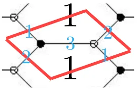
Figure 1: Dimer for the _N = 4 super-Yang–Mills theory, corresponding to the toric Calabi–Yau

threefold C3. There is only one gauge groupU(N), hence the single face, which is a hexagon marked

by1. There are three fields, all adjoints under this group, which emanate from the trivalent black/white

nodes, labeled as 1, 2, and 3. The superpotential in terms of these three fields φ1,2,3 is the standard

W = Tr(φ1φ2φ3−φ1φ3φ2), as can be seen going around the white node clockwise and the black node anticlockwise. The diagram is understood to extend doubly periodically and we have drawn, in red, the fundamental region.

fields, all adjoints in this case, and we are therefore dealing with permutations in S3. The

associated permutations can be easily read from Figure 1, which in this case are very simple:

σB = (1 2 3), σW = (1 2 3), σ∞ = (1 2 3). (2.2)

As emphasized previously, we do not reverse direction when treating black and white nodes and therefore, in our convention, we proceed anti-clockwise for both the black and white trivalent nodes, thereby giving σB and σW as above. The permutation cycle at infinity, σ∞

is obtained so that all three multiply to the identity in S3.

The explicit expression for the Belyi pair is

y2 _=x3_{+ 1 , β =} 1 +y

2 , (2.3)

where the first is the T2 written as an elliptic curve in standard form, embedded in C[x, y]

and the second is the Belyi map. Following [13], it is straightforward to verify that this pair reproduces the combinatorial data encoded by the permutations.

T2 :y2 =x3+ 1

β=1₂(1+y)

−→ P1 Local Coordinates on T2 Ramification Index of β

(0,−1) 7→β 0 (x, y)∼(,−1− 1

23) 3

(0,1) _7→β 1 (x, y)_∼(,1 + 1 2

3_{) 3}

(_∞,_∞) _7→β _∞ (x, y)_∼(−2_, −3_{) 3}

(2.4)

We can in fact make the correspondence even more explicit by looking at the pre-image underβ of the segment between 0 and 1 onP1. Because the endpoint map to the black/white

nodes by our construction, a simple non-self-intersecting curve connecting 0 and 1 with a trivial monodromy around _∞ should give precisely the edges in the dimer. Let us consider the trivial curve C(t) = t, t_∈[0, 1]. Then, the pre-image of such a segment is given by

y= 2t−1, (2.5)

on the elliptic curve y2 _=x3_{+ 1.}

In order to plot effectively, let us resort to the standard Weierstraß representation of an elliptic curve in terms of the℘-function. We recall that the℘function gives the map between the algebraic description of the torus and the description as a quotient of the complex plane modded out by a lattice (see, for example, Theorem 6.14 of [37]).

(x, y) = (℘(z;_{g2, g3}), ℘0(z;{g2, g3})) =⇒y2 = 4x3−g2x−g3 , (2.6)

Hereg2, g3 are the Weierstraß coefficients.

Indeed, for convenience, upon rescaling (x, y)_7→(4x, 4y), the Belyi curve forC3becomes

y2 _{= 4x}3 ₊ 1

16; that is, {g2, g3} = {0,− 1

16}. Thus, the explicit map from the fundamental

domain of the T2 to the interval [0,1] on the P1 is

4℘0(z, _{0,₋ 1

By numerically solving this equation for each t, we can plot in the z-plane the pre-image of the interval [0, 1] which we show in Figure 2. This is, as expected, precisely the dimer model, which, as we recall from Figure 1, lives in the fundamental region of the torus.

Figure 2: Pre-image of the interval [0,1] in the P1 by the Belyi map β explicitly recovers the dimer

model in Figure 1, a periodic honeycomb tiling of the plane for _N = 4 super-Yang-Mills theory

corre-sponding to C3.

As in [6], a projection known as the alga map, complementing the amoeba map in tropical geometry, was constructed in order to obtain the dimer model explicitly from the mirror geometry to the toric threefold. The above procedure of using the inverse of the Weierstraß ℘-function is an efficient method indeed of extracting the dimer from the associated Belyi geometry.

2.1

Isoradial dimers and the

τ

=

τ

conjecture

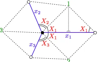
Before closing this lightning review of dimers and Belyi pairs, let us revisit the so-called iso-radial embeddingof the dimer. In [30] the concept of isoradial embedding was introduced. Following the mathematical literature (see, e.g., [38] for a review), it turns out to be highly useful to draw the dimer such that all nodes lie in circles of unit radii centered on the faces (hence the name isoradial). A fragment of such an embedding is shown in Figure 3

Figure 3: Dimer in isoradial embedding. Blue lines are edges in the tiling. Green numbers, 1, 2, and 3, are centers of tiles 1, 2, and 3, respectively. Dotted lines are all of equal length and stretched between

centers of tiles to nodes of the dimer model. Each dimer has anR-charge, e.g., the field corresponding

to the edgex1 hasR-chargeR1, then the angle X1 is π₂R1 and the angle from the center of tile 1 or

tile 2 to the end points ofx1 is π(1−R1).

are obtained through the procedure of maximizing the central charge a [39].)

We call the isoradial dimer fixed by the R-charges the R-dimer. This graph lives on a particular torus whose modular parameter is called τR. Based on a number of examples

and consistency checks, it was conjectured in [13] that the modular parameterτRisSL(2,Z)

equivalent to the modular parameterτB of the elliptic curveT2 in the Belyi pair. Although

N = 4 SYM, the conifold, and their orbifolds satisfy theτR=τB conjecture, the equivalence

turns out to be false more generally as we shall demonstrate with an explicit counterexample later in this note. However, the existence of a unique Belyi pair for each dimer, with its rich number theoretic information, motivates a deeper study of analogous number theoretic structures associated with the R-charges themselves, a theme to which we return in [34].

3

Towards a general algorithm for constructing Belyi

pairs

First, let us choose a standard form for the elliptic curve _T2_:

y2 =x(x−1)(x−λ) , j(λ) = 256(1−λ+λ

2₎3

λ2_(1−λ)2 . (3.1)

For completeness, we have also written Klein’s modular invariant j-function in terms of the λparameter. The above form emphasizes the values ofxwhereyvanishes. Another common standard (Weierstraß) formy2 _{= 4x}3_−g

2x−g3 can be obtained by an elementary coordinate

change [40].

We see immediately that in the form (3.1), there are four distinguished points on the elliptic curve: (0,0), (1,0), (λ,0), and (_∞,_∞). Let us consider the finite special pointsx0 ∈

{0,1, λ_} where y vanishes. Near the points (x0,0), our T2 will, under a linear perturbation,

look like

(x, y) = (x0+δx, δy) =⇒(δy)2 = (x0 +δx)(x0−1 +δx)(x0−λ+δx) . (3.2)

For any choice of x0 the right-hand side will be linear in δx:

(δy)2 =c δx , (3.3)

which implies that _≡ δy is a good local coordinate: (δx, δy) _∼ (2_{, ). Another special}

point is (_∞,_∞). Near this point, a good local coordinate −1 _{gives (x, y) ∼ (}−2_, −3_{). In}

addition to these distinguished points we have to be careful near the points where the first derivative ofx(x−1)(x−λ) vanishes. Locally these will look like:

y0+a δy =x0+b(δx)2 , (3.4)

which means that we must pick _≡ δx as the good local coordinate: (δx, δy) _∼ (, 2_).

Over any other point, which we shall call generic, either x or y is a good local coordinate: (δx, δy)_∼(, ).

An important difference between the four distinguished points_{(0,0),(1,0),(λ,0),(_∞,_∞)_} and other values ofxis that these other values ofxgive a pair of points (x,_±y) on the curve, whereas for the special values, there is only one point on the curve for each x.

Next, let us adopt a convenient notation, inspired by the rightmost column of (2.4), for encoding the ramification indices. Let there be W pre-images of 0, B pre-images of 1 and I pre-images of ∞; thus in the dimer there will be B black nodes, W white nodes and I polygonal faces in the fundamental domain. These equate to the number of cy-cles in the corresponding permutation. Letting the ramifications of the pre-images of the three marked points be, respectively,_{r0(1), r0(2), . . . , r0(B)},{r1(1), r1(2), . . . , r1(W)}, and

{r_∞(1), r_∞(2), . . . , r_∞(I)_}, we must therefore adjust the rational functionβ to satisfy these data. In summary, the input data of our Belyi pair will be denoted by

y2 =x(x₋1)(x₋λ) ,

  

r0(1), r0(2), . . . , r0(B)

r1(1), r1(2), . . . , r1(W)

r_∞(1), r_∞(2), . . . , r_∞(I)

 

We emphasize the constraint that P_ir0(i) = Pir1(i) = Pir∞(i), which is the degree of

the map.

Now let us proceed to our construction. We will first address the class of Belyi maps which depend only on the coordinatex. This is not as limited as one might assume upon first glance: indeed most of the maps constructed in [13], with some notable exceptions including

C3, belong to this category. We will soon unveil infinite families of examples. We will thus

address this case first before moving on to the general situation.

3.1

Belyi is

x

-dependent only

Let β(x) = P(x)/Q(x) where P and Q are polynomials in x. Thus written, the pre-images of 0 and ∞ are manifest. We may also assume, without loss of generality, that the degree of P exceeds that of Q since, after all, the reciprocal of a Belyi map is also Belyi, serving merely to shuffle the image points (0,1,_∞). We will explain in Appendix B that thex-only ansatz amounts to constructing T2 →P1 Belyi maps from P1 →P1 Belyi maps.

Let the pre-images of 0 have coordinates x = _{z1, . . . , zB0}, which we can define to be

distinct. Becauseβis assumed to have numerator of higher degree, (_∞,_∞) is always mapped to _∞, and we take all the zi to be finite. Correspondingly, the number of black nodes in

our dessin/dimer is determined as follows: each generic value zi ∈ {/ 0,1, λ} contributes two

(since, as mentioned, there would be two (square root) values of y on the elliptic curve), and each distinguished pointzi ∈ {0,1, λ}, merely one (sincey would be zero only for these

values). ThusB can be determined from B0 _{by summing with these contributions.}

Similarly, let there be I0 pre-images of ∞. Recalling that x = ∞ is always by as-sumption one of the pre-images, let us set the finite pre-images to have coordinates x = {d1, d2, . . . , dI0₋₁}, corresponding to the points where Q(x) vanishes. Again, I and I0 are

related by having double contribution from generic points and single contributions from the distinguished points.

The zeros at zi and poles at di immediately fix the factorization of the Belyi map to be

β(x) = P(x) Q(x) =

A

B0

Q

i=1

(x−zi)mi I0₋₁

Q

i=1

(x₋di)ni

, (3.6)

whereA is some overall complex number. For finite valueszi ∈ {/ 0,1, λ}, whereδx is a good

local coordinate as discussed above, the exponents mi are equal to r0(i). For distinguished

pointszi = 0,1 orλ, the good local coordinate is δy= (δx)2, so we need to divide by two to

obtain mi =r0(i)/2. Similarly, ni =r∞(i) for generic di and ni =r∞(i)/2 for distinguished

di.

factors to the product, any odd ramification index without a partner will not be taken care of by the form (3.6) and thus cannot depend on x alone. We will call such circumstances as having unpaired odd ramifications. For our prototypical example of C3, the ramification

structure, in our notation, is

  

3 3 3

 

, which is clearly odd, unpaired for all three rows. We

see indeed that here the Belyi map depends on y. A ramification structure of, for example,

  

3,3,4 3,3,4 2,2,3,3

 

is acceptable; this is an example which we will encounter later.

With the form quite explicit and the pre-images of 0 and _∞ taken care of, we must ensure that the pre-images of 1 are in accord with the data _{r1(1), r1(2), . . . , r1(W)}. One

way of doing so is to take the derivative of β(x) with respect to x and make sure that the roots of β0_{(x) vanish at a set of points, different from z}

i and di, such that the order of

vanishing upon them is in accord with the ramification indices r1(i); these will constitute

the appropriate pre-images oi of 1. In order to achieve that on top of vanishing of β0(oi) we

must also impose β(oi) = 1. In all, we have all the positions of the x-coordinates zi, di, oi

as well as the constant A to tune in order to find the Belyi map. With this input data, we can search for Belyi maps using a program such as Mathematica. We emphasize that the

input data (3.5) do not fully specify the Belyi pair and that only with the knowledge of the permutation cycles can the uniqueness theorem of Belyi apply. As we shall see later, there are significantly different dimer models which share the ramification structure.

Let us descend from the above abstraction with the illustration of a concrete example. The first phase of the theory for the Calabi–Yau cone over the zeroth Hirzebruch surface

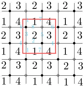
F0 ' P1 × P1 is a famous theory. The dimer for this theory is shown in Figure 4. The

ramification structure is

  

4,4 4,4 2,2,2,2

 

. Therefore, we can try β(x) = A

(x−a)4

x(x−1)(x−λ) for a, b /∈

{0,1, λ_}. We have put the points _{0,1, λ_} as zeros of the denominator by convenience since they provide three good points for infinity; this forces, naturally, that the numerator does not have such factors. A single generic factor (x−a)4 _{suffices in the numerator as x = a}

corresponds to two points on the elliptic curve.

Next, we need to solve for the critical points where β0(x) = 0, demanded by

∂xβ(x) =−

A(a₋x)3_{(a(−2(λ+ 1)x+λ+ 3x}2_{) +x(−2(λ+ 1)x+ 3λ+x}2₎₎

(x−1)2_x2_(λ−x)2 = 0 . (3.7)

Clearly, x = a would give a triple-critical points at which β itself has image 0. We also need to make sure all other critical points map to 1. One immediate way is to enforce that the second factor (a(₋2(λ+ 1)x+λ+ 3x2_{) +x(−2(λ+ 1)x+ 3λ+x}2_{)) is a perfect cubic.}

This happens, as one readily finds, when (a, λ) = (_±i,₋1), (1 2 ±

i

2, 1

2), or (1±i,2).

1

2 3

4

1

2 3

4

1

2 3

4

1

2 3

4

1

2 3

4

1

2 3

4

1

2 3

4

1

2 3

4

1

2 3

4

1 1

2 3

4 4

6 8 6

7

7 5

Figure 4: Dimer for the phase 1 ofF0.

all solutions on the same elliptic curve. In fact, these various solution are equivalent to each other by redefinitions. The solution (−i,−1) is particularly eye-catching, since this would give us the Belyi pair

y2 =x(x2−1) , β(x) = i(i+x)

4

8x(1−x2₎ , (3.8)

exactly the one given in Section C.2.3 of [13]. Thus effortlessly we can generate algorithmi-cally what once had to involve clever guesswork.

3.2

The general problem

It is tempting, given the essentially algebraic nature of our problem, to harness the power of computational algebraic geometry and computer algebra for large polynomial systems, and to develop a general method. Though in principle we can do so, as we now show, the calculations involved quickly exceeds current computer capabilities.

Nevertheless, a strategy is clear. We again start with (3.5), but now assume a form β(x, y) = P_S(₍x_x)+₎₊Q_T((_xx₎)_yy, with P, R, S, T some polynomials in x yet to be fixed. This is the most general form for the rational function β because we recall that the equation of the elliptic curve will substitute any power ofy exceeding and including the quadratic in terms of successive cubics in x. In fact, we can do better by multiplying the numerator and denominator by S(x)₋T(x)y so that the denominator becomes S(x)2 _−T(x)2_y2_{, which in}

turn is a function of x only, by substituting the y2 _{factor via the equation of the curve. In}

summary, our ansatz for the Belyi pair will take the form

(_T2_{, β(x, y)) =}

y2 _{=x(x−1)(x−λ) ,}P(x) +R(x)y

Q(x)

, (3.9)

Next, it is expedient to introduce the total derivative, which is the derivative to be henceforth used when considering the order of vanishing (i.e., ramification) at the branch points when restricted to T2. Defining F(x, y) = y2 −x(x−1)(x−λ), which must vanish

identically on the curve, we have that

d dx =

∂ ∂x −

∂xF

∂yF

∂

∂y . (3.10)

This expression is valid at the points where x is a good local coordinate. As noted before, this is not going to be the case at x0 = 0,1, λ, which is reflected in the fact that ∂yF = 2y

vanishes at these points and the second term diverges. Therefore, alternatively, we can use:

d dy =

∂ ∂y −

∂yF

∂xF

∂

∂x , (3.11)

which is valid when ∂xF 6= 0 and thus y is a good local coordinate. Finally, near the point

(_∞,_∞), where a good coordinate is with x = 1/2 _{and y = 1/}3_{, the total derivative can}

be written as

d

d =−2y ∂ ∂x −3x

2 ∂

∂y . (3.12)

If β(∞) = ∞, which is the case in our constructions, then this derivative is understood to be acting on 1/β, which is a good local coordinate in the target space.

Now that we have to specify both (x, y) we no longer have the issue with the doubling of factors mentioned in the case when β is a function of x only. Therefore, we need only adhere to a straightforward routine as follows. First, let (xi

0, yi0) be a pre-image of 0 with

ramification r0(i), this means that d

k dxk

(xi

0,y0i)

β(x, y) = 0 for all k = 0,1,2, . . . , r0(i)−1,

where k = 0 is just evaluation. This gives us r0(i) algebraic conditions, in addition to the

condition that (xi

0, yi0) needs to reside on T2. We must do this for each of the ramification

points at 0, and then at 1, for which the zeroth-order term should be set to 1. Finally, the denominator can have product form over where the map is allowed to blow up. The above was under the assumption that the pre-images are generic points. We could also repeat this, for all combinations, whenever we have an even ramification index, by demanding the vanishing of powers of the total derivative up to half of the ramification over distinguished points.

On a more optimistic note to conclude this section of the construction of Belyi pairs, we can use this aforementioned algorithm to reproduce the C3 result instantly. Starting with

the ansatz of P, R being linear in x, say, and Q being a constant suffices (recalling that (_∞,_∞) is here mapped to _∞, so there need not be any finite factors in the denominator). We can solve for the value of λ to be 1₂(1 +i√3) and β = ₂1(1 + (−1)1/4₃3/4_{y). It is easy to}

see that upon the simple coordinate transformation x0 = 1₂(3 +i√3)x−1; y0 = (−1)1/4₃3/4_y

brings the Belyi pair to the requisite form introduced in (2.3).

4

Orbifolds and covering the torus

A natural operation in string theory and in algebraic geometry is orbifolding, the identifica-tion of points by the acidentifica-tion of a finite group on a given geometrical space. When D3-branes probe an orbifolded geometry, the finite group acts on both the boundary conditions and the Chan–Paton factors of the open strings, thus giving rise to a “daughter” orbifolded theory in the fashion described in [25, 41, 42].

From the dimer perspective, orbifolding is represented in a very simple manner. As described in [4], starting from the periodic tiling corresponding to a given dimer describing the SCFT for a Calabi–Yau space, the operation of orbifolding the Calabi–Yau amounts to an enlargement of the unit cell of the tiling. This corresponds to going to an unbranched cover of the T2, which in turn has implications for the associated Belyi pairs.

4.1

Unbranched covers of the torus

We recall that the Belyi map is a branched cover from T2 to P1:

β : T2 → P1 , (4.1)

with degree d equal to the number of edges in the dimer and ramifications over _{0,1,_∞} related to the structure of the dimer. Consider now an unbranched cover Tb2 of the elliptic

curve T2:

ψ : Tb2 →T2 , (4.2)

of degree n. Such a map ψ has n inverse images for every point on _T2_{. Its derivative is}

nowhere vanishing, which is what we mean when we write that the cover is unbranched. These properties are clear from the picture of enlarging the unit cell.

The composition of β and ψ

b

β :Tb2 →P1 , where βb=β◦ψ , (4.3)

Figure 5: The composition of an unbranched cover of the torus and a Belyi map is Belyi.

coordinate z on Tb2, we have that

∂zβb=∂zβ(ψ(z)) = ∂ψβ ∂zψ , (4.4)

by application of the chain rule. Because the cover is unbranched, ∂zψ 6= 0. The only zeros

of ∂zβbtherefore occur when ∂ψβ = 0. Since β is Belyi, its derivative only vanishes at points

where β(ψ) ∈ {0,1,∞} and so βb(z) ∈ {0,1,∞} whenever ∂zβbvanishes. Thus, βb is also a

Belyi map. Consequently, we have constructed a new Belyi pair (Tb2,βb), and there should

be a corresponding dimer model.

Each ramification point of β lifts tonramification points ofβbwith the same ramification index. The number of faces of the new dimer is n times that of the original dimer. This translates into multiplying the number of factors in the gauge group by n as expected [25]. Thus, (Tb2,βb) is the Belyi pair associated to the orbifolded SCFT.

Complex structure of the cover and the τR =τB conjecture: The complex structure

of the cover Tb2 can be described as a function of the complex structure of T2. The covers

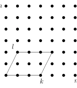
of degree n are known to be in one-to-one correspondence with integers k, p, l, such that k p = n, k, p > 0 and 0 ≤ l ≤ k−1. This is a fact from the mathematics literature, and we refer the reader to, e.g., [43]). These integers are indicated in Figure 6, with pbeing the height of the parallelogram. For each such (p, k, l), the complex structureτcover of the cover b

T2 is given in terms of the complex structure τ of the target torus T2 by

τcover(p, k, l) =

l+p τ

k . (4.5)

We note that, by construction, if the parent theory satisfies τR = τB, so, too, will the

orbifolded daughter theories. The enlargement of the unit cell determines the unit cell for the orbifold, hence τR. The cell enlargement also determines the complex structure for the

! ! ! ! ! ! ! ! ! ! ! ! ! ! ! ! ! ! ! ! ! ! ! ! ! ! ! ! ! ! ! ! ! ! ! ! ! ! ! ! ! ! ! ! ! ! ! ! ! n n k !! !! !! !! l

Figure 8: A 6-fold map of a torus with windings 3 and 2

transforml _→l+mk. Therefore the total number of inequivalent tori is

Cn=

!

k|n k−1 !

l=0

1 =!

k|n

k =!

q|n

n

q, (6.12)

wherek_|n_⇔ k divides n. The symmetry factor associated with an n-fold cover of this type is alwaysn, so the sum of the symmetry factor over all covers is given by

ξ1n,,10 = !

q|n

1

q, (6.13)

We can now calculate the leading term inW+_{(1, λA) as}

lim

N→∞W

+_{(1, λA) =} !∞

n=1 !

q|n

1 qx

n ₌ !∞ m=1 ∞ ! q=1 1 qx

mq ₌₋ !∞ m=1

ln(1−xm), (6.14)

where x= exp[₋λA/2]. Exponentiating the sum of connected maps then gives us the sum of all maps including disconnected ones. This should give the leading contribution to the QCD partition function on a torus as N → ∞.

lim

N→∞Z

+_{(1, λA) =} "

m

1

(1−xm₎ =η(x) =

!

n

p(n)xn, (6.15)

where p(n) is the number of partitions of n. This is easily seen to be identical to the QCD calculation,

Z+(1, λA) = !

n

!

R∈Yn

e−λAC2N2(R) = ! n1≥n2≥...

xn1+n2+···

#

1 +_O( 1 N)

$

(6.16)

35

Figure 6: The unit cell for a torus T2 is a drawn as a primitive lattice square. Then-fold unbranched

torusTb2 can have its unit cell being any of the lattice parallelograms marked by(p, l, k) withpk=n.

4.2

Constructing unbranched covers of tori

As we have seen, the orbifolding of a theory reduces to the construction ofn-fold unbranched covers of the torus where the parent theory Belyi map lives. In order to explicitly construct those covers, let us consider a T2 defined by an elliptic curve K which we will write in

Weierstraß form.

The Weierstraß elliptic function ℘(z;_{g2, g3}) can be used to map the description of

the torus as a quotient C/(Z(2ω1) + Z(2ω2)) by the lattice generated by (2ω1,2ω2). The

coefficients g2, g3 are functions of these half-periods ω1, ω2, which can be made explicit by

writingg2(ω1, ω2), g3(ω1, ω2). The pair

X =℘(z;g2, g3) , Y =℘0(z;g2, g3), (4.6)

where the prime denotes a derivative with respect toz, obey the equationY2 _{= 4X}3_−g 2X−

g3. The periodicities are

℘(z;g2(ω1, ω2), g3(ω1, ω3)) = ℘(z+ 2ω1;g2(ω1, ω2), g3(ω1, ω3))

= ℘(z+ 2ω2;g2(ω1, ω2), g3(ω1, ω3)) ,

(4.7)

with the same periodicities holding for℘0_(z;g

2, g3). Any even meromorphic function ofzwith

the periodicities (2ω1,2ω2) can be written as a rational function _QP(₍X_X)₎. Any odd meromorphic

function of z can be written as R_S(X_(X)Y₎ .

Let us consider now unbranched n-covers of the torus. From the point of view of the z-plane, we are considering for a given lattice, sublattices where the unit cell has n-times larger than that of the original lattice. From the cubic Weierstraß equation we are looking for the equation of the covering curve

given

y2 _{= 4x}3 _−g

2x−g3 (4.9)

and the covering map gives (x, y) as a function of (X, Y). The Weierstraß function x can be written in terms of X by summing theX at fractional arguments of the periods so as to produce the refined periodicity (see, for example, [44, 45]). It follows that the point x=_∞ maps to the point X = _∞. Using the general result that rational functions of Weierstraß functions X gives rise to all even meromorphic functions, we are led to consider

x(z) = Pn(X(z)) Qn−1(X(z))

, (4.10)

with Pn and Qn−1 being two arbitrary monic (top coefficient of the term Xn and Xn−1 is

one) polynomials of degree n and n₋1, respectively, in the variable X. This ensures that x = ∞ maps to X = ∞. Regarding the elliptic curve as an abelian group, the Weierstraß function also maps the group operation to the addition of the z-argument, so that addition theorems for Weierstraß functions give the group law. The point at infinity is the identity element since the Weierstraß function has a double pole at z = 0.

The transformation on x, (4.10), yields a transformation on y:

y(z) =x0(z) = d dz

Pn(X(z))

Qn−1(X(z))

= P˙nQn−1 −Q˙n−1Pn Q2

n−1

X0(z), (4.11)

where the dot represents x-derivative and the prime, the z-derivative. Therefore, dropping the z-dependence, we have

y= P˙nQn−1 −Q˙n−1Pn Q2

n−1

Y . (4.12)

We now have a complete description of the map from an n-fold cover to the torus, in terms of the affine coordinates in Weierstraß form, namely equations (4.10) and (4.12). Substituting these into the original curve in (2.6) and simplifying, we find that

Y2 = 4P

3

nQn−1−g2PnQ3n−1−g3Q4n−1

˙

PnQn−1 −Q˙n−1Pn

2 , (4.13)

as the affine equation of the unbranchedn-fold covering torus. Imposing the Weierstraß form

4P3

nQn−1−g2PnQ3n−1−g3Q4n−1

˙

PnQn−1−Q˙n−1Pn

2 = 4X

3_−G

2X−G3 (4.14)

for some new coefficients (G2, G3). In other words, we need to solve identically in x, that

4P_n3Qn−1−g2PnQ3n−1−g3Q4n−1−

4X3−G2X−G3 P˙nQn−1−Q˙n−1Pn

2

The left-hand side is a polynomial in X of degree 4n₋1. Since the above equation must hold for arbitrary X, it must be that the 4n coefficients of the left-hand side vanish. On the other hand, the meromorphic transformation of (X, Y) was expressed in terms of the Pn, Qn−1 polynomials. Also, as the coefficient of the highest power is one, these polynomials

involve n and n−1 a priori unknown constants, respectively. Finally, since we also need to fix (G2, G3), in fact our transformation involves 2n+ 1 unknowns. The 4n equations form

an over-complete system. However, we are guaranteed the existence of multiple solutions since we know that the counting of inequivalent coverings of tori, which are given by integers [k, l, p] obeyingkl=n;k, l >0,0_≤l _≤k₋1 [26–29]. The precise matching of the solutions of the polynomial equation (4.15) with the [k, l, p] data is not trivial. It will be given in examples for smalln in the following.

The above discussion in terms of polynomials Pn(X), Qn−1(X) is adequate for

computa-tions, and is similar in complexity to our constructions for general Belyi maps from torus in Section 3. Further uses of the beautiful theory of Weierstraß functions allow somewhat more explicit algorithms studied under the heading of transformation theory of elliptic func-tions and modular relafunc-tions, e.g [44]. Most of the key formulae, such as those for fractional modifications of a period, integer multiplication of thezargument, are collected in [45]. Nev-ertheless completely explicit general formulae for the polynomials at generaln matched with covering space data [k, l, p] remain elusive enough to have a role in cryptography (see, for example, [46] for improved algorithms and for references to the literature on applications). In the following, we work out some examples using the direct method described above. In an appendix, we describe some key equations and applications from the elegant method of [44].

4.3

Example: Degree

2

covers of

y

=

x

+ 1

Consider the particular case of our familiar example y2 _{= x}3 _{+ 1. Following the above}

prescription, the transformation corresponding to degree two covers (at most quadratic in the numerator of (4.10)) must be

(x, y) =

X2_+α

1X+α0

X+β0

, X

2_{+ 2β}

0X+ (α1β0−α0)

(X+β0)2

Y

. (4.16)

Upon substituting this generic form in the curve equation and specializing to the case (4.15), we find a number of different solutions in addition to the trivial one.

Solving for the coefficients, we see that there are three non-trivial transformations:

(x, y) =

3ω2n_{+ 8ω}−2n_X−16X2

8 (ω−2n_−2X) ,

X2_{−X ω}−2n₊ 7 16ω

2n

(X− 1

2ω−2n)2

Y

, (4.17)

with

These give us the possible covering solutions

Y2 =X3₋ 15 16ω

2n_X+11

32 . (4.19)

Using the standard formula,

j = 1728 g

3 2

g3

2−27g32

, (4.20)

we see that this curve has j-invariant 54000. On the other hand, the original curve had vanishing j-invariant, which corresponds to τ =eiπ3. For a degree two cover with [k, l, p] = [1,2,0] from Figure 6, we expectτ to becomeτcover = 2τ = 2ei

π

3. Indeed, one can check that

j(τcover) = 54000. Since the Klein j-invariant classifies equivalence classes of elliptic curves,

we have indeed arrived at the correct one.

5

_C

and its orbifolds

Following the above discussion of constructing Belyi pairs and extracting n-fold covers, we now turn to concrete examples. Again, let us begin with our familiar C3, whose Belyi

pair we recall from equation (2.3). We construct various Abelian orbifolds by following the technology developed above.

5.1

_Z

_×

_Z

orbifolds and period doubling

Let us start with examining the_Z2×Z2 orbifold of C3. Since the degree of the cover is four,

we should consider the transformation

x = X

4_+α

3X3+α2X2+α1X+α0

X3_+β

2X2+β1X+β0

, (5.1)

as well as a corresponding expression for y. Plugging these into (4.15), we can find all the solutions. After some algebra, we deduce that

(x, y) =

8X(₋1 + 8X3₎

(1 + 64X3₎ ,

8 (₋1 + 160X3_{+ 512X}6₎

(1 + 64X3₎2 Y

, (5.2)

with the resulting Belyi pair:

Y2 =X3+ 1

64 , β =

(Y + 3)3_{(Y −1)}

16Y3 . (5.3)

One can easily check, has the correct combinatorial data for the expectedC3/Z2×Z2, namely

by checking the order of vanishing at the pre-images of 0,1 and _∞, its ramification structure

is precisely

  

3,3,3,3 3,3,3,3 3,3,3,3

5.1.1 Double angle and a consistency check

We can cross check our result by noting that theZ2×Z2 orbifolding amounts to a doubling

the unit cell in the two directions in the complex plane. This procedure is a classical one known as doubling the period, and our transformation must thereby be realized. This is the reason why we have chosen the Z2 ×Z2 orbifold as our initial example. Recalling that our

Weierstraß curve

¯

y2 _{= 4 ¯x}3_−g

2x¯−g3 (5.4)

has (¯x,y¯) = (℘(z), ℘0_{(z)). Applying the period-doubling formula [45] for the ℘-function:}

℘(2z) =

℘(z)2 ₊g2

4 2

+ 2g3℘(z)

4℘(z)3_−g

2℘(z)−g3

; (5.5)

hence, in terms of the x, this is the transformation

¯ x =

¯ X2₊g2

4 2

+ 2g3X¯

4 ¯X3_−g

2X¯ −g3

. (5.6)

To get rid of the coefficient 4 in front of the ¯x, let us call ¯y = √y

2 and ¯x =

x

2, so that

the curve looks like y2 _=x3_−g

2x¯−2g3, while the transformation is x = 1₄ (X

2_+g

2)2+16g3X

X3_−g2X−2g3 . Applying (5.6) to our C3 example withg2 = 0 andg3 = 1 gives us

(x, y) =

X(X3₋₈₎

4 (X3_{+ 1)},

−8 + 20X3_+X6

8 (X3_{+ 1)}2 Y

(5.7)

It is straightforward to check that this leaves invariant the curve. It should then correspond to doubling the unit cell in the two directions, such that theτ remains unchanged. Finally, upon rescaling (X, Y) 7→ (X₄, Y₈) in our transformation (5.2), we recover exactly the map (5.7). In other words, the four-fold cover is indeed consistent with the period doubling.

5.2

Degree

3

covers and

dP

Emboldened by our success, we can move on to further orbifolds. The most famous one is undoubtedly the _Z3 orbifold of C3, otherwise known as the Calabi–Yau cone dP0 over the

zeroth del Pezzo surface, which is simply the complex projective plane. As the degree is three, we should consider

x = X

3_+α

2X2+α1X+α0

X2_+β

1X+β0

(5.8)

along with the corresponding expression fory. Clearly, there are various degree three covers, depending on how the unit cell is enlarged. We would like however to find dP0, which

Thus, plugging the above transformation into (4.15) and imposing that we want covers with the same τ, we easily find

(x, y) =

X3₋₄

27X2 ,

27X3_{+ 8}

27X3 Y

, (5.9)

giving the curve

Y2 =X3₋ 1

27 . (5.10)

It is easily checked that the rescaling (X, Y)7→(−X

3,

i

3√3Y) gives us the Belyi pair:

Y2 =X3+ 1 β=

i

6√3Y 3₊Y2

2 −

i√3 2 Y −

1 2

(Y −1)(Y + 1) , (5.11)

which can be shown to yield to the correct ramification structure

  

3,3,3 3,3,3 3,3,3

 

. Furthermore,

this Belyi pair was previously constructed in [13], and we reproduce this result.

5.3

Degree

2

covers and

_Z

orbifold

Let us finally construct the cover corresponding to the Z2 orbifold of C3, or more precisely, C2/Z2×C. This is especially interesting, as the corresponding field theory is theA1 N = 2

SCFT. Applying the results from Section 4.3, the appropriate transformation is

(x, y) =

3 + 8X−16X2 8 (1−2X) ,

X2_−X+ 7 16

(X₋1 2)2

Y

, (5.12)

and the resulting curve is Y2 _=X3₋ 15 16X+

11 32.

Substituting the transformation rule into the Belyi map for C3 yields the Belyi pair:

Y2 =X3− 15 16X+

11

32 , β =

1 2

1 + X

2_−X+ 7 16

(X− 1 2)2

Y

. (5.13)

Again, we can easily check, by finding the order of vanishing at the critical points of map,

that the ramification structure is

  

3,3 3,3 3,3

 

, which is indeed as expected for C 2_/

Z2×C.

This concludes our treatment of the orbifolds of C3, and we see a consistent and

6

The conifold and its orbifolds

To exhibit the general applicability of our methodology, we consider other Calabi–Yaus. The second most famous theory, after C3, in the AdS/CFT dictionary, is arguably the conifold

theory.

From [13] we recall that its Belyi pair is:

y2 =x3−x , β = (x+ 1)

2

4x , (6.1)

with ramification structure

  

4 4 2,2

 

. Incit. ibid., also the phase I of the chiralZ2 orbifold

of the conifold, namelyFI0, the first toric phase of the cone over the zeroth Hirzebruch surface,

was found. The corresponding pair was already presented in our case study in equation (3.8), and we recall them here as:

y2 _=x3 _{−x , β}

I =i

(i+x)4

8x(1−x2₎ . (6.2)

It is easy to see that the following transformation takes the conifold pair into theFI0 one:

(x, y) _7→

2ix

−1 +x2,

√

2ei3π/4 1 +x

2

(1₋x2₎2 y

. (6.3)

We can further check this transformation by noting that acting twice thereby produces a doubling of the periods, and thus we can apply and compare with the standard double angle formulae. For the conifold case we have g2 = 1 , g3 = 0 so

x 7→ 1 4

(x2_{+ 1)}2

x3_−x (6.4)

On the other hand, if we act two times with our transformation, we find

x _7→ 4 x

3_−x

(x2_{+ 1)}2 (6.5)

However, in the conifold case an automorphism of the pair isx7→1/x, so this transformation in fact coincides with the one coming from the double angle formulae.

6.1

Covers and orbifolds at degree

2

Our ansatz for the transformation is:

(x, y) =

X2_+α

1X+α0

X+β0

, X

2_{+ 2β}

0X+ (α1β0−α0)

(X+β0)2

Y

. (6.6)

Upon substitution into (4.15) we find essentially two classes of non-trivial solutions below:

1. Recovering _F0:

The first such solution is

(x, y) =

4X2_{+ 1}

4X ,

4X2₋₁

4X2 Y

(6.7)

which takes the curve into Y2 _=X3₊X

4. Defining the coordinate change

(X, Y) _7→

i(1 +X) 2 (X₋1),

i−1 2 (X₋1)2 Y

, (6.8)

one can easily check that the curve goes to the desired Y2 _{= X}3 _{− X while the}

transformation becomes the expected result in (6.3).

2. Another _Z2 cover

The solution yielding to FI0 is not the only one. In fact, it is straightforward to check

that the following transformation‡ _{is also a solution of our general set of equations for}

degree two covers

(x, y) =

(1 + 4X)2

8 (1 + 2X),

X2_+X+ 3 16

(X+ 1₂)2 Y

. (6.9)

The resulting curve isY2 _=X3₋11 16X−

7

32 and it is immediate to check thatj = 287496.

On the other hand, this Z2 cover should correspond to enlarging the unit cell in one

direction. That should correspond toτ _→2τ. The original curve hadj-invariant 1728, which corresponds to τ =i and hence a square unit cell. Thus, we should expect the enlarged unit cellZ2 cover to have j =j(2i), which in fact is the expected 287496.

We have constructed the cover corresponding to a non-chiral Z2 orbifold of the

coni-fold.§

We can now plug this into the original conifold Belyi map and find that for this _Z2

orbifold and find the Belyi pair to be

Y2 =X3 −11 16 −

7

32 , βII =

(3 + 4X)4

32 (1 + 2X) (1 + 4X)2 . (6.10)

‡_{There is yet another solution with the same properties as this one. It should be related to enlarging the}

unit cell along the other direction.

§ _{Note that, as expected, when thought from a generic point of view as described in the first section, the}

After some computation, one can check that this is a Belyi map, with ramification

structure

  

4,4 4,4 2,2,2,2

 

. This has the correct properties for C/Z2, a space to which

one is commonly referred asL222_{. In fact, the map above corresponds to the first toric}

phase of such a theory, as we will discuss momentarily.

7

Seiberg duality and

τ

, τ

As first noted in [32, 33], typically for a given Calabi–Yau singularity more than a single dual gauge theory can be found. Such different “phases,” dubbed toric phases, are in fact connected by Seiberg duality. It is thus very natural to ask how Seiberg duality arises in the context of the Belyi construction. To this end, we continue the Z2 examples of the conifold

described in the last section and we show the Belyi pairs for the corresponding Seiberg dual phases.

7.1

The two phases of

_F

It is by now well known that the cone over the zeroth Hirzebruch surface F0 has two toric

Seiberg dual pairs, which we will denote by F0(I) and F0(II). The Belyi pair for F0(I)

was already presented in (6.2). The second phase has ramification structure

  

3,3,3,3 3,3,3,3 2,2,4,4

  ,

which conveniently falls into the category of the absence of unpaired odd indices, and can thus be readily treated by the x-only beta ansatz. We find the Belyi pair to be

y2 =x3−x , βII =i

(x2₋₍₋₁₎1/3₎3

3√3x2_(x2₋₁₎ . (7.1)

In fact, armed with the method of explicitly drawing the dimer from the Belyi map using the inverse Weierstraß function as expounded in (2.6), we can readily check this map by drawing the pre-image of the [0, 1] segment, which in this case must be done fully numerically. The result is shown in Figure 7.

It is easy to construct and compute the τR of the isoradial dimer, which is τR = i. On

the other hand, from the pair above it is easy to see that in factτB =i, thus also satisfying

τB =τR. We stress that this does not follow automatically, as phase II is not obtained by

constructing a double cover of the parent theory, as is the case for phase I.

We also note that τR is the same in both Seiberg dual phases. In fact, this is a general

Figure 7: Pre-image of the interval [0,1], drawn by numerically inverting the Weierstraß function,

explicitly recovers the F0(II) dimer from the Belyi pair in (7.1).

7.2

The two phases of

L

and a counterexample to the

τ

=

τ

conjecture

The first phase of the non-chiral Z2 orbifold of the conifold L222 was described in (6.10).

There is also a Seiberg dual phase of the geometry. For the dimer models of these theories,

we again refer the reader to [35]. This second phase has the ramification data

  

3,3,4 3,3,4 2,2,3,3

  

and once more luckily falls into the x-only beta ansatz. We thus readily arrive at the quite non-trivial Belyi pair:

y2 _{=x(x−1)(x−(8(−20−9}√₅₎₎−1_{), β =} 25x2(−5 + 5

√

5 + 16x)3

8(−5 + 2√5 + 10x)3_{(−20 + 9}√_{5 + 40x)} .

(7.2) Furthermore, we can numerically compute the pre-image of the segment [0,1] recovering the L222_{(II) dimer, as shown in Figure 8. From the explicit expression of the curve we can}

compute thej-invariant, using the form in (3.1):

j = 256(1−λ+λ

2₎3

λ2_(1−λ)2

λ=(8(−20−9√5))−1

= 132304644

5 . (7.3)

On the other hand, at the isoradial embedding, the dimer has j = 287496. As these two values of thej-invariant are different, this implies that in this caseτR6=τB, thus providing a

counterexample to the conjecture in [13]. Nevertheless, we still note that τR is equal among

the two Seiberg dual phases, which, as mentioned, holds universally [34].

Figure 8: Pre-image of the interval [0,1], drawn by numerically inverting the Weierstraß function,

explicitly recovers the L222(II) dimer.

We have only found one such Belyi map (up to holomorphic reparameterizations of the T2)

in the x-only ansatz, which we identified with L222_{(II) using the plot. After explaining}

the connection of the x-only ansatz to P1 → P1 Belyi maps in Appendix B, we count the

permutation triples for the latter, arriving at a unique equivalence class, consistent with the analytic finding above.

7.3

τ

and

τ

revisited

In the case of F0 above, we have found one new example of τB = τR, which was not

pre-dicted by orbifolding, but which held in two phases related by Seiberg duality. This led us to investigate the equality in the context of phases of L222_{, where it did not hold. Dimers,}

R-charges, and Belyi theory have led to an intriguing situation where the combinatoric data of the dimer leads to two complex structures on the torus. For _C3_{, the conifold, and all}

their infinitely numerous orbifolds, the equality holds, but we have shown here that it is not completely general. A general characterization of when τB =τR and when it fails is an

interesting problem. An elliptic curve in a Belyi pair, when written in the parameteriza-tion (3.1), has the property that λ ∈Q. As the field Q is algebraically closed, this implies

that j(λ) =j(τB) is itself algebraic. Thus, if the conjecture in [13] were true, then it would

necessarily follow that j(τR) is algebraic as well. Though we know that conjecture equating

the complex structures does not generally hold, it may still nevertheless be true that j(τR)

is algebraic. The counterexample does not preclude this possibility.

The considerations here have motivated a proof thatτRis invariant under toric (Seiberg)

8

Conclusion

Dimer models have proven to be a very efficient and deep way to encode SCFTs dual to D3-branes probing a toric Calabi–Yau conical singularity. In turn, an elegant way of encoding the dimer into a Belyi pair was developed in [13]. The Belyi pair provides the torus with a complex structure τB. It was observed that the isoradial embedding of the dimer [30]

provides another complex structure τR for the torus after a-maximization [39]. A general

understanding of the relation between these two complex structures is not available, but infinitely many examples where they agree were found [13], which led to a conjecture that the agreement holds for all dimers.

The Belyi construction is very rigid, which in particular makes it very hard to find explicit examples of pairs. In this paper, we have described computational methods for finding explicit examples in the case where the Belyi curve has genus one, which is relevant to dimer models for toric SCFTs. We have described the combinatoric structure of a class of Belyi pairs, in terms of the ramifications of the Belyi map, which allows the reduction of the Belyi pair construction to a simpler one involving P1 → P1 (Section 3.1 and Appendix B).

Substantial progress is also achieved (in Section 4 and Appendix A) for the case of Belyi pairs for orbifold Calabi–Yaus. Given the Belyi pair for a parent theory one can construct the pairs for its degree n orbifold daughters by taking n-fold unbranched covers of the original torus [13]. In this note we have provided a systematic way for constructing such covers. We have shown how the known examples are recovered as well as produced new pairs.

Degree n covers are fully specified by a set of three numbers. The methods described in this paper produce all degree n covers, but a systematic identification of the precise cover for each specified set of three numbers, is not yet available. Progress in this area will likely exploit developments on the counting of orbifolds of specified symmetry types [26–29]. We postpone these investigations for future work.

The explicit construction of then-fold covers allows us to, in principle, construct the Belyi maps corresponding to C2

Zn ×C, out of which we have explicitly shown the n = 2 example.

As these theories are _N = 2 supersymmetric, they are a natural arena possible connections to discussions of Belyi pairs in the context of Seiberg–Witten curves [15].

Beyond orbifolding, another natural field theory operation on dimers is Seiberg duality, which can generically produce new toric phases from orbifolds. We have found the Belyi pairs for Seiberg dual phases of the Z2 orbifolds of the conifold — both chiral,e.g., F0, and

non-chiral, e.g., L222 _{cases. In the former case, Seiberg duality preserves τ}

B, τR hence the

τB = τR relation inherited from the orbifold. In the case of L222 however, Seiberg duality

preserves τR but not τB, so we obtain a counterexample to the τR = τB conjecture in [13]

These models exemplify the general property thatτRis preserved across Seiberg dual phases,