City, University of London Institutional Repository
Citation
:
Feng, B., Hanany, A., He, Y. and Prezas, N. (2002). Stepwise projection: toward brane setups for generic orbifold singularities. Journal of High Energy Physics, 2002(040), doi: 10.1088/1126-6708/2002/01/040This is the unspecified version of the paper.
This version of the publication may differ from the final published
version.
Permanent repository link:
http://openaccess.city.ac.uk/826/Link to published version
:
http://dx.doi.org/10.1088/1126-6708/2002/01/040Copyright and reuse:
City Research Online aims to make research
outputs of City, University of London available to a wider audience.
Copyright and Moral Rights remain with the author(s) and/or copyright
holders. URLs from City Research Online may be freely distributed and
linked to.
City Research Online: http://openaccess.city.ac.uk/ [email protected]
arXiv:hep-th/0012078v1 8 Dec 2000
Preprint typeset in JHEP style. - HYPER VERSION MIT-CTP-3054
hep-th/
Stepwise Projection: Toward Brane Setups for
Generic Orbifold Singularities
Bo Feng, Amihay Hanany, Yang-Hui He and Nikolaos Prezas ∗
Center for Theoretical Physics,
Massachusetts Institute of Technology, Cambridge, MA 02139, USA.
fengb, hanany, yhe, [email protected]
Abstract: The construction of brane setups for the exceptional series E6,7,8 of SU(2)
orb-ifolds remains an ever-haunting conundrum. Motivated by techniques in some works by Muto
on non-Abelian SU(3) orbifolds, we here provide an algorithmic outlook, a method which we call
stepwise projection, that may shed some light on this puzzle. We exemplify this method, consisting of transformation rules for obtaining complex quivers and brane setups from more elementary ones,
to the cases of the D-series and E6 finite subgroups of SU(2). Furthermore, we demonstrate the
generality of the stepwise procedure by appealing to Frøbenius’ theory of Induced Representations. Our algorithm suggests the existence of generalisations of the orientifold plane in string theory.
Keywords: Brane setups, non-Abelian Orbifolds, Induced Representations, Orientifolds.
∗Research supported in part by the Reed Fund Award, the CTP and the LNS of MIT and the U.S. Department
Contents
1. Introduction 1
2. A Review on Orbifold Projections 3
3. Stepwise Projection 5
3.1 Dk Quivers from Ak Quivers 5
3.2 The E6 Quiver from D2 12
3.3 The E6 Quiver from ZZ6 14
4. Comments and Discussions 14
4.1 A Mathematical Viewpoint 16
4.2 A Physical Viewpoint: Brane Setups? 18
4.2.1 The ZZ2 Action on the Brane Setup 18
4.2.2 The General Action on the Brane Setup? 20
1. Introduction
It is by now a well-known fact that a stack of n parallel coincident D3-branes has on its
world-volume, an N = 4, four-dimensional supersymmetric U(n) gauge theory. Placing such a stack at
an orbifold singularity of the form Ck/{Γ⊂SU(k)} reduces the supersymmetry to N = 2,1 and 0, respectively fork= 2,3 and 4, and the gauge group is broken down to a product ofU(ni)’s [1, 2, 5]. Alternatively, one could realize the gauge theory living on D-branes by the so-called Brane Setups [3, 4] (or “Comic Strips” as dubbed by Rabinovici [6]) where D-branes are stretched between NS5-branes and orientifold planes. Since these two methods of orbifold projections and brane setups provide the same gauge theory living on D-branes, there should exist some kind of duality to explain the connection between them.
Indeed, we know now that by T-duality one can map D-branes probing certain classes of orb-ifolds to brane configurations. For example, the two-dimensional orbifold C2/{ZZk ⊂ SU(2)}, also
known as an ALE singularity of type Ak−1, is mapped into a circle of k NS-branes (the so-called
being mapped to the brane cube model [17]. With the help of orientifold planes, we can T-dualise C2/{Dk⊂SU(2)} to a brane configuration with ON-planes [18, 19], or C3/{ZZk×Dl⊂SU(3)} to
brane-box-like models withON-planes [9].
A further step was undertaken by Muto [10, 11, 12] where an attempt was made to establish the brane setup which corresponds to the three-dimensional non-Abelian orbifolds C3/{Γ⊂SU(3)} with Γ = ∆(3n2) and ∆(6n2). The key idea was to arrive at these theories by judiciously quotienting
the well-known orbifold C3/{ZZk×ZZl⊂SU(3)} whose brane configuration is the Brane Box Model.
In the process of this quotienting, a non-trivial ZZ3 action on the brane box is required. Though
mathematically obtaining the quivers of the former from those of the latter seems perfectly sound,
such a ZZ3 action appears to be an unfamiliar symmetry in string theory. We shall briefly address
this point later.
Now, with the exception of the above list of examples, there have been no other successful brane setups for the myriad of orbifolds in dimension two, three and four. Since we believe that the methods of orbifold projection and brane configurations are equivalent to each other in giving D-brane world-volume gauge theories, finding the T-duality mappings for arbitrary orbifolds is of great interest.
The present work is a small step toward such an aim. In particular, we will present a so-called
stepwise projectionalgorithm which attempts to systematize the quotienting idea of Muto, and,
as we hope, to give hints on the brane construction of generic orbifolds.
We shall chiefly focus on the orbifold projections by the SU(2) discrete subgroups Dk and
E6 in relation to ZZn. Thereafter, we shall evoke some theorems on induced representations which
justify why our algorithm of stepwise projection should at least work in general mathematically. In particular, we will first demonstrate how the algorithm gives the quiver of Dk from that of Z2k.
We then interpret this mathematical projection physically as precisely the orientifold projection,
whereby arriving at the brane setup of Dk from that of ZZ2k, both of which are well-known and
hence giving us a consistency check.
Next we apply the same idea to E6. We find that one can construct its quiver from that of ZZ6
orD2 by an appropriate ZZ3 action. This is slightly mysterious to us physically as it requires a ZZ3
symmetry in string theory which we could use to quotient out theZZ6 brane setup; such a symmetry
we do not know at this moment. However, in comparison with Muto’s work, ourZZ3 action and the
ZZ3 investigated by Muto in light of the ∆ series of SU(3), hint that there might be some objects
in string theory which provide aZZ3 action, analogous to the orientifold giving a ZZ2, and which we
could use on the known brane setups to establish those yet unknown, such as those corresponding to the orbifolds of the exceptional series.
The organisation of the paper is as follows. In§2 we review the technique of orbifold projections
in an explicit matrix language before moving on to§3 to present our stepwise projection algorithm.
will show how to get that of E6 from those of D2 and ZZ6 respectively. We finish with comments
on the algorithm in §4. We will use induced representation theory in §4.1 to prove the validity of
our methods and in §4.2 we will address how the present work may be used as a step toward the
illustrious goal of obtaining brane setups for the generic orbifold singularity.
During the preparation of the manuscript, it has come to our attention that independent and variant forms of the method have been in germination [20, 21]; we sincerely hope that our systematic treatment of the procedure may be of some utility thereto.
Nomenclature
Unless otherwise stated we shall adhere to the convention that Γ refers to a discrete subgroup of
SU(n) (i.e., a finite collineation group), that hx1, .., xni is a finite group generated by {x1, .., xn}, that |Γ| is the order of the group Γ, that Dk is the binary dihedral group of order 4k, that E6,7,8
are the binary exceptional subgroups ofSU(2), and thatR•
G(n)(x) is a representation of the element
x ∈ G of dimension n with • denoting properties such as regularity, irreducibility, etc., and/or
simply a label. Moreover, ST shall denote the transpose of the matrix S and A⊗B is the tensor
product of matricesA andB with block matrix elements AijB. Finally we frequently use the Pauli
matrices {σi, i = 1,2,3} as well as 11N for the N ×N identity matrix. We emphasise here that
the notation for the binary groups differs from our other works in the exclusion of b and in the
convention for the sub-index of the binary dihedral group.
2. A Review on Orbifold Projections
The general methodology of how the finite group structure of the orbifold projects the gauge theory has been formulated in [5]. The complete lists of two and three dimensional cases have been treated respectively in [1, 2] and [7, 10] as well as the four dimensional case in [8]. For the sake of our forth-coming discussion, we shall not use the nomenclature in [5, 7, 9] where recourse to McKay’s Theorem and abstractions to representation theory are taken. Instead, we shall adhere to the notations in [2] and explicitly indicate what physical fields survive the orbifold projection.
Throughout we shall focus on two dimensional orbifolds C2/{Γ ⊂ SU(2)}. The parent theory
has an SU(4) ∼= Spin(6) R-symmetry from the N = 4 SUSY. The U(n) gauge bosons AµIJ with
I, J = 1, ..., n are R-singlets. Furthermore, there are Weyl fermions ΨiIJ=1,2,3,4 in the fundamental 4 of SU(4) and scalars ΦiIJ=1,..,6 in the antisymmetric 6.
The orbifold imposes a projection condition upon these fields due to the finite group Γ. Let
RregΓ (g) be the regular representation of g ∈Γ, by which we mean
RregΓ (g) :=M i
where{Γi} are the irreducible representations of Γ. In matrix form, RregΓ (g) is composed of blocks
of irreps, with each of dimension j repeated j times. Therefore it is a matrix of size P
i dim(Γi)
2 =
|Γ|. Let Irreps(Γ) = {Γ(1)1 , . . . ,Γ(1)m1; Γ (2)
1 , . . . ,Γ(2)m2;. . . .; Γ (n)
1 , . . . ,Γ(mnn)}, consisting of mj irreps of
dimension j, then
RregΓ :=
Γ(1)1 . ..
Γ(1)m1
Γ(2) 1
Γ(2)1
.. .
Γ(2)
m2
Γ(2)m2
.. .
Γ(1n)
.. .
Γ(1n)
n×n
.. .
Γ(mnn)
.. .
Γ(mnn)
n×n
. (2.1)
Of the parent fields Aµ,Ψ,Φ, only those invariant under the group action will remain in the
orb-ifolded theory; this imposition is what we mean by surviving the projection:
Aµ=Rreg
Γ (g)−1·Aµ·RregΓ (g)
Ψi =ρ(g)i j R
reg
Γ (g)−1·Ψj ·R
reg
Γ (g)
Φi =ρ′(g)i j R
reg
Γ (g)−1·Φj ·RregΓ (g) ∀ g ∈Γ,
(2.2)
whereρandρ′ are induced actions because the matter fields carry R-charge (while the gauge bosons
are R-singlets). Clearly if Γ =hx1, ..., xni, it suffices to impose (2.2) for the generators{xi}in order to find the matter content of the orbifold gauge theory; this observation we shall liberally use henceforth.
Letting n = N|Γ| for some large N and ni = dim(Γi), the subsequent gauge group becomes
Q
i U(niN) witha
4
ij Weyl fermions as bifundamentals
niN,njN
as well asa6
ijscalar bifundamentals. These bifundamentals are pictorially summarised in quiver diagrams whose adjacency matrices are the aij’s.
Since we shall henceforth be dealing primarily with C2 orbifolds, we have N = 2 gauge theory
in four dimensions [5]. In particular we choose the induced group action on the R-symmetry to be 4 = 12trivial ⊕2 and 6 = 12trivial ⊕22 in order to preserve the supersymmetry. For this reason we
can specify the final fermion and scalar matter matrices by a single quiver characterised by the 2
3. Stepwise Projection
Equipped with the clarification of notations of the previous section we shall now illustrate a
tech-nique which we shall callstepwise projection, originally inspired by [10, 11, 12], who attempted
brane realisations of certain non-Abelian orbifolds of C3, an issue to which we shall later turn.
The philosophy of the technique is straight-forward2: say we are given a group Γ
1 =hx1, ..., xni with quiver diagramQ1 and Γ2 =hx1, ..., xn+1i ⊃Γ1 with quiver Q2, we wish to determineQ2 from
Q1 by the projection (2.2) by {x1, ..., xn} followed by another projection by xn+1.
We now proceed to analyse the well-known examples of the cyclic and binary dihedral quivers under this new light.
3.1 Dk Quivers from Ak Quivers
We shall concern ourselves with orbifold theories of C2/ZZk and C2/Dk. Let us first recall that the cyclic group Ak−1 ∼=ZZk has a single generator
βk :=
ωk 0 0 ωk−1
!
, with ωn :=e
2πi n
and that the generators for the binary dihedral groupDk are
β2k =
ω2k 0
0 ω−1
2k
!
, γ := 0 i
i 0
!
.
We further recall from [9] that Dk/ZZ2k ∼=ZZ2.
Now all irreps for ZZk are 1-dimensional (the kth roots of unity), and (2.1) for the generator
reads
RregZZk(βk) =
1 0 0 0 0
0 ωk 0 0 0
0 0 ω2
k 0 0
0 0 0 . .. 0
0 0 0 0 ωkk−1
.
2A recent work [21] appeared during the final preparations of this draft; it beautifully addresses issues along a
similar vein. In particular, cases where Γ1 is normal in Γ2 are discussed in detail. However, our stepwise method is
On the other hand, Dk has 1 and 2-dimensional irreps and (2.1) for the two generators become
RregDk(β2k) = 1 0 0 −1
0 0 0 0 0 0
0
1 0 0 −1
0 0 0 0 0
0 0
ω2k 0
0 ω2−k1
0 0 0 0
0 0 0
ω2k 0
0 ω−2k1
0 0 0
. . . . . . . . . . . . . .. . . . . . .
0 0 0 0 0
ωk−1 2k 0
0 ω−2k(k−1)
0
0 0 0 0 0 0
ωk−1 2k 0
0 ω−2k(k−1) and
RregDk(γ) =
1 0 0 ikmod 2
0 0 0 0 0 0
0
−1 0 0 −ikmod 2
0 0 0 0 0
0 0
0 i i 0
0 0 0 0
0 0 0
0 i i 0
0 0 0
. . . . . . . . . . . . .. . . . . . . .
0 0 0 0 0
0 ik−1
ik−1 0
0
0 0 0 0 0 0
0 ik−1
ik−1 0
.
In order to see the structural similarities between the regular representation ofβ2k in Γ1 =ZZ2k and Γ2 =Dk, we need to perform a change of basis. We do so such that each pair (say the jth) of the
2-dimensional irreps of D2 becomes as follows:
Γ(2)(β2k) =
ωj2k 0 0 ω2−kj
!
0
0 ω
j
2k 0 0 ω2−kj
! →
ω2jk 1 0
0 1
!
0
0 ω2−kj 1 0
0 1 !
wherej = 1,2, . . . , k−1.In this basis, the 2-dimensionals of γ become
Γ(2)(γ) =
0 ij
ij 0
!
0
0 0 i
j
ij 0
! →
0 ij 1 0
0 1
!
ij 1 0 0 1 ! 0 .
Now for the 1-dimensionals, we also permute the basis:
Γ(1)(β 2k) =
1 0 0 0 0 −1 0 0 0 0 1 0 0 0 0 −1
→
1 0 0 0 0 1 0 0 0 0 −1 0 0 0 0 −1
Γ(1)(γ) =
1 0 0 0
0 ikmod 2 0 0
0 0 −1 0
0 0 0 −ikmod 2 →
1 0 0 0
0 −1 0 0
0 0 ikmod 2 0 0 0 0 −ikmod 2
Therefore, we have
RregDk(β2k) =
1 0 0 0 0 0
0 −1 0 0 0 0
0 0 ω2k 0 0 0 0 0 0 ω−1
2k 0 0 ..
. ... ... ... . .. ... ... 0 0 0 0 ωk−1
2k 0 0 0 0 0 0 ω−(k−1)
2k ⊗ 1 0 0 1 ,
which by now has a great resemblance to the regular representation of β2k ∈ZZ2k; indeed, after one
final change of basis, by ordering the powers ofω2kin an ascending fashion while writingω−2kj =ω
2k−j
2k to ensure only positive exponents, we arrive at
RregDk(β2k) =
1 0 0 0
0 ω2k 0 0
0 0 ω2
2k 0
..
. ... ... . .. ... 0 0 0 ω22kk−1
N 1 0
0 1
!
=Rreg
ZZ2k(β2k)⊗112,
(3.1)
the key relation which we need. Under this final change of basis,
RregDk(γ) = 1 0 0 −1
0 0 0 0 0 0 0
0 0 0 0 0
ik−3 0 0 ik−3
0 0
0 0 0 0 0 0
ik−2 0 0 ik−2
0
0 ... ... . .. ... ... 0
ik−1 0 0 ik−1
.. .
ikmod 2 0 0 −ikmod 2
..
.
0
ik−3 0 0 ik−3
0 0 0 0 0 0
0 0
ik−2 0 0 ik−2
0 0 0 0 0
0 0 0
ik−1 0 0 ik−1
0 0 0 0
. (3.2)
Our strategy is now obvious. We shall first project according to (2.2), using (3.1), which is equivalent to a projection by ZZ2k, except with two identical copies (physically, this simply means we place twice as many D3-brane probes). Thereafter we shall project once again using (3.2) and the resulting theory should be that of theDk orbifold.
An Illustrative Example
Let us turn to a concrete example, namely ZZ4 →D2. The key points to note are that D2 :=hβ4, γi
Equation (3.1) now reads
RregD2(β4) =R
reg
ZZ4(β4)⊗112 =
1 0 0 0
0 i 0 0
0 0 i2 0
0 0 0 i3
⊗112. (3.3)
We have the following matter content in the parent (pre-orbifold) theory: gauge fieldAµ, fermions
Ψ1,2,3,4 and scalars Φ1,2,3,4,5,6 (suppressing gauge indicesIJ). Projection byRreg
D2(β4) in (3.3)
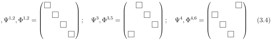
accord-ing to (2.2) gives aZZ4 orbifold theory, which restricts the form of the fields to be as follows:
Aµ,Ψ1,2,Φ1,2 =
; Ψ3,Φ3,5 =
; Ψ4,Φ4,6 =
(3.4)
where are 2×2 blocks. We recall from the previous section that we have chosen the R-symmetry
decomposition as4=12trivial⊕2 and 6=12trivial⊕22. The fields in (3.4) are defined in accordance thereto: the fermions Ψ1,2 and scalars Φ1,2 are respectively in the two trivial 1’s of the 4 and 6;
(Ψ3,Ψ4), (Φ3,Φ4) and (Φ5,Φ6) are in the doublet2of Γ inherited fromSU(2). Indeed, theRreg
ZZ4 (β4)
projection would force to be numbers and not matrices as we do not have the extra 112 tensored
to the group action, in which case (3.4) would be 4×4 matrices prescribing the adjacency matrices
[image:10.612.80.555.259.334.2]of the ZZ4 quiver. For this reason, the quiver diagram for the ZZ4 theory as drawn in part (I) of
Figure 1 has the nodes labelled 2’s instead of the usual Dynkin labels of 1’s for the A-series. In
physical terms we have placed twice as many image D-brane probes. The key point is that because
are now matrices (and (3.4) are 8×8), further projection internal thereto may change the number
and structure of the product gauge groups and matter fields.
Having done the first step by theβ4 projection, next we project with the regular representation
of γ:
RregD2(γ) =
1 0 0 −1
0 0 0
0 0 0
i 0 0 i
0 0
1 0 0 −1
0 0 i 0 0 i 0 0 :=
σ3 0 0 0
0 0 0 i112
0 0 σ3 0
0 i112 0 0
. (3.5)
In accordance with (3.4), let the gauge field be
Aµ :=
a 0 0 0
0 b 0 0
0 0 c 0
0 0 0 d
e
4e
3f
4f
3h
3h
4g
3
g
4 2
c
2b
2
a
2
d
NS5
NS5 NS5
D4
a
b
d
c
NS5
ON0 ON0
11
a
a
22c
11c
22NS5 NS5
D4
b
2b
11
a
a
22c
11c
22e
11h
12e
12h
21f
12g
11
f
21
g
12
1
1
1
1
D
24
ZZ
(I)
(II)
[image:11.612.68.534.93.476.2](IV)
(III)
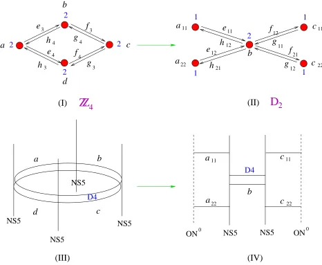
Figure 1: From the fact that D2 := hβ4, γi is generated by ZZ4 = β4 together with γ, our stepwise
projection, first by β4, and then byγ, gives 2 copies of the ZZ4 quiver in Part (I) and then the D2 quiver
in Part (II) by appropriate joining/splitting of the nodes and arrows. The brane configurations for these theories are given in Parts (III) and (IV).
with a, b, c, ddenoting the 2×2 blocks , (2.2) for (3.5) now reads
Aµ=Rreg D2(γ)
−1·Aµ·Rreg D2(γ)⇒
a 0 0 0
0 b 0 0
0 0 c 0
0 0 0 d
=
σ3 0 0 0
0 0 0 −i112
0 0 σ3 0
0 −i112 0 0
a 0 0 0
0 b 0 0
0 0 c 0
0 0 0 d
σ3 0 0 0
0 0 0 i112
0 0 σ3 0
0 i112 0 0
,
giving us a set of constraining equations for the blocks:
Similarly, for the fermions in the2, viz.,
Ψ3 =
0 e3 0 0
0 0 f3 0
0 0 0 g3
h3 0 0 0 , Ψ
4 =
0 0 0 e4
f4 0 0 0
0 g4 0 0
0 0 h4 0
,
the projection (2.2) is
γ· Ψ 3 Ψ4
=RregD 2(γ)
−1 · Ψ 3 Ψ4 ·RregD
2(γ).
We have used the fact that the induced action ρ(γ), having to act upon a doublet, is simply the
2×2 matrix γ herself. Therefore, writing it out explicitly, we have
i
0 0 0 e4
f4 0 0 0
0 g4 0 0
0 0 h4 0
=
σ3 0 0 0
0 0 0 −i112
0 0 σ3 0
0 −i112 0 0
0 e3 0 0
0 0 f3 0
0 0 0 g3
h3 0 0 0
σ3 0 0 0
0 0 0 i112
0 0 σ3 0
0 i112 0 0 and i
0 e3 0 0
0 0 f3 0
0 0 0 g3
h3 0 0 0
=
σ3 0 0 0
0 0 0 −i112
0 0 σ3 0
0 −i112 0 0
0 0 0 e4
f4 0 0 0
0 g4 0 0
0 0 h4 0
σ3 0 0 0
0 0 0 i112
0 0 σ3 0
0 i112 0 0 ,
which gives the constraints
f4 =−h3·σ3; g4 =σ3 ·g3; h4 =−f3·σ3; e4 =σ3·e3. (3.7)
The doublet scalars (Φ3,5,Φ4,6) of course give the same results, as should be expected from
super-symmetry.
In summary then, the final fields which survive both β4 and γ projections (and thus the entire
groupD2) are
Aµ=
a11 0
0 a22 !
b
c11 0
0 c22 ! b ;
e3=
e11 e12
0 0
!
, f3=
0 f12
0 f22 !
,
g3 =
g11 g12
0 0
!
, h3=
0 h12
0 h22 !
,
Ψ3=
0 e3 0 0
0 0 f3 0
0 0 0 g3
h3 0 0 0
, Ψ4=
0 0 0 σ3·e3
−h3·σ3 0 0 0
0 σ3·g3 0 0
0 0 −f3·σ3 0
2k ZZ
1
1
2 2 2
1
1
Dk
ON0 NS5
ON0 NS5
D4 D4
2
2
2 2
2
2
2
2
(II)
(III) (IV)
(I)
D4
NS5
NS5 NS5
NS5
NS5
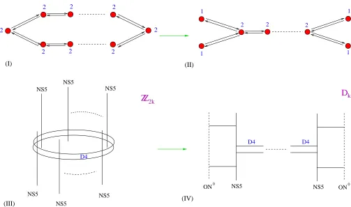
[image:13.612.51.554.87.384.2]NS5
Figure 2: Obtaining theDk quiver (II) from theZZ2k quiver (I) by the stepwise projection algorithm. The
brane setups are given respectively in (IV) and (III).
The key features to be noticed are now apparent in the structure of these matrices in (3.8). We
see that the 4 blocks of Aµ in (3.4), which give the four nodes of the
ZZ4 quiver, now undergo
a metamorphosis: we have written out the components of a, c explicitly and have used (3.6) to
restrict both to diagonal matrices, while b and d are identified, but still remain blocks without
internal structure of interest. Thus we have a total of 5 non-trivial constituentsa11, a22, c11, c22 and
b, precisely the 5 nodes of the D2 quiver (see parts (I) and (II) of Figure 1). Thus nodes of the
quiver merge and split as we impose further projections, as we mentioned a few paragraphs ago. As for the bifundamentals, i.e., the arrows of the quiver, (3.4) prescribes the blocks e3,4, f3,4, g3,4
andh3,4as the 8 arrows of Part (I) of Figure 1. After the projection byγ, and imposing the constraint
(3.7) as well as the fact that all entries of matter matrices must be non-negative, we are left with the 8 fields e11,12, f12,22, g11,12 and h12,22, precisely the 8 arrows in the D2 quiver (see Part (II) of
Figure 1).
The General Case
The generic situation of obtaining the Dk quiver from that of ZZ2k is completely analogous. We
would always have two end nodes of the ZZ2k quiver each splitting into two while the middle ones
3.2 The E6 Quiver from D2
We now move on to tackle the binary tetrahedral group E6 (with the relation that E6/D2 ∼=ZZ3),
whose generators are
β4 =
i 0
0 −i
!
, γ = 0 i
i 0
!
, δ := 1 2
1−i 1−i
−1−i 1 +i
!
.
We observe therefore that it has yet one more generator δ than D2, hence we need to continue our
stepwise projection from the previous subsection, with the exception that we should begin with more copies ofZZ4. To see this let us first present the irreducible matrix representations of the three
generators of E6:
β4 γ δ
Γ(1)1 1 1 1
Γ(1)2 1 1 ω3
Γ(1)3 1 1 ω2
3
Γ(2)4 β4 γ δ
Γ(2)5 β4 γ ω3δ
Γ(2)6 β4 γ ω32δ
Γ(3)7
−1 0 0
0 1 0
0 0 −1
0 0 −1
0 −1 0
−1 0 0
−i
2
i
√
2 −
i
2
−√1
2 0
1 √ 2
i
2 −
i
√ 2
i
2
The regular representation for these generators is therefore a matrix of size 3·12+ 3·22+ 33 = 24,
in accordance with (2.1).
Our first step is as with the case of D2, namely to change to a convenient basis wherein β4
becomes diagonal:
RregE6(β4) =RZZreg4 (β4)⊗116. (3.9)
The only difference between the above and (3.3) is that we have the tensor product with 116 instead
of 112, therefore at this stage we have a ZZ4 quiver with the nodes labeled 6 as opposed to 2 as in
Part (I) of Figure 1. In other words we have 6 times the usual number of D-brane probes. Under the basis of (3.9),
REreg6(γ) =
Σ3 0 0 0
0 0 0 i116
0 0 Σ3 0
0 i116 0 0
where Σ3 :=σ3⊗113 =
1 0 0 0 0 0 0 1 0 0 0 0 0 0 1 0 0 0 0 0 0 −1 0 0 0 0 0 0 −1 0 0 0 0 0 0 −1
. (3.10)
Subsequent projection gives a D2 quiver as in part (II) of Figure 1, but with the nodes labeled as
of regular representations ofD2 directly: RregE6(β4) =R
reg
D2(β4)⊗113 and R
reg
E6(γ) =R
reg
D2(γ)⊗113. To
this fact we shall later turn.
To arrive at E6, we proceed with one more projection, by the last generator δ, the regular
representation of which, observing the table above, has the form (in the basis of (3.9))
RregE6(δ) =
S1 0 S2 0
0 ω−81P 0 ω8−1P
S3 0 S4 0
0 −ω8P 0 ω
8P (3.11) where
S1 :=
1 0 0 0
!
⊗RregZZ3(β3), S2 :=
0 0 1 0 ! ⊗
0 0 1 0 1 0 1 0 0
,
S3 :=−i
0 0 0 1 ! ⊗
0 0 1 0 1 0 1 0 0
, S4 :=i
0 1 0 0
!
⊗113
and
P :=RregZZ3 (β3)⊗
1 √
2112; recalling that R reg
ZZ3(β3) :=
1 0 0
0 ω3 0
0 0 ω2
3 .
The inverse of (3.11) is readily determined to be
RregE6(δ)−1 =
˜
S1 0 −S3 0
0 1
2ω8P−
1 0 −1
2ω− 1 8 P−1
ST
2 0 −S4T 0
0 1
2ω8P−
1 0 1
2ω− 1 8 P−1
, ˜
S1 :=
1 0 0 0
!
⊗RregZZ3 (β3)−1.
Thus equipped, we must use (2.2) with (3.11) on the matrix forms obtained in (3.8) (other fields can of course be checked to have the same projection), with of course each number therein now being 3×3 matrices. The final matrix forAµ is as in (3.8), but with
a11=
a11(1) 0 0
0 a11(2) 0
0 0 a11(3)
3×3
; c11 =c22=a22; b =
b11 0 0
0 b22 0
0 0 b33
6×6
where a22, cii are 3×3 while bii are 2×2 blocks. We observe therefore, that there are 7 distinct gauge group factors of interest, namely a11(1), a11(2), a11(3), a22, b11, b22 and b33, with Dynkin labels
1,1,1,3,2,2,2 respectively. What we have now is the E6 quiver and the bifundamentals split and
3.3 The E6 Quiver from ZZ6
Let us make use of an interesting fact, that actually E6 = hβ4, γ, δi = hβ4, δi = hγ, δi. Therefore,
alternative to the previous subsection wherein we exploited the sequenceZZ4 =hβ4i +γ
−→D2 −→+δ E6,
we could equivalently apply our stepwise projection onZZ6 =hδi +β4
−→E6.
Let us first project with δ, an element of order 6 and the regular representation of which, after appropriate rotation is
RregE6(δ) =RZZreg6 (δ)⊗114. (3.12)
Therefore at this stage we have aZZ6 quiver with labels of six 4’s due to the 114; this is drawn in Part
(II) of Figure 3. The gauge group we shall denote asAµ := Diag(a, b, c, d, e, f)
24×24, with a, b,· · ·, f
being 4×4 blocks.
Next we perform projection by RregE6(β4) in the rotated basis, splitting and joining the gauge
groups (nodes) as follows
Aµ =
a 11 0 0 ˜a
0 0 0 0 0
0 b
1 0 0 b2
0 0 0 0
0 0
c 11 0 0 ˜c
0 0 0
0 0 0
d 1 0 0 d2
0 0
0 0 0 0
e 11 0 0 ˜e
0
0 0 0 0 0
f 1 0 0 f2
; s. t.
˜
a= ˜c= ˜e, b2 =d1,
d2 =f1,
f2 =b1,
which upon substitution of the relations, gives us 7 independent factors: a11, c11ande11are numbers,
giving 1 as Dynkin labels in the quiver;b1, b2 and d2 are 2×2 blocks, giving the 2 labels; while ˜a is
3×3, giving the 3. We refer the reader to Part (II) of Figure 3 for the diagrammatical representation.
4. Comments and Discussions
Our procedure outlined above is originally inspired by a series of papers [10, 11, 12], where the quivers for the ∆ series of Γ⊂SU(3) were observed to be obtainable from theZZn×ZZn series after an appropriate identification. In particular, it was noted that
∆(3n2) = h
ZZn×ZZn :=
ωi
n 0 0
0 ωjn 0 0 0 ω−i−j
n !
i,j=0,···,n−1
,
0 0 1 1 0 0 0 1 0
!
,
0 1 0 0 0 1 1 0 0
!
i and subsequently
the quiver for ∆(3n2) is that of
ZZn×ZZn modded out by a certain ZZ3 quotient. Similarly, the quiver
for
∆(6n2) = hZZn×ZZn,
0 0 1 1 0 0 0 1 0
!
,
0 1 0 0 0 1 1 0 0
!
, −
1 0 0 0 0 −1 0 −1 0
!
,
0 −1 0 −1 0 0 0 0 −1
!
,
0 0 −1 0 −1 0 −1 0 0
!
i
is that ofZZn×ZZn modded out by a certainS3 quotient. In [12], it was further commented that the
11
a
a22
c11
c22
e11 h12
e12
h21
f12 g11
f21 g
12
3
3
3
6
b
3
4
4 4
4
4 a b
f c
d
e 4
e4 e3
f4 f3
h3
h4
g3 g
4 6
c 6
b
6 a
6 d
11(1)
a
a11(2)
a11(3)
22
b
33
b
11
b
c11 c22
a22 = =
~
a ~c
~ e = =
11
a
c11
e11
2
b = d1 1
b = f2
2
d = f1
1
1
1
2 3
2
2
6
ZZ
4
ZZ
D
2E
6(I) 1
1
1
3 2
2 2
[image:17.612.69.534.98.495.2](II)
Figure 3: Obtaining the quiver diagram for the binary tetrahedral group E6. We compare the two
alternative stepwise projections: (I) ZZ4 = hβ4i → D2 = hβ4, γi → E6 = hβ4, γ, δi and (II) ZZ6 = hδi →
E6=hδ, β4i.
The motivation for those studies was to realise a brane-setup for the non-AbelianSU(3) orbifolds
as geometrical quotients of the well-known Abelian case of ZZm×ZZn, viz., the Brane Box Models.
The key idea was to recognise that the irreducible representations of these groups could be labelled by a double index (l1, l2)∈ZZn×ZZn up to identifications.
4.1 A Mathematical Viewpoint
To see why our stepwise projection works on a more axiomatic level, we need to turn to a brief review of the Theory of Induced Representations.
It was a fundamental observation of Frøbenius that the representations of a group could be constructed from an arbitrary subgroup. The aforementioned chain of groups, where we tried to relate the regular representations, is precisely in this vein. Though we shall largely follow the nomenclature of [13], we shall now briefly review this theory in the spirit of the above discussions. Let Γ1 = hx1, ..., xni and Γ2 = hx1, ..., xn+1i. We see thus that Γ1 ⊂ Γ2. Now let RΓ1(x) be a
representation (not necessarily irreducible) of the element x∈Γ1. Extending it to Γ2 gives
RΓ2(y) =
RΓ1(x) if y=x∈Γ1
0 if y6∈Γ1
It follows then that if we decompose Γ2 as (right) cosets of Γ1,
Γ2 = Γ1t1∪Γ1t2∪ · · · ∪Γ1tm
we have anInduced Representation of Γ2 as
RΓ2(y) = RΓ1(tiyt− 1
j ) =
RΓ1(t1yt− 1
1 ) RΓ1(t1yt− 1
2 ) · · · RΓ1(t1yt− 1
m )
RΓ1(t2yt− 1
1 ) RΓ1(t2yt− 1
2 ) · · · RΓ1(t2yt− 1
m )
... ... ...
RΓ1(tmyt− 1
1 ) RΓ1(tmyt− 1
2 ) · · · RΓ1(tmyt− 1
m )
. (4.1)
A beautiful property of (4.1) is that it has only one member of each row or column non-zero and whereby it is essentially a generalised permutation (see e.g., 3.1 of [13]) matrix acting on the Γ1-stable submodules of the Γ2-module.
Now, for the case at hand the coset decomposition is simple due to the addition of a single new generator: the (right) transversals t1,· · ·, tm are simply powers of the extra generator xn+1 and m
is simply the index of Γ1 ⊂Γ2, namely |Γ2|/|Γ1|, i.e.,
ti =xin−+11 i= 1,2,· · ·, m; m= |
Γ2|
|Γ1|
. (4.2)
Now let us define an important concept for an element x∈ Γ2
DEFINITION 4.1 We call a representation RΓ2(x) factorisable if it can be written, up to possible
change of bases, as a tensor product RΓ2(x) =RΓ1(x)⊗11k for some integer k.
could continue with the stepwise algorithm to demonstrate how the nodes of these copies merge or
split. In the corresponding D-brane picture this simply means that we should consider k copies of
each image D-brane probe in the covering space.
The natural question to ask is of course why our examples in the previous section permitted factorisable generators so as to in turn permit the performance of the stepwise projection. The following claim shall be of great assurance to us:
PROPOSITION 4.1 Let H be a subgroup of G, then the representation RG(x) for an element x ∈ H ⊂ G induced from RH(x) according to (4.1) is factorisable and k is equal to |G|/|H|, the index of H in G.
Proof: Take RH(x ∈ H), and tensor it with 11k=|G|/|H|; this remains of course a representation
for x ∈ H. It then remains to find the representations of x 6∈ H, which we supplement by the
permutation actions of these elements on the H-cosets. At the end of the day we arrive at a
representationR′
G(x) of dimensionk, such that it is factorisable forx∈Hand a general permutation
for x 6∈ H. However by the uniqueness theorem of induced representations (q.v. e.g. [14] Thm
11) such a linear representation R′
G(x) must in fact be isomorphic to RG(x). Thus by explicit
construction we have shown that RG(x∈H) =RH(x)⊗11k.
We can be more specific and apply Proposition 4.1 to our case of the two groups the second of which is generated by the first with one additional generator. Using the elegant property that the induction of a regular representation remains regular (q.v. e.g., 3.3 of [14]), we have:
COROLLARY 4.1 Let Γ1 and Γ2 be as defined above, then
RregΓ2 (xi) =RregΓ1 (xi)⊗11|Γ2|/|Γ1| for common generators i= 1,2, . . . , n.
In particular, since any G = hx1, . . . , xni contains a cyclic subgroup generated by, say x1 of order
m, i.e., ZZm =hx1i, we conclude that
COROLLARY 4.2 RregG (x1) = RregZZm(x1)⊗11|G|/m, and hence the quiver for G can always be obtained
by starting with the ZZm quiver using the stepwise projection.
Let us revisit the examples in the previous section equipped with the above knowledge. For the case of Γ1 = ZZ4 =hβ4i and Γ2 = D2 with the extra generator γ, (4.2) becomes t1 = 11 and t2 = γ
as the index of ZZ4 inD2 is ||DZZ42||=4=8 = 2. The induced representation ofβ4 according to (4.1) reads
RD2(β4) =
Rreg
ZZ4 (11β411
−1) Rreg
ZZ4 (11β4γ −1)
Rreg
ZZ4 (γβ411
−1) Rreg
ZZ4 (γβ4γ −1)
!
= R
reg
ZZ4 (β4) 0
0 Rreg
ZZ4 (β −1 4 )
!
using the fact thatγβkγ−1 =βk−1 inDk for the last entry. Recalling that RregZZ4(β4) =
1 0 0 0 0 i 0 0 0 0 i2 0 0 0 0 i3
,
this is subsequently equal to Rreg
manifests her validity as we see that the RD2 obtained by Frøbenius induction of R
reg
ZZ4 is indeed
regular and moreover factorisable, as (3.3) dictates.
Similarly with the case of ZZ6 → E6, we see that Corollary 4.1 demands that for the common
generator δ, REreg6(δ) should be factorisable, as is indeed indicated by (3.12). So too is it with
ZZ4 →E6, where RregE6(β4) should factorise, precisely as shown by (3.9).
The above have actually been special cases of Corollary 4.2, where we started with a cyclic subgroup; in fact we have also presented an example demonstrating the general truism of Proposition 4.1. In the case of D2 → E6, we mentioned earlier that REreg6(β4) = R
reg
D2(β4)⊗113 and R
reg E6(γ) =
RregD2(γ)⊗113for the common generators as was seen from (3.9) and (3.10); this is exactly as expected
by the Proposition.
4.2 A Physical Viewpoint: Brane Setups?
Now mathematically it is clear what is happening to the quiver as we apply stepwise projection. However this is only half of the story; as we mentioned in the introduction, we expect T-duality to take D-branes at generic orbifold singularities to brane setups. It is a well-known fact that the brane setups for theA andD-type orbifolds C2/ZZn and C2/Dnhave been realised (see [15, 16] and [19] respectively). It has been the main intent of a collective of works (e.g [9, 11, 12]) to establish such setups for the generic singularity.
In particular, the problem of finding a consistent brane-setup for the remaining case of the exceptional groupsE6,7,8 of the ADE orbifold singularities of C2 (and indeed analogues thereof for
SU(3) and SU(4) subgroups) so far has been proven to be stubbornly intractable. An original
motivation for the present work is to attempt to formulate an algorithmic outlook wherein such a problem, with the insight of the algebraic structure of an appropriate chain of certain relevant groups, may be addressed systematically.
4.2.1 The ZZ2 Action on the Brane Setup
Let us attempt to recast our discussion in Subsection 3.1 into a physical language. First we try to interpret the action by RregDk(γ) in (3.2) on the ZZ2k quiver as a string-theoretic action on brane setups to get the corresponding brane setup of Dk from that ofZZ2k.
Now the brane configuration for the ZZ2k orbifold is the well-known elliptic model consisting
of 2k NS5-branes arranged in a circle with D4-branes stretched in between as shown in Part (III)
of Figure 1. After stepwise projection by γ, the quiver in Part (I) becomes that in Part(II) (see
Figure 2 also). There is an obvious ZZ2 quotienting involved, where the nodes i and 2k − i for
i= 1,2, ..., k−1 are identified while each of the nodes 0 andk splits into two parts. Of course, this
symmetry is not immediately apparent from the properties ofγ, which is a group element of order
Let us digress a moment to formulate the above results in the language used in [10, 11]. Recalling from the brief comments in the beginning of Section 4, we adopt their idea of labelling the irreducible representations of ∆ byZZn×ZZnup to appropriate identifications, which in our terminology is simply
the by-now familiar stepwise projection of the parent ZZn×ZZn quiver. As a comparison, we apply
this idea to the case ofZZ2k→Dk. Therefore we need to label the irreps of Dk or appropriate tensor
sums thereof, in terms of certain (reducible) 2-dimensional representations of ZZ2k. Motivated by
the factorization property (3.3), we chose these representations to be
RlZZ2k(2) :=Rl,irrepZZ2k(1) ⊕Rl,irrepZZ2k(1) (4.3) wherel∈ZZ2k, and amounts to precisely aZZ2k-valued index on the representations ofDk (sinceZZ2k is Abelian), which with foresight, we shall later use onDk. We observe that such a labelling scheme has a symmetry
RlZZ2k(2) ∼=RZZ−2lk(2),
which is obviously a ZZ2 action. Note that l = 0 and l =k are fixed points of this ZZ2.
We can now associate the 2-dimensional irreps of Dk with the non-trivial equivalence classes of
the ZZ2k representations (4.3), i.e., forl = 1,2, . . . , k−1 we have
RlZZ2k(2) ∼=R−ZZ2lk(2) →R
l,irrep
Dk(2). (4.4)
These identifications correspond to the merging nodes in the associated quiver diagram. As for the fixed points, we need to map
R0
ZZ2k(2) →R 1,irrep Dk(1) ⊕R
2,irrep Dk(1)
Rk
ZZ2k(2) →R 3,irrep Dk(1) ⊕R
4,irrep Dk(1) .
(4.5)
These fixed points are associated precisely with the nodes that split.
This construction shows clearly how, in the labelling scheme of [10, 11], our stepwise algorithm derives the Dk quiver as a ZZ2 projection of the ZZ2k quiver. The consistency of this description is verified by substituting the representations Rl
ZZ2k(2) in the ZZ2k quiver relations R ⊗ R
l
ZZ2k(2) = L
¯
l
aZZ2k(R)
l¯l R
¯
l
ZZ2k(2) using (4.4) and (4.5), which results exactly in the Dk quiver relations. We can of
course apply the stepwise projection for the case ofZZn×ZZn →∆, and would arrive at the results in [10, 11].
In the brane setup picture, the identification of the nodes i and 2k −i for i = 1,2, ..., k−1 corresponds to the identification of these intervals of NS5-branes as well as the D4-branes in between
in the X6789 directions (with direction-6 compact). Thus the
ZZ2 action on the ZZ2k quiver should include a space-time action which identifiesX6789 =−X6789. Similarly, the splitting of gauge fields
in intervals 0 and k hints the existence of a ZZ2 action on the string world-sheet. Thus the overall
ZZ2 action should include two parts: a space-time symmetry which identifies and a world-sheet
What then is this action physically? What object in string theory performs the tasks in the above paragraph? Fortunately, the space-time parity and string world-sheet (−1)FL actions [18, 19]
are precisely the aforementioned symmetries. In other words, the ON-plane is that which we seek.
This is of great assurance to us, because the brane setup forDk theories, as given in [19], is indeed a configuration which uses the ON-plane to project out or identify fields in a manner consistent with our discussions.
4.2.2 The General Action on the Brane Setup?
It seems therefore, that we could now be boosted with much confidence: since we have proven in the previous subsection that our stepwise projection algorithm is a constructive method of arriving
at any orbifold quiver by appropriate quotient of the ZZn quiver, could we not simply find the
appropriate object in string theory which would perform such a quotient, much in the spirit of the orientifold prescribingZZ2 in the above example, on the well-knownZZn brane setup, in order to solve our problem?
Such a confidence, as is with most in life, is overly optimistic. Let us pause a moment to consider theE6 example. The action byδin the case ofD2 →E6in§3.2 and that ofβ4 in the case ofZZ6 →E6
in§3.3 can be visualised in Parts (I) and (II) of Figure 3 to be anZZ3 action on the respective parent
quivers. In particular, the identifications c11 ∼ c22 ∼ a22 and ˜a ∼ c˜∼ e˜;b1 ∼ f2, b2 ∼ d1, d2 ∼ f1
respectively for Parts (I) and (II) are suggestive of a ZZ3 action on X6789. The tripartite splittings
forb, a11 and a, b, d respectively also hint at aZZ3 action on the string world-sheet.
Again let us phrase the above results in the scheme of [10, 11], and manifestly show how the
E6 quiver results from a ZZ3 projection of the D2 quiver. We define the following representations of
D2: R0D2(6) =R
irrep D2(2)⊕R
irrep D2(2)⊕R
irrep
D2(2) and R
l
D2(3) =R
l,irrep D2(1) ⊕R
l,irrep D2(1) ⊕R
l,irrep
D2(1) where l ∈ZZ4 labels
the four 1-dimensional irreducible representations ofD2. There is an identification
Rl D2 ∼=R
f(l)
D2
where
f(l) =
0, l= 0 2, l= 1 3, l= 2 1, l= 3
Clearly this is aZZ3 action on the index l. Note that we have two representations labelled with l= 0
which are fixed points of this action. In the quiver diagram of D2 these correspond to the middle
E6 quiver we need to map the nodes of the parent D2 quiver as
R0
D2(6) →R 1,irrep E6(2) ⊕R
2,irrep E6(2) ⊕R
3,irrep E6(2)
R0
D2(3) →R 1,irrep E6(1) ⊕R
2,irrep E6(1) ⊕R
3,irrep E6(1)
Rl
D2(3) ∼=R
f(l)
D2(3) →R
irrep
E6(3), l∈ZZ4− {0}.
Consistency requires that if we replace RD2 in the D2 quiver defining relations and then use the
above mappings, we get the E6 quiver relations forRirrepE6 .
The origin of this ZZ3 analogue of the orientifold ZZ2-projection is thus far unknown to us. If an
object with this property is to exist, then the brane setup for theE6 theory could be implemented;
on the other hand if it does not, then we would be suggested at why the attempt for E6 has been
prohibitively difficult.
The ZZ3 action has been noted to arise in [11] in the context of quotienting the ZZn×ZZn quiver to arrive at the quiver for the ∆-series. Indeed from our comparative study in Section 4.2.1, we see that in general, labelling the irreps by a multi-index is precisely our stepwise algorithm in disguise, as applied to a product Abelian group: the ZZn× · · · ×ZZn orbifold. Therefore in a sense we have explained why the labelling scheme of [10, 11] should work.
And the same goes with E7 and E8: we could perform stepwise projection thereupon and
mathematically obtain their quivers as appropriate quotients of the ZZn quiver by the symmetry S
of the identification and splitting of nodes. To find a physical brane setup, we would then need to
find an object in string theory which has anS action on space-time and the string world-sheet. Note
that the above are cases of the C2 orbifolds; for the Ck-orbifold we should initialise our algorithm with, and perform stepwise projection on the quiver ofZZn× · · · ×ZZn (k−1 times), i.e., the brane box and cube (k= 2,3).
Though mathematically we have found a systematic treatment of constructing quivers under a new light, namely the “stepwise projection” from the Abelian quiver, much work remains. In the field of brane setups for singularities, our algorithm is intended to be a small step for an old standing
problem. We must now diligently seek a generalisation of the orientifold plane with symmetry S in
string theory, that could perform the physical task which our mathematical methodology demands.
Acknowledgements
Ad Catharinae Sanctae Alexandriae et Ad Majorem Dei Gloriam...
We would like to extend our gratitude to D. Berenstein for useful discussions, especially for his informing us of his related works in the context of discrete torsion. Furthermore, we are indebted to the Reed Fund, the CTP, and the LNS for their gracious patronage.
References
[2] Clifford V. Johnson, Robert C. Myers, “Aspects of Type IIB Theory on ALE Spaces,” hep-th/9610140.
[3] A. Hanany and E. Witten, “Type IIB Superstrings, BPS monopoles, and Three-Dimensional Gauge Dynamics,” hep-th/9611230.
[4] A. Giveon and D. Kutasov, “Brane Dynamics and Gauge Theory,” hep-th/9802067.
[5] A. Lawrence, N. Nekrasov and C. Vafa, “On Conformal Field Theories in Four Dimensions,” hep-th/9803015.
[6] E. Rabinovici, Talk, Strings 2000.
[7] A. Hanany and Y.-H. He, “Non-Abelian Finite Gauge Theories,” hep-th/9811183.
[8] A. Hanany and Y.-H. He, “A Monograph on the Classification of the Discrete Subgroups ofSU(4),” hep-th/9905212.
[9] B. Feng, A. Hanany, and Y.-H. He, “TheZk×Dk′ Brane Box Model,” hep-th/9906031;
B. Feng, A. Hanany, and Y.-H. He, “Z-D Brane Box Models and Non-Chiral Dihedral Quivers,” hep-th/9909125.
[10] T. Muto, “D-branes on Three-dimensional Nonabelian Orbifolds,” hep-th/9811258.
[11] T. Muto, “Brane Configurations for Three-dimensional Nonabelian Orbifolds,” hep-th/9905230.
[12] T. Muto, “Brane Cube Realization of Three-dimensional Nonabelian Orbifolds,” hep-th/9912273.
[13] W. Ledermann, “Introduction to Group Characters,” CUP, Cambridge 1987.
[14] J.-P. Serre, “Linear Representations of Finite Groups,” Springer-Verlag, 1977.
[15] A. Hanany and A. Zaffaroni, “On the Realisation of Chiral Four-Dimensional Gauge Theories Using Branes,” hep-th/9801134.
[16] A. Hanany and A. Uranga, “Brane Boxes and Branes on Singularities,” hep-th/9805139.
[17] H. Garc´ıa-Compe´an and A. Uranga, “Brane Box Realization of Chiral Gauge Theories in Two Di-mensions,” hep-th/9806177.
[18] A. Sen, “Duality and Orbifolds,” hep-th/9604070;
A. Sen, “Stable Non-BPS Bound States of BPS D-branes”, hep-th/9805019.
[19] A. Kapustin, “Dn Quivers from Branes,” hep-th/9806238.
[20] A. Uranga, “From quiver diagrams to particle physics,” hep-th/0007173.
[21] D. Berenstein, Private communications;