A conceptual framework and taxonomy of techniques for analyzing movement

City, University of London Institutional Repository

Citation

:

10.1016/j.jvlc.2011.02.003

This is the unspecified version of the paper.

This version of the publication may differ from the final published

version.

Permanent repository link:

Link to published version

:

Copyright and reuse:

City Research Online aims to make research

outputs of City, University of London available to a wider audience.

Copyright and Moral Rights remain with the author(s) and/or copyright

holders. URLs from City Research Online may be freely distributed and

linked to.

City Research Online: http://openaccess.city.ac.uk/ [email protected]

A Conceptual Framework and Taxonomy of Techniques for

Analyzing Movement

G. Andrienko1, N. Andrienko1, P. Bak2, D. Keim3, S. Kisilevich3, S. Wrobel1 1_{Fraunhofer Institute IAIS - Intelligent Analysis and Information Systems}

Schloss Birlinghoven, Sankt-Augustin, D-53754 Germany 2

IBM Haifa Research Lab, Mount Carmel, IL-31905, Israel 3

A Conceptual Framework and Taxonomy of Techniques for

Analyzing Movement

Abstract

Movement data link together space, time, and objects positioned in space and time. They hold valuable and multifaceted information about moving objects, properties of space and time as well as events and processes occurring in space and time. We present a conceptual framework that describes in a systematic and comprehensive way the possible types of information that can be extracted from movement data and on this basis defines the respective types of analytical tasks. Tasks are distinguished according to the type of information they target and according to the level of analysis, which may be elementary (i.e. addressing specific elements of a set) or synoptic (i.e. addressing a set or subsets). We also present a taxonomy of generic analytic techniques, in which the types of tasks are linked to the corresponding classes of techniques that can support fulfilling them. We include techniques from several research fields: visualization and visual analytics, geographic information science, database technology, and data mining.

A Conceptual Framework and Taxonomy of Techniques for

Analyzing Movement

1 Introduction

Spatio-temporal data, in particular, movement data, involve geographical space, time, various objects existing and occurring in space, and multidimensional attributes changing over time. This complexity poses significant challenges for the analysis; however, it also enables the use of the data for many purposes: to study the properties of space and places, to understand the temporal dynamics of events and processes, to investigate behaviours of moving objects, and so on. Hence, there is a great variety of possible analysis tasks related to spatio-temporal data. In many applications, spatio-temporal data are generated in rapidly growing amounts. In response, a large number of methods and tools for dealing with these data have been developed in several research fields: visualization and visual analytics, geographic

information science, database technology, and knowledge discovery in databases (also known as data mining). Currently, there is no systematic classification of the existing approaches to analyzing spatio-temporal data. This is a disadvantage both for data analysts and for

researchers devising new analytical methods. Analysts have difficulties with finding suitable methods for their data and tasks, especially taking into account that methods are developed in several disciplines. Moreover, methods created in different disciplines are often

complementary and should be used in combination. Researchers may know well the state of the art in their own area but be insufficiently aware about the efforts made in the other disciplines and therefore miss potentially useful ideas and approaches from these disciplines. Our research addresses this problem. We do not attempt to produce a complete inventory of all specific techniques, algorithms, and software tools created in different research areas. It is not only hard but also not really useful since such a survey would soon become outdated. Instead, we suggest a taxonomy of generic approaches to analyzing spatio-temporal data, in particular, data related to movement. Generic approaches correspond to groups of methods. For example, spatial clustering of points is a generic approach corresponding to a large group of specific clustering algorithms.

Our taxonomy is based on a conceptual framework defining the possible types of spatio-temporal data and possible types of analysis tasks. The generic approaches are linked to the types of data and tasks they are suitable for. Therefore, the taxonomy may be useful both for data analysts and for researchers developing new methods. Data analysts will be able to find generic approaches suitable for their data and tasks and then refer to the respective fields for specific methods and/or tools. Researchers will be able to learn what generic approaches exist in different fields for the types of data and tasks they are going to deal with and compare or relate these approaches to their own ideas. The researchers will also be able to position their new methods in the taxonomy.

The paper is structured as follows. In Section 2 we briefly review the research related to defining types of data and analysis tasks. In Section 3 we present our conceptual framework and in Section 4 describe on this basis the structures of data related to movement. Section 5 deals with the possible transformations of movement data. Section 6 presents the taxonomy of the generic analytic techniques. Before concluding, we give in Section 7 examples of several methods applied to a real world dataset. The data and respective analysis tasks are

2 Related

research

Our conceptual framework aims at describing the possible types of information that can be extracted from movement data and defining the respective types of analytical tasks. Hence, the related research includes the works where possible types of analysis tasks, or questions, are defined according to the components of data, particularly spatio-temporal data.

Peuquet (1994, 2002) distinguishes three components in spatio-temporal data: space (where), time (when), and objects (what). Accordingly, Peuquet defines three basic kinds of questions: ƒ when + where → what: Describe the objects or set of objects that are present at a given

location or set of locations at a given time or set of times.

ƒ when + what → where: Describe the location or set of locations occupied by a given object or set of objects at a given time or set of times.

ƒ where + what → when: Describe the times or set of times that a given object or set of objects occupied a given location or set of locations.

Blok (2000) and Andrienko et al. (2003) define analysis tasks for spatio-temporal data based on the types of changes occurring over time:

1. Existential changes, i.e. appearance and disappearance.

2. Changes of spatial properties: location, shape or/and size, orientation, altitude, height, gradient, and volume.

3. Changes of thematic properties expressed through values of attributes: qualitative changes and changes of ordinal or numeric characteristics (increase and decrease).

Bertin (1983) introduces the notions of “question types” and “reading levels”. The notion of question types refers to components (variables) present in data: “There are as many types of questions as components in the information” (Bertin 1983, p.10). For each question type, there are three reading levels, elementary, intermediate, and overall. The reading level indicates whether a question refers to a single data element, to a group of elements, or to the whole phenomenon characterized by all elements. Andrienko et al. (2003) argue that there is no fundamental difference between the intermediate and overall levels and suggest joining these into a single notion. Andrienko and Andrienko (2006) distinguish elementary and synoptic analysis tasks.

Our conceptual framework for analysis of movement data builds on these approaches and elaborates the concepts presented by Andrienko et al. (2008).

3 Conceptual

framework

3.1 Fundamental sets: space, time, and objects

The set of objects includes various physical and abstract entities. Objects can be classified according to their spatial and temporal properties. A spatial object is an object having a particular position in space in any time moment of its existence. Temporal object, also called

event, is as an object with limited time of existence with respect to the time period under observation, or, in other words, an object having a particular position in time. Spatial events

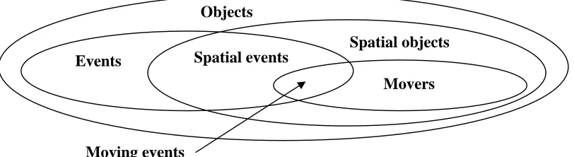
are objects having particular positions in space and time. Moving object, also called mover, is a kind of spatial object capable to change its spatial position over time. Moving events are events that change their spatial positions over time (e.g. hurricane, parade). Spatial events and movers can be jointly called spatio-temporal objects. The Venn diagram in Figure 1 illustrates the is-a relations between the types of objects. From now on, we consider only objects having positions in time and/or in space, i.e. events and spatial objects.

Figure 1. The is-a relations between the types of objects.

Movement is the change of the spatial position(s) of one or more movers over time. Changes of the spatial position of one mover be represented by a mapping (function) τ: T→S, which is called trajectory. Movement of multiple objects can be represented as a function μ: O×T→S. A trajectory consists of pairs (t,s), t∈T, s∈S. Each pair has a particular position s in space and a particular position t in time; in our classification, it is a spatial event. Hence, a trajectory consists of spatial events. Furthermore, a trajectory itself is a spatial object whose position in space is the set of places visited by the mover. When the mover is treated as a point (i.e., the shape and size are ignored), the spatial position of the trajectory is a line in S. A trajectory has also a certain position in time, which is the time interval when the positions of the mover were observed. This interval does not necessarily coincide with the whole time of the mover’s existence. According to our definition, a trajectory is a spatial event. This is a complex spatial event consisting of a sequence of elementary spatial events (t,s). Hence, spatial events are intrinsic in movement.

3.2 Spatio-temporal context

In the formal model of movement, time and space are mathematical abstractions. In reality, analysts have to deal with physical (most often geographical) space and physical time. The main difference of physical space and physical time from their mathematical abstractions is heterogeneity, i.e. variation of properties from position to position. In geographical space, water differs from land, mountain range from valley, forest from meadow, seashore from inland, city centre from suburbs, and so on. It can be said that every location has some degree of uniqueness relative to the other locations. The same applies to other physical spaces such as inner spaces of buildings or the space of human body. In physical time, day differs from night, winter from summer, working days from weekends, etc. In considering relations of objects to space or time, the analyst is usually not so much interested in abstract spatial or

Objects

Events

Spatial objects Spatial events

Movers

temporal positions as in the respective physical locations or times with their properties. For example, wild animals may have their preferred types of locations such as forest or meadow, may move differently in forest-covered and open places, may move actively in certain times of a day and stay still in other times, may migrate seasonally, and so on.

Heterogeneous properties of locations and times constitute a part of the context in which spatial and temporal objects exist and move. Another part of the context, with regard to each object, consists of the other objects that exist in the same space and time.

3.3 Characteristics of objects, locations, and times

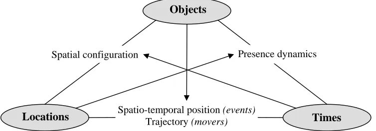
Here we consider how elements of each of the basic three sets can be characterized in terms of the other two sets. As already mentioned, events are characterized by their spatio-temporal positions and movers by their trajectories. Presence dynamics is a dynamic (time-dependent) attribute characterizing a location in terms of the objects that are present in it. This can be represented by a function T→P(O), where P(O) is the power set (i.e. the set of all subsets) of O. Spatial configuration is an attribute characterizing a time unit in terms of the objects existing in this time unit and their spatial positions. This can be represented by a function O→S. Figure 2 summarizes the characteristics in a graphical form. This scheme has a clear relation to the triad model “what, when, where” by D.Peuquet (1994).

Figure 2. Characteristics of objects, locations, and times.

As mentioned before, objects, locations, and times may have thematic attributes. Thematic attributes of objects and locations may be static (i.e. values do not change over time) or dynamic, for example, attributes of movers reflecting the speed and direction of the movement. A dynamic attribute may be represented by a mapping from T to some domain (set) D containing possible values of the attribute. Some dynamic thematic attributes may be derived from trajectories (for movers) and from presence dynamics (for locations).

Trajectories may be used to compute speeds, directions, and other attributes of the movement. Presence dynamics may be used to derive counts of the objects, statistics of their thematic attributes (average, minimum, maximum, mode, etc.), and statistics of the times spent by the objects in the locations.

A time unit can be characterized not only in terms of spatial positions of objects but also in terms of their dynamic thematic attributes. All together can be represented by a function O→S×D1×…×Dn, where D1, …, Dn are the domains of time-dependent thematic attributes. We shall call it object configuration; note that it includes the spatial configuration O→S. Since locations may have their dynamic attributes not related to presence of objects, time units may be additionally characterized by the values of these attributes attained in different

Objects

Locations Spatio-temporal position _{Trajectory (movers)}(events) Times

locations in these time units (called spatial distribution of attribute values). This may be represented by a mapping S→D1×…×Dn, where D1, …, Dn are the domains of the dynamic attributes of the locations. Time units may also have various thematic attributes not related to places or objects. We shall use the term situation to denote the composition of object

configuration, spatial distribution of attribute values, and values of time-specific thematic attributes in a given time unit.

3.4 Relations

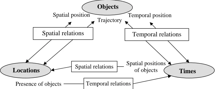
Here we consider what relations may exist among elements between the sets and within the sets. We focus on those types of relations that involve objects and space or time (or both space and time). Figure 3 shows how objects are related to locations and times and how locations and times are related in terms of objects. The spatial positions of objects are linked to locations by spatial relations. The temporal positions of objects are linked to times by temporal relations. Trajectories of movers, which include both space and time, are linked to locations by spatial relations and to times by temporal relations.

Locations by themselves do not have positions in time and, hence, relations to times. Locations may be related to times by the temporal objects (events and movers) appearing in the locations: the temporal positions of objects’ presence in the locations are linked to times by temporal relations. Likewise, times by themselves have no relations to locations but the spatial positions of objects in each time unit are linked to locations by spatial relations.

Figure 3. Relations between the sets of objects, locations, and times.

The types of spatial and temporal relations are considered in the literature on temporal and spatial reasoning (e.g. Allen 1983, Egenhofer 1991) and on geographic information systems (e.g. Jones 1997). The basic types of relations include binary topological, directional, and distance relations. For time units, directional relations are also known as ordering relations. On the basis of these primitives, more complex types of relations can be defined such as density (clustering, dispersion) and regularity.

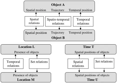
Figure 4 summarizes the relations among elements within the sets that involve elements of the other sets. The scheme shows that there are spatial relations among objects based on their spatial positions and temporal relations based on the temporal positions. Spatio-temporal relations occur among spatio-temporal objects, which include spatial events and movers. Spatio-temporal relations among objects that do not change their spatial positions are compositions of spatial and temporal relations. These include, in particular, spatio-temporal clustering or dispersion. Movers change their spatial positions and, hence, their relations to

Objects

Locations _Times

Spatial position Temporal position

Trajectory

Spatial relations _{Temporal relations}

Temporal relations Spatial relations

Presence of objects

places and to other objects. Spatio-temporal relations represent changes of spatial relations over time: approaching or going away, entering or exiting, following, keeping distance, concentrating or dissipating, etc. (Dodge et al. 2008).

Figure 4. Relations between objects, between locations, and between times.

Locations are linked by set relations (e.g. inclusion, overlap, etc.) based on the sets of the objects existing in these locations or visiting them and by temporal relations based on the temporal positions of the events occurring in these locations (including visits of these places by movers). The set relations change over time. Times are linked by set relations based on the sets of existing objects and by spatial relations based on the spatial positions of the objects, for example:

ƒ Some or all movers have the same spatial positions in two or more time units. ƒ Some or all movers moved a certain distance in a certain direction.

ƒ Some or all movers concentrate (the spatial density increases) or dissipate (the spatial density decreases).

ƒ Particular spatial relations among the positions of movers or groups of movers emerge or disappear.

Basically, relations among time units in terms of existences and positions of spatio-temporal objects express changes or constancy over time.

3.5 Types of movement analysis tasks

According to the three fundamental constituents of movement, three different foci are possible in analyzing movement:

ƒ focus on objects (movers, events, trajectories): characteristics of objects in terms of space and time; relations to locations, times, and other objects;

Location L Time T

Spatial position Temporal positionTrajectory

Object B Object A

Spatial position Trajectory Temporal position Spatial

relations

Spatio-temporal relations

Temporal relations

Location M

Set relations Temporal

relations

Time U

Spatial relations

Set relations

Presence of objects

Presence of objects

Spatial positions of objects

ƒ focus on space: characteristics of locations in terms of objects and time; relations to objects, times, and other locations;

ƒ focus on time: characteristics of time units in terms of objects and space; relations to objects, places, and other time units.

Movement analysis consists of one or more tasks, where a task is finding an answer to some question. According to Bertin (1983), types of tasks are distinguished based on the type of information sought. In our case, the type of information is defined in terms of the general focus, i.e. objects, space, or time, and specific target, i.e. characteristic or relation. The other dimension for distinguishing tasks is the level of analysis (reading level, in Bertin’s terms): elementary (focusing on one or more elements of a set, with their particular characteristics and relations) or synoptic (focusing on a set as a whole or its subsets as wholes, disregarding individual elements). The synoptic level combines Bertin’s intermediate and overall levels dealing with subsets and entire sets, respectively.

A task may be elementary with respect to one of the sets and synoptic with respect to another set (Andrienko and Andrienko 2006). For example, the target may be the object configuration in a particular time unit or in several time units taken individually. This task is elementary with respect to time. Concerning the set of objects, there are two possibilities. The analyst may focus on individual objects or on the whole set of objects. The analysis level with respect to the set of objects will be elementary in the first case and synoptic in the second case.

3.6 Exhaustiveness of the conceptual framework

We claim that the suggested conceptual framework is exhaustive in the sense of

encompassing essential concepts relevant to movement. In the base of the framework are the three fundamental constituents of movement: space, time, and objects. Movement does not exist without any of these constituents while there is no other constituent that is essential. At the same time, space, time, and objects may be linked to any other existing or conceivable things by thematic attributes, which are included in the framework.

The framework also exhaustively encompasses all possible linkages between the three constituents. It includes characteristics of objects in terms of locations and times,

characteristics of locations in terms of objects and times, and characteristics of times in terms of objects and locations. It also includes various possible relations linking the three

constituents of movement:

ƒ inter-set relations: between objects and locations, between objects and times, and between locations and times;

ƒ intra-set relations: between different objects in terms of locations and times, between different locations in terms of objects and times, and between different times in terms of objects and locations.

4 Data types and structures

Data about movers, or, shortly, movement data, represent the movement function μ: O×T→S. The most typical format of movement data is a set of position records having the structure <mover identifier, time unit, spatial position>. This structure can also be represented by the formula O×T→S, which emphasizes that the objects and time units may be, in principle, chosen arbitrarily whereas the spatial position is a measured value depending on the chosen pair of object and time unit. The records may additionally include values of thematic attributes, i.e. the structure may be O×T→S×A, where A stands for thematic attributes. Movement data may also be available in the form <mover identifier, trajectory>, where the trajectory specifies the mapping T→S, for instance, by a sequence of pairs <time unit, spatial position> (in principle, other representations are possible such as sequence of geometric primitives). This form may be encoded as O→(T→ S×A). It is equivalent to O×T→S×A. The known methods of position recording include (Andrienko et al. 2008):

• Time-based: records are made at regularly spaced time moments, e.g. every 5 minutes; • Change-based: a record is made when mover’s position differs from the previous one; • Location-based: a record is made when a mover enters or comes close to a specific

location, e.g. where a sensor is installed;

• Event-based: positions and times are recorded when certain events occur, in particular, when movers perform certain activities such as mobile phone calling or taking photos; • Various combinations of these basic approaches.

Some methods of data collection may result in movement data with rather fine temporal resolution. This gives a possibility of spatio-temporal interpolation, i.e. using the known positions of a mover for estimating the positions in intermediate time units. In this way, the continuous path of the mover can be approximately reconstructed. Therefore, movement data allowing interpolation between known positions may be called quasi-continuous.

Data about spatial events that do not change their spatial positions have the general structure <event identifier, temporal position, spatial position, values of thematic attributes>,

represented by the formula O→T×S×A. For non-spatial events, the data do not have the component representing the spatial position, i.e. the formula is O→T×A.

Locations may have static characteristics, which are described by data in the format S→A, and dynamic characteristics, which may be described by data in the format S→(T→A). The latter formula means that for each location there is a time series of attribute values. To emphasize the links of places to objects, the formula can be rewritten as S→(T→P(O)×A), where P(O) is the power set of the set O. The format S→(T→A) is equivalent to S×T→A, which means that attribute values are specified for various pairs <place, time>.

Characteristics of time units that are not related to locations can be described by data in the format T→A. To represent spatial configurations of objects, the data structure may be

T→(S→P(O)), which is equivalent to T×S→P(O) or S×T→P(O) (the order of T and S in T×S is irrelevant). Spatial distributions of thematic attribute values can be represented by the structure T→(S→A), which is equivalent to T×S→A or S×T→A. Hence, the same data structures can be used to represent time-dependent characteristics of places and space-dependent characteristics of time units.

data are available, they do not fully describe the context. Therefore, analysis of movement data requires the involvement of analyst’s background knowledge about the context. The knowledge may be involved implicitly, when the analyst interprets the data and analytical artefacts obtained, or explicitly, when the analyst constructs new data to be used in the further analysis. Visualization and interactive techniques are required in both cases.

5 Transformations

of

movement

data

In this section, we briefly overview the existing methods for transforming movement data and relate them to our conceptual framework. We specify which transformations change the structure of the data and in what way. The purpose of this overview is to help analysts to make informed choices of suitable data transformation techniques depending on the analysis tasks and characteristics of the available data.

5.1 Interpolation and re-sampling of trajectories

In movement data resulting from real measurements (rather than simulations), positions of movers are given for a limited number of time units, i.e. the set T in O→(T→S) is finite and often quite small. Interpolation is the estimation of the spatial positions of movers in

intermediate time units between the measurements, which increases the cardinality of the set T in O→(T→S) while the data structure is preserved. Interpolation is often needed for re-sampling, that is, obtaining position records for regularly spaced time moments with a desired constant temporal distance between them. Interpolation can be purely geometric, e.g. linear or based on Bezier curves (Macedo et al. 2008) or take into account the nature of the movement (e.g. cars move on streets) and context data such as street network. The problem of matching trajectories of vehicles and pedestrians to the street network, called map-matching, is

extensively addressed in the research literature (e.g. Lou et al. 2009, Yuan et al. 2010). Valid interpolation of positions may be not possible, in particular, when the measured positions are temporally sparse and there is no additional information about the probable movement of the objects between the known positions. In such cases, analysis methods based on interpolation or requiring previous re-sampling of the movement data are not applicable.

5.2 Division of trajectories

Depending on the goals of analysis, it may be appropriate to deal with parts of trajectories rather than with the full trajectories representing the movement during the whole lifetimes of the movers or the whole time span of movement observation. For example, the analyst may be interested only in the parts of trajectories when the movers actually moved and not stayed in the same places. In studying seasonal migration of animals during several years, it may be meaningful to consider the parts of the trajectories corresponding to the migration seasons. Hence, before starting to analyse trajectories, it may be reasonable to divide them into suitable parts. The possible ways of dividing full trajectories into parts include:

ƒ by a temporal gap (large distance in time) between two consecutive position records; ƒ by a spatial gap (large distance in space) between two consecutive position records; ƒ by a certain kind of event, e.g. long stop or visit of a specific place;

ƒ by a specific time moment, such as the date of migration season start.

‘trajectories’ to denote both original trajectories and partial trajectories resulting from some way of division.

5.3 Extraction of events

As mentioned earlier, any pair <t,s> in a trajectory can be treated as a spatial event. However, not any such event is significant with respect to the goals of analysis. On the other hand, many other kinds of relevant events can be extracted from movement data, possibly, in combination with context data. Here are a few examples:

ƒ Attaining particular values of movement attributes, e.g. cars exceeding speed limits; ƒ Visits of particular places or types of places, e.g. wild animals coming to water sources; ƒ Meetings of two or more movers;

ƒ Concentrations of many movers in one place.

These and other types of events can be extracted from movement data by computational techniques or database queries. Event extraction generates a new type of data O→T×S×A (event data) with respect to the original movement data O×T→S×A or O→(T→S×A).

5.4 Spatial and temporal generalization

Movement can be analysed at different spatial scales. Thus, the goal of analysis may be to understand how people move between cities while their movement within the cities may be irrelevant, or the other way around. The spatial scale of the analysis is reflected in the sizes of the spatial units (locations) the analyst deals with. The available movement data do not always match the required spatial scale of the movement analysis. Positions in movement data are most often specified by coordinates. This may be inappropriate for studying large-scale movements such as inter-city or inter-region. Similar considerations refer to the temporal component. Thus, fine movements occurring each second or minute may be irrelevant and only the position changes from one day to another may be of interest.

When the spatial and/or temporal scale of the available movement data is lower than needed for the analysis, it is necessary to generalize the data, i.e. transform them to a form where the time units and locations have proper sizes. Temporal generalization is done by dividing the time into intervals of suitable lengths, which are taken as the new time units. All original time references fitting in the same interval are treated as being the same. Spatial generalization is done by dividing the space into suitable compartments, which are taken as the new locations. All original locations contained in the same compartment are treated as being the same. A problem may arise in temporal generalization when a mover visited two or more locations during a time interval taken as one of the new units. Depending on the nature of the data and the goals of the analysis, possible approaches may be to take the average, or the first, or the last position of the mover.

When spatial and/or temporal generalization is applied to movement data in the form of position records O×T→S or trajectories O→(T→S), the resulting data structure will be the same as the original one; however, the sets S and/or T change. The new sets are composed from larger spatial and/or temporal units.

5.5 Extraction of significant places

characteristics of locations or relations among locations. It is unreasonable and unfeasible to investigate the characteristics of all points in space or relations among the points. Therefore, it may be necessary to find significant locations, relevant to the goals of the analysis.

One of the possible criteria for recognizing significant locations is the frequency of certain movement-related events occurring in these locations. Which events are relevant, depends on the characteristics of the movement data resulting from the data collection method and on the analysis goals. For example, in event-based movement data each position record represents some event and simultaneously a visit of a particular location by a mover. Frequently visited locations can be considered as significant places. If movement data have been collected in a different way, analysis-relevant events can often be extracted from them. For example, a traffic analyst dealing with time-based quasi-continuous data may extract events of stops, turns, violations of speed limits, etc. Locations where such events occur frequently may be significant for the analysis.

Another possible criterion for assessing the significance of a location is the amount of time spent in it by visitors. This approach also deals with events: each sufficiently long stay of a mover in a location is a relevant event. What duration is “sufficiently long”, can be specified by a threshold. The duration of a stay in a location can be computed from change-based data and from quasi-continuous time-based data. One more approach is comparison of the movers’ coordinates with coordinates of predefined places of interest.

Each approach involves comparison of coordinates. It is usually not meaningful to treat two positions as being in the same place only when the coordinates exactly coincide. There are several reasons for this:

ƒ Positioning errors are usually inevitable in collecting movement data.

ƒ Position records are made only in a limited number of time units. Even when two or more movers visit exactly the same point in space, it can not be guaranteed that their positions will be recorded when they are in this point.

ƒ Significant places are often extended in space rather than consist of singular points. Hence, two positions should be considered as being in the same place if they are sufficiently close in space. This means that extraction of significant places involves spatial generalization. What spatial distances should be treated as ‘sufficiently close’ may be defined by a distance threshold. A suitable approach to finding significant places on the basis of relevant events is spatial clustering of the events using the distance threshold as the parameter. Then, the positions of the resulting spatial clusters define the significant places.

5.6 Spatial and temporal aggregation

Aggregation is an instrument for dealing with large amounts of data, when it is unfeasible to investigate them in full detail. Aggregation is also a way to distil general features out of fine-detail “noise”. Spatial and temporal aggregation is done on the basis of chosen divisions of the space and time, like in generalization. In aggregation, data about individual movers or events are transformed into statistical summaries such as count, minimum, maximum,

average, median, sum, mode, etc. Hence, spatial and temporal aggregation is inappropriate for elementary analysis tasks with respect to the set of objects.

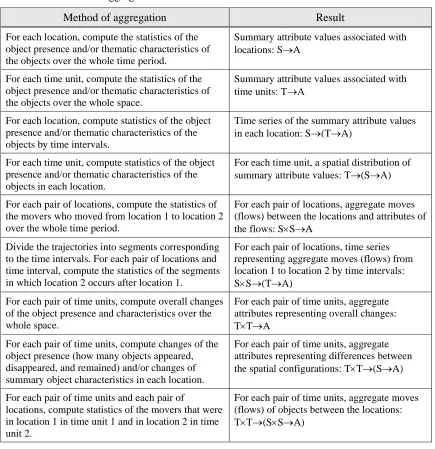
Table 1. Methods for aggregation of movement and event data.

Method of aggregation Result

For each location, compute the statistics of the object presence and/or thematic characteristics of the objects over the whole time period.

Summary attribute values associated with locations: S→A

For each time unit, compute the statistics of the object presence and/or thematic characteristics of the objects over the whole space.

Summary attribute values associated with time units: T→A

For each location, compute statistics of the object presence and/or thematic characteristics of the objects by time intervals.

Time series of the summary attribute values in each location: S→(T→A)

For each time unit, compute statistics of the object presence and/or thematic characteristics of the objects in each location.

For each time unit, a spatial distribution of summary attribute values: T→(S→A)

For each pair of locations, compute the statistics of the movers who moved from location 1 to location 2 over the whole time period.

For each pair of locations, aggregate moves (flows) between the locations and attributes of the flows: S×S→A

Divide the trajectories into segments corresponding to the time intervals. For each pair of locations and time interval, compute the statistics of the segments in which location 2 occurs after location 1.

For each pair of locations, time series representing aggregate moves (flows) from location 1 to location 2 by time intervals: S×S→(T→A)

For each pair of time units, compute overall changes of the object presence and characteristics over the whole space.

For each pair of time units, aggregate attributes representing overall changes: T×T→A

For each pair of time units, compute changes of the object presence (how many objects appeared, disappeared, and remained) and/or changes of summary object characteristics in each location.

For each pair of time units, aggregate attributes representing differences between the spatial configurations: T×T→(S→A)

For each pair of time units and each pair of

locations, compute statistics of the movers that were in location 1 in time unit 1 and in location 2 in time unit 2.

For each pair of time units, aggregate moves (flows) of objects between the locations: T×T→(S×S→A)

In aggregation, it is essential to be aware about the modifiable unit problem: the analysis results may depend on how the original units are aggregated (geographical sciences use the term “modifiable areal unit”) (Openshaw 1984). This refers not only to the sizes of the aggregates (scale effects) but also to their locations and composition from the smaller units (the delineation of the spatial compartments or the origins of the time intervals). Therefore, it is always advisable to test the sensitivity of any findings to the way of aggregation.

6 Taxonomy

of

approaches

to analyzing movement

6.1 Visualization and interaction

The established visualization techniques used for movement data as well as for spatio-temporal events are animated map and space-time cube (Andrienko et al. 2003, Kraak 2003, Kapler and Wright 2005). Both visualizations support the analysis tasks targeting the spatial and temporal characteristics of the objects (movers and events) and their relations to space and to time. Thematic characteristics of the objects can be shown in the same display by visual properties (colour, size, shape, etc.) of the graphical elements representing the objects. Alternatively, thematic characteristics may be shown by additional visualizations such as scatterplot, parallel coordinates, and time graph. Temporal bar chart, also known as Gantt chart, can represent temporal positions (lifetimes) of objects. One dimension of this display (typically horizontal) represents time. Objects are represented by bars positioned according to the lifetimes of the objects. Time-variant thematic characteristics can be represented by colours or shades of bar segments (Kincaid and Lam 2006).

Purely visual techniques may be ineffective when the number of movers is large and/or the time period under study is long. There are two basic approaches to dealing with large datasets. One is aggregation of the data and visualization of the aggregates obtained. Andrienko and Andrienko (2008) survey the existing methods for the aggregation of movement data and subsequent visualization. The visualization techniques include animated maps showing aggregated spatial configurations in different time units, maps with diagrams showing the temporal variation of aggregate attributes values in locations, temporal histogram portraying data aggregated by time intervals over the whole space, transition matrices and flow maps showing aggregate moves between locations.

Another approach to dealing with large amounts of data is selection (filtering) of the data, thus allowing only a small portion of the data satisfying current query conditions to be visualized. Thus, in the system described by Yu (2006), the user may formulate queries by referring to entities, their activities, and spatio-temporal relations, specifically, co-location in space, co-location in time, and co-existence, i.e. co-location in both space and time.

Table 2 describes the existing visualization methods applicable to detailed (i.e. not aggregated) movement data and event data. Table 3 describes the methods applicable to aggregated data. Here we explain some terms used in the descriptions of the visualization methods. Retinal properties (Bertin 1983) are non-positional visual properties of graphical elements: colour, size, shape, orientation, etc. Map sequence is a visualization consisting of multiple maps representing situations in different time units. This technique may be used in two forms: animated map (temporal arrangement of the individual maps) and “small

multiples” (spatial arrangement of the maps). Space-time graph is a two-dimensional display with one axis (typically horizontal) representing time and the other axis representing space as a finite linearly ordered set of locations. Spatio-temporal positions of objects are shown by points or bars placed in the display; trajectories may be represented by lines.

In addition to verbal descriptions, we represent the visualization techniques schematically by pictographs, borrowing the idea from Bertin (1983). The pictographs indicate what types of information are represented by the display dimensions and what information is shown within the display. Thus, in a map, two display dimensions are used to represent space. This is schematically represented by horizontal and vertical axes connected by an arc labelled with letter ‘S’.

A general note to the contents of Table 2 and Table 3 is that the visualizations should include information about the spatio-temporal context in which the events and/or object movements occur. Spatial context may be represented on spatial displays (maps) and spatio-temporal displays (space-time cube, map sequence). Temporal context may be represented on temporal displays, such as time graph and bar chart, and spatio-temporal displays.

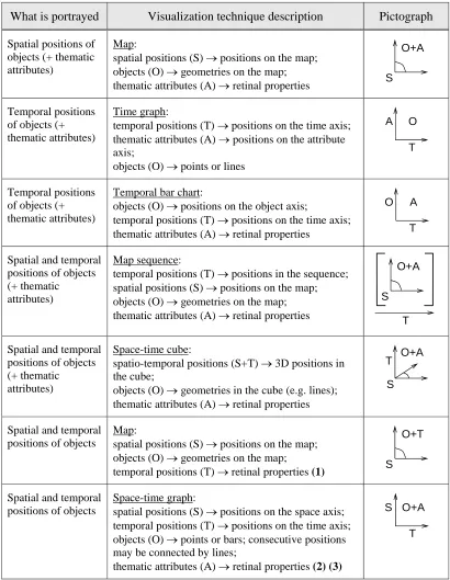
Table 2. Methods for visualization of detailed (not aggregated) movement and event data What is portrayed Visualization technique description Pictograph

Spatial positions of objects (+ thematic attributes)

Map:

spatial positions (S) → positions on the map; objects (O) → geometries on the map;

thematic attributes (A) → retinal properties S

O+A

Temporal positions of objects (+ thematic attributes)

Time graph:

temporal positions (T) → positions on the time axis; thematic attributes (A) → positions on the attribute axis;

objects (O) → points or lines

T

A O

Temporal positions of objects (+ thematic attributes)

Temporal bar chart:

objects (O) → positions on the object axis;

temporal positions (T) → positions on the time axis;

thematic attributes (A) → retinal properties T

O A

Spatial and temporal positions of objects (+ thematic attributes)

Map sequence:

temporal positions (T) → positions in the sequence; spatial positions (S) → positions on the map; objects (O) → geometries on the map; thematic attributes (A) → retinal properties

S O+A

T

Spatial and temporal positions of objects (+ thematic attributes)

Space-time cube:

spatio-temporal positions (S+T) → 3D positions in the cube;

objects (O) → geometries in the cube (e.g. lines); thematic attributes (A) → retinal properties

O+A

S T

Spatial and temporal positions of objects

Map:

spatial positions (S) → positions on the map; objects (O) → geometries on the map;

temporal positions (T) → retinal properties (1) S

O+T

Spatial and temporal positions of objects

Space-time graph:

spatial positions (S) → positions on the space axis; temporal positions (T) → positions on the time axis; objects (O) → points or bars; consecutive positions may be connected by lines;

thematic attributes (A) → retinal properties (2) (3)

Displacements (changes of spatial positions) of movers from one time unit to another

Map:

displacements (ΔS) → arrows connecting spatial positions;

thematic attributes (A) → retinal properties of the arrows S Δs(O)+A Displacements of movers between consecutive time units

Map sequence (one map per pair of time units): temporal positions (T1,T2) → positions in the

sequence;

displacements (ΔS) → arrows connecting spatial positions;

thematic attributes (A) → retinal properties T

S Δs(O)+A Displacements of movers between consecutive time units Space-time cube:

displacements (T1,T2,ΔS) → arrows connecting

spatial and temporal positions;

thematic attributes (A) → retinal properties of the arrows S T Δs(O)+A Displacements of movers between consecutive time units Space-time graph:

displacements (T1,T2,ΔS) → arrows connecting

spatial and temporal positions;

thematic attributes (A) → retinal properties (2) (3) T S

Δs(O)+A

Spatial aspect of trajectories

Map:

trajectories (Tr) → lines on the map;

static thematic attributes (A) → retinal properties of the whole lines;

time-dependent thematic attributes (A(t)) → retinal properties of line segments

S

Tr(O)+A

Spatial and temporal aspects of

trajectories

Space-time cube:

trajectories (Tr) → 3D lines in the cube;

static thematic attributes (A) → retinal properties of the whole lines;

time-dependent thematic attributes (A(t)) → retinal properties of line segments

S

T Tr(O)+A

Spatial and temporal aspects of the trajectories

Space-time graph:

spatial positions (S) → positions on the space axis; temporal positions (T) → positions on the time axis; consecutive positions of the same object are

connected by lines;

thematic attributes (A) → retinal properties of the lines (2) (3)

T S

Tr(O)+A

Notes:

(1)It is advisable to use this method after temporal generalization, which reduces the number of different time values to be visually distinguished.

(3)This display lacks spatial information. It should be linked to a spatial display, e.g. by brushing.

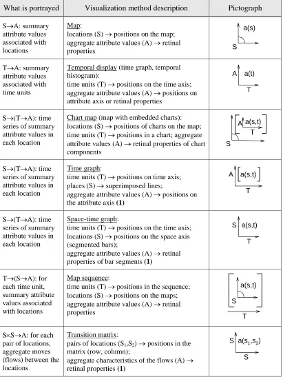
Table 3. Methods for visualization of aggregated movement and event data

What is portrayed Visualization method description Pictograph

S→A: summary attribute values associated with locations

Map:

locations (S) → positions on the map; aggregate attribute values (A) → retinal

properties S

a(s)

T→A: summary attribute values associated with time units

Temporal display (time graph, temporal histogram):

time units (T) → positions on the time axis; aggregate attribute values (A) → positions on attribute axis or retinal properties

T A a(t)

S→(T→A): time series of summary attribute values in each location

Chart map (map with embedded charts): locations (S) → positions of charts on the map; time units (T) → positions in a chart; aggregate attribute values (A) → retinal properties of chart components

S

T A a(s,t)

S→(T→A): time series of summary attribute values in each location

Time graph:

time units (T) → positions on time axis; places (S) → superimposed lines;

aggregate attribute values (A) → positions on the attribute axis (1)

T A a(s,t)

S→(T→A): time series of summary attribute values in each location

Space-time graph:

time units (T) → positions on the time axis; locations (S) → positions on the space axis (segmented bars);

aggregate attribute values (A) → retinal properties of bar segments (1)

T S a(s,t)

T→(S→A): for each time unit, summary attribute values associated with locations

Map sequence:

time units (T) → positions in the sequence; locations (S) → positions on the maps; aggregate attribute values (A) → retinal properties

S

T a(s,t)

S×S→A: for each pair of locations, aggregate moves (flows) between the locations

Transition matrix:

pairs of locations (S1,S2) → positions in the

matrix (row, column);

aggregate characteristics of the flows (A) → retinal properties (1)

S×S→A: for each pair of locations, aggregate flows between the locations

Flow map:

flows (S1,S2) → arrows connecting locations;

aggregate characteristics of the flows (A) →

retinal properties _S

a(s₁,s₂)

S×S→(T→A): for each pair of locations, time series of flows between the locations by time intervals

Flow map sequence, one map per time interval: temporal positions (T) of the intervals (ΔT) → positions in the sequence;

flows (S1,S2) → arrows connecting locations;

aggregate characteristics of the flows (A) → retinal properties of the arrows

S

a(s₁,s₂,Δt)

T

S×S→(T→A): for each pair of locations, time series of flows between the locations by time intervals

Space-time cube, possibly, with planes separating the time intervals (described by Andrienko and Andrienko 2007):

flows (S1,S2,ΔT) → arrows connecting positions

<location, time>;

aggregate characteristics of the flows (A) → retinal properties of the arrows

T

a(s₁,s₂,Δt)

S

S×S→(T→A): for each pair of locations, time series of flows between the locations by time intervals

Sequence of transition matrices, one matrix per time interval:

temporal positions (T) of the intervals (ΔT) → positions in the sequence;

pairs of places (S1,S2) → positions in the matrix

(row, column);

aggregate characteristics of the flows (A) → retinal properties (1)

T S S a(s1,s2,Δt)

S×S→(T→A): for each pair of locations, time series of flows between the locations by time intervals

Transition matrix with embedded charts: pairs of locations (S1,S2) → positions in matrix

(row, column);

time units (T) → positions in a chart; aggregate characteristics of the flows (A) → retinal properties of chart components (1)

S S

T a(s₁,s₂,t) A

S×S→(T→A): for each pair of locations, time series of flows between the locations by time intervals

Space-time graph:

flows (S1,S2,ΔT) → arrows connecting positions

<location, time>;

aggregate characteristics of the flows (A) →

retinal properties of arrows (1) T

S

a(s₁,s₂,Δt)

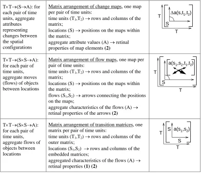
T×T→A: for each pair of time units, aggregate attributes representing overall changes

T-T-plot with two time axes (described by e.g. Imfeld 2000):

pairs of time units (T1,T2) → positions;

aggregate attribute values (A) → retinal properties

T×T→(S→A): for each pair of time units, aggregate attributes representing changes between the spatial configurations

Matrix arrangement of change maps, one map per pair of time units:

time units (T1,T2) → rows and columns of the

matrix;

locations (S) → positions on the maps within the matrix;

aggregate attribute values (A) → retinal properties of map elements (2)

S

T Δa(s,t₁,t₂) T

T×T→(S×S→A): for each pair of time units, aggregate moves (flows) of objects between locations

Matrix arrangement of flow maps, one map per pair of time units:

time units (T1,T2) → rows and columns of the

matrix;

locations (S) → positions on the maps within the matrix;

flows (S1,S2) → arrows connecting the positions

on the maps;

aggregate characteristics of the flows (A) → retinal properties of the arrows (2)

S

a(s₁,s₂,t₁,t₂)

T T

T×T→(S×S→A): for each pair of time units, aggregate flows of objects between locations

Matrix arrangement of transition matrices, one matrix per pair of time units:

time units (T1,T2) → rows and columns of the

outer matrix;

locations (S1,S2) → rows and columns of the

embedded matrices;

aggregated characteristics of the flows (A) → retinal properties (1) (2)

T T

S S a(s₁,s₂)

Notes:

(1)This display lacks spatial information. It should be linked to a spatial display, e.g. by brushing.

(2)Whilst this visualization is theoretically possible, we are not aware of existing

implementations. Generally, displays representing differences for all pairs of time units simultaneously are complex and hard to interpret. In practice, only differences between consecutive time moments are usually visualized.

6.2 Computational analysis methods

6.2.1 Clustering

Simple visualizations, queries, and aggregation may be insufficient for supporting synoptic tasks. Synoptic tasks often aim at gaining an overall concept and a concise description of a phenomenon. This corresponds to the notion of pattern used in data mining: “a pattern is an expression E in some language L describing facts in a subset FE of a set of facts F so that E is simpler than the enumeration of all facts in FE” (Fayyad et al. 1996). This definition suggests that a possible way to obtain a concise description, or pattern, is to unite the available facts into groups by similarity or closeness and then describe each group as a whole. Clustering is specifically meant for grouping items by similarity or closeness.

similarity/closeness among the items. The clustering techniques are represented by schematic expressions C(x|y), where x denotes the items grouped and y denotes the characteristics of the items used. The table also describes the synoptic tasks that can be supported by clustering in terms of their analysis targets.

Table 4. Synoptic tasks in movement analysis that can be supported by clustering Items to

group

Characteristics of the items

Schematic

representation Possible analysis targets

Events, movers

Positions in space and/or in time (+ thematic attributes)

C(O|S); C(O|T); C(O|S×T) C(O|S×A); C(O|T×A); C(O|S×T×A)

1) Spatio-temporal distribution of objects and their characteristics

2) Distance relations among objects: spatial, temporal, attributive (i.e. among attribute values)

Trajectories of movers Spatial, temporal, and/or thematic properties of trajectories C(Tr|S); C(Tr|T); C(Tr|S×T) C(Tr|A); C(Tr|S×A); C(Tr|T×A); C(Tr|S×T×A)

1) Distribution of spatial, temporal, and/or thematic characteristics of trajectories over space, time, and/or set of movers

2) Distance relations among trajectories: spatial, temporal, attributive

Locations Presence dynamics, time series of

attributes

C(S|(T→P(O))); C(S|(T→A))

Generic patterns (classes) of presence dynamics or attribute variation profiles and their distribution over space

Time units Spatial configurations, spatial distributions of attribute values

C(T|(S→P(O))); C(T|(S→A))

Generic patterns (classes) of spatial configurations or value distributions and their distribution over time

The most common way to visualize clustering results is colouring of display elements representing the clustered items according to their cluster membership. Another frequently used approach is showing each cluster separately, e.g. in a small multiples display. There are also approaches involving graphical summarization of clusters, e.g. generation of convex hulls (Buliung and Kanaroglou 2004) or aggregate flows (Andrienko and Andrienko 2010) from clusters of trajectories. Additionally to these, various statistics are computed for the clusters and represented by suitable graphs or charts.

6.2.2 Extraction of specific relations

Clustering may be helpful in investigating distance relations among elements of S, T, or O but not other kinds of relations. Since there are many possible kinds of relations, it is unfeasible to investigate all of them simultaneously. A synoptic task usually targets one kind of relation. In order to fulfil the task, it is often necessary first to find (extract) the occurrences of this kind of relation among the target elements. For this purpose, various ad hoc methods are devised, mostly in the area of data mining. It should be noted that the term ‘pattern’ is typically used in the data mining literature in the sense in which we use a more specific term ‘relation’.

(2005) finds occurrences of two kinds of spatio-temporal relations among movers,

synchronous movement and “trend setting”, when movements of some mover are repeated by other movers after a time lag. Giannotti et al. (2009) have developed a method to extract relations called “temporally annotated sequences”, or “T-patterns”. This is a kind of temporal relation among two or more locations that are visited in a particular sequence with particular transition times between the locations.

Relations between situations in different time units may be analysed by means of change detection techniques, which are developed in the areas of computer vision, image processing, and remote sensing. In particular, these techniques are used for the reconstruction of events, movers, and trajectories from images (e.g. Turdukulov et al. 2007, Höferlin et al. 2009). We are not aware of any specific computational techniques extracting relations of moving objects or events to elements of the spatial and temporal context; however, many kinds of such relations can be extracted by means of database queries (assuming that spatial and temporal predicates are supported).

The spatial and temporal positions of extracted relation occurrences can be visualized in the same way as spatial and temporal positions of events (in fact, relation occurrences are

events). Ad-hoc visualization techniques may be needed to visualize event-specific information, such as the transition times in temporally annotated sequences.

To refer to relation extraction techniques in the next section, we shall use the following codes: R(O×O) – extraction of relations among objects, R(S×S) – extraction of relations among places, and R(T×T) – extraction of relations among time units.

6.3 Correspondence between analysis tasks and methods

In this section, we link the types of analysis tasks to the visualizations, data transformations, and computational techniques that can support these tasks. Table 5 presents the links in a summarized way. The techniques are represented schematically: visualizations by pictographs (Section 6.1, Table 2), aggregations by formulas encoding the resulting data structures

(Section 5.6, Table 1), clustering by notations starting with C, such as C(O|S×T) (Section 6.2.1, Table 4), and relation extraction techniques by notations starting with R, such as R(O×O) (Section 6.2.2). For saving space, we include in Table 5 only the visualization techniques used for detailed (not aggregated) data. The techniques for aggregated data are chosen according to the data structures as specified in Table 3. We would like to remind that aggregation is not suitable for elementary level tasks.

The terms ‘spatial relations’, ‘temporal relations’, and ‘spatio-temporal relations’ have the following meanings (when no further specification is given):

ƒ Spatial relations = spatial relations to locations and spatial objects

ƒ Temporal relations = temporal relations to time units and temporal objects

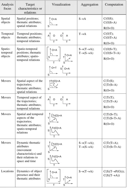
Table 5. Analysis tasks and respective supporting techniques. Analysis focus Target characteristics or relations

Visualization Aggregation Computation

Spatial objects

Spatial positions; thematic attributes;

spatial relations S

O+A S→A C(O|S);

C(O|S×A)

R(O×O)

Temporal objects

Temporal positions; thematic attributes;

temporal relations _T

A O

T

O A T→A C(O|T);

C(O|T×A)

R(O×O)

Spatio-temporal objects Spatio-temporal positions; thematic attributes; spatio-temporal relations S O+A T O+A S T S O+T T S O+A

S→(T→A); T→(S→A)

C(O|S×T); C(O|S×T×A)

R(O×O)

Movers Spatial aspect of the trajectories;

thematic attributes; spatial relations

S

Tr(O)+A C(Tr|S); C(Tr|S×A)

R(O×O)

Movers Temporal aspect of the trajectories; thematic attributes; temporal relations T A O T

O A C(Tr|T);

C(Tr|T×A)

R(O×O)

Movers Spatial and temporal aspects of the trajectories; thematic attributes; spatio-temporal relations S T Tr(O)+A T S Tr(O)+A

C(Tr|S×T); C(Tr|S×T×A)

R(O×O)

Movers Dynamic thematic

attributes (movement characteristics) and their relations to space and time

S

T Tr(O)+A

T S Tr(O)+A

S→(T→A); T→(S→A)

C(Tr|T×A); C(Tr|S×T×A)

Locations Dynamics of object presence and their thematic attributes _S

O+A

T

O+A

S T

S→(T→A) C(S|(T→P(O)));

S O+T

T S O+A

Locations Relations among locations

S

Δs(O)+A

T S

Δs(O)+A

S T

Δs(O)+A

T S

Δs(O)+A

S×S→A; S×S→(T→A)

R(S×S)

Time units

Spatial configurations, spatial distributions of attribute values

S O+A

T

T→(S→A) C(T|(S→P(O)));

C(T|(S→A))

Time units

Relations among time units

S T

Δs(O)+A

T S

Δs(O)+A

T×T→A; T×T→(S→A); T×T→(S×S→A)

R(T×T)

7 Examples

To illustrate the framework, we give an example of movement data, consider the possible analysis tasks, and describe a few tools implementing some of the generic analytic techniques from our taxonomy and supporting selected analysis tasks.

7.1 Data

The data we take is not a typical example of movement data dealt with in the research literature. At the first glance, they may even not be recognized as movement data. The data describe the geographically referenced photos from the Flickr photo-sharing Web site. The geographical positions are specified by the photo owners when they post the photos in Flickr. The times when the photos were taken can be retrieved from the metadata of the image files. Many Flickr users repeatedly post their georeferenced photos taken in different places and at different times. The geographic locations and times of the photos reflect the movements of the photographers (i.e. Flickr users who published the photos). Hence, this is an example of

publicly available API. In the following examples, we use a subset of the data referring to the territory of Switzerland and the period from January 1, 2005 to September 30, 2009.

In terms of our general framework, the Flickr users who publish georeferenced photos are the

movers. The sequence of the photo taking events of one mover makes the trajectory of this mover. The locations are the spatial positions of the events, which are originally specified as points (by geographical coordinates). By applying spatial generalization, we may generate a discrete set of areas, which will be considered as locations instead of the original points. Depending on the desired temporal scale of analysis, we may choose time intervals of different lengths as time units.

Besides the positions of the movers, the data also describe the photo taking events. Each event has its positions in space and time and some thematic attributes: image URL, count of the times the image was viewed, title, and list of tags. However, there are also other kinds of events that can be extracted from the data, in particular, events of several Flickr users being in the same location at the same time. These events may be related to other events that occurred in the real world and attracted attention of people: festivals, shows, parties, unusual natural phenomena, etc. They constitute a part of the context in which the movement and activities of the Flickr users take place. The context also includes the static geographic environment with the cities, natural areas, landmarks, etc., and events that have no particular positions in space, for example, public holidays. While the Flickr photos data do not directly describe the context, some information about the context is contained in the titles of the photos. Additional information may be retrieved from available maps representing the geographical environment and from the Web, as will be demonstrated in the following.

7.2 Tasks

Table 6 describes the types of tasks for which the Flickr photos data can be used. Table 6. The types of tasks in analyzing Flickr photos data.

Focus Target characteristics or relations

Elementary tasks Synoptic tasks

Photo taking events

Spatio-temporal positions; relations to locations, times, and context

Positions and relations of particular photos

Spatio-temporal distribution of a set of photos; relations of the distribution to the context

Photo taking events

Spatio-temporal relations among events

Relations (distance, direction) among particular photos

Occurrences of particular types of relations (e.g. concentrations in space and/or time) and their distribution in space and time

Movers (Flickr users)

Trajectories; relations to locations, times, and context

Trajectories and relations of particular photographers

Variety of spatial, temporal, and thematic characteristics of

trajectories, their spatial, temporal, and frequency distributions and relations to the context

Movers (Flickr users)

Spatio-temporal relations among movers

Relations among

particular photographers, e.g. proximity, joint travels, similar routes

Occurrences of particular types of relations (e.g. proximity, joint travels, similar routes), their characteristics and distribution in space and time

relations to context particular locations and their relations to context

dynamics (e.g. random

fluctuations, seasonal variation, regular peaks, irregular peaks), their spatial distribution and relations to the context

Locations Relations among locations

Relations among particular locations, e.g. common visitors, sequence of visiting

Occurrences of particular types of relations (e.g. common visitors, sequence of visiting), their characteristics and distribution in space and time

Time units

Spatial configurations; relations to context

Spatial configurations of photos or people in particular time units and their relations to context

Variety of patterns of spatial configurations (e.g. sets of actively visited places), their temporal distribution and relations to context

Time units

Relations among time units

Relations among particular time units, e.g. how the presence differs across the locations, where people moved

Occurrences of particular types of relations (e.g. sudden increase of presence in some/many locations), their characteristics and

distribution in space and time

7.3 Tools

In this subsection, we give examples of tools or tool combinations that can support two types of synoptic tasks selected from Table 6:

(1)Spatio-temporal distribution of a set of photos; relations of the distribution to the context (table row 1).

(2)Variety of spatial characteristics of trajectories, their spatial and frequency distributions and relations to the spatial context (table row 3; we focus only on the spatial aspect). The tools have been earlier described in other papers. Here we briefly demonstrate their application to the Flickr photos data.

7.3.1 Investigating the spatio-temporal distribution of photos

In the original data, the positions are specified by geographic coordinates. We apply spatial generalization to obtain a discrete set of locations (Andrienko and Andrienko 2010): We perform spatial clustering of the events and apply Voronoi tessellation of the territory (Okabe et al. 2000) using the centroids (mass centres) of the clusters as the generating points of the cells. The cells (polygons) are treated as the locations of the photos in the further analysis. We use the visualization technique Growth Ring Map (Bak et al. 2009). According to our classification (Table 2), this is a method in which spatial positions are represented by positions on a map and temporal positions by retinal properties. There is a note that this method should be preferably used after temporal generalization, which reduces the number of different time values to be visually distinguished. We apply the following temporal