A generalized linear model with smoothing effects for claims reserving

City, University of London Institutional Repository

Citation:

Bjorkwall, S., Hossjer, O., Ohlsson, E. and Verrall, R. J. (2011). A generalized

linear model with smoothing effects for claims reserving. Insurance: Mathematics and

Economics, 49(1), pp. 27-37. doi: 10.1016/j.insmatheco.2011.01.012

This is the unspecified version of the paper.

This version of the publication may differ from the final published

version.

Permanent repository link:

http://openaccess.city.ac.uk/3842/

Link to published version:

http://dx.doi.org/10.1016/j.insmatheco.2011.01.012

Copyright and reuse: City Research Online aims to make research

outputs of City, University of London available to a wider audience.

Copyright and Moral Rights remain with the author(s) and/or copyright

holders. URLs from City Research Online may be freely distributed and

linked to.

A generalized linear model with smoothing effects for claims

reserving

Susanna Bj¨orkwall∗,a_{, Ola H¨ossjer}a_{, Esbj¨orn Ohlsson}b_{, Richard Verrall}c

a

Department of Mathematics, Division of Mathematical statistics, Stockholm University, SE-106 91 Stockholm, Sweden

b

L¨ansf¨ors¨akringar Alliance, SE-106 50 Stockholm, Sweden

c

Cass Business School, City University, 106 Bunhill Row, London EC1Y 8TZ, United Kingdom

Abstract

In this paper, we continue the development of the ideas introduced in England & Verrall (2001) by suggesting the use of a reparameterized version of the generalized linear model (GLM) which is frequently used in stochastic claims reserving. This model enables us to smooth the origin, development and calendar year parameters in a similar way as is often done in practice, but still keep the GLM structure. Specifically, we use this model structure in order to obtain reserve estimates and to systemize the model selection procedure that arises in the smoothing process. Moreover, we provide a bootstrap procedure to achieve a full predictive distribution.

Key words: Bootstrap, Generalized linear model, Model selection, Smoothing, Stochastic claims

reserving

∗_{Corresponding author.}

Email address: [email protected] Phone number: +46-70-434 7680 Fax: +46-8-612 6717

1 INTRODUCTION 2

1. Introduction

Many stochastic claims reserving methods have now been established, see, for example, W¨utrich

& Merz (2008) and England & Verrall (2002). However, many actuaries use intuitive approaches

in conjunction with a standard reserving method, and it is necessary for stochastic methods to

also enable these to be used. One such intuitive method is the subject of this paper, which is to

allow some smoothing to be applied to the shape of the development pattern.

In Bj¨orkwall et al. (2009) an example of a deterministic development factor scheme, which is

frequently used in practice, was provided. This approach could be varied in many different ways

by the actuary depending on the particular data set under analysis. This includes smoothing the

development factors, perhaps after excluding the oldest observations and outliers. In this way the

impact of irregular observations in the data set is reduced and more reliable reserve estimates are

obtained. A common approach is to use exponential smoothing by log-linear regression of the

development factors, but other curves could be applied too, see Sherman (1984). These could also

be carried over to a bootstrap procedure in order to obtain the corresponding prediction error as

well as the predictive distribution, whose size and width, respectively, can be changed according

to the amount of smoothing and extrapolation.

Despite the intuitiveness and transparency of this approach it is certainly accompanied by some

statistical drawbacks. For instance, the statistical quality of the reserve estimates is not

opti-mal since they are not maximum likelihood estimators. Moreover, bootstrapping requires some

stochastic model assumptions anyway. When this model is defined at the resampling stage, rather

than at the original data generation stage the resulting reserving exercise leads to somewhat ad hoc

decisions and more subjectiveness compared to a more systematic methodology, where a stochastic

model is defined from start.

England & Verrall (2001) presented a Generalized Additive Model (GAM) framework of stochastic

claims reserving, which has the flexibility to include several well-known reserving models as special

cases as well as to incorporate smoothing and extrapolation in the model-fitting procedure. Using

1 INTRODUCTION 3

to the amount of smoothing, the error distribution and how far to extrapolate, then the fitted

model automatically provides statistics of interest, e.g. reserve estimates, measures of precision

and tests for goodness-of-fit. Such an approach is appealing, partly due to its statistical qualities

and partly in order to obtain a tool for selection and comparison of models, which then could be

systemized.

Recently Antonio & Beirlant (2008) applied a similar approach using a semi-parametric regression

model which is based on a generalized linear mixed model (GLMM) approach. However, both

GAMs and GLMMs might be considered as too sophisticated in order to become popular in

reserving practice.

In this paper, we instead suggest the use of a reparameterized version of the popular Generalized

Linear Model (GLM) introduced in a claims reserving context by Renshaw & Verrall (1998). This

model enables us to smooth origin, development and calendar year parameters in a similar way as is

often done in practice, but still keep a GLM structure which we can use to obtain reserve estimates

and to systemize the model selection procedure that arises in the smoothing process. While

England & Verrall (2001) used the GAM in order to analytically compute prediction errors we

instead implement a bootstrap procedure to achieve a full predictive distribution for the suggested

GLM in accordance with the method developed in Bj¨orkwallet al.(2009).

The paper is set out as follows. The notation and a short summary of existing smoothing

ap-proaches, which to a large extent is based on the work of England & Verrall (2001, 2002), are

given in Section 2. The suggested model is introduced in Section 3, which also contains three

examples on how it can be used; one of them is the main topic of this paper. In Section 4 we

discuss model selection and some criteria are provided. The estimation of the parameters and the

reserving algorithm are described in Section 5, while Section 6 contains the bootstrap procedure.

2 SMOOTHING MODELS IN CLAIMS RESERVING 4

2. Smoothing models in claims reserving

2.1. Notation

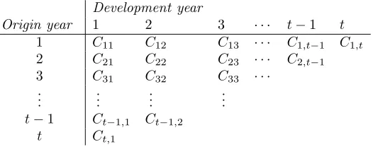
Let{Cij;i, j∈ ∇} denote the incremental observations of paid claims, which are assumed to be

available in a development triangle∇={(i, j);i= 1, . . . , t;j = 1, . . . , t−i+ 1}. The suffixesiand j refer to the origin year and the development year, respectively, see Table 2.1. In addition, the

suffixk=i+j is used for the calendar years, i.e. the diagonals of∇. Letn=t(t+ 1)/2 denote the number of observations.

Development year

Origin year 1 2 3 · · · t−1 t

1 C11 C12 C13 · · · C1,t−1 C1,t

2 C21 C22 C23 · · · C2,t−1

3 C31 C32 C33 · · ·

..

. ... ... ...

t−1 Ct−1,1 Ct−1,2

t Ct,1

Table 2.1:The triangle∇of observed incremental payments.

The purpose of a claims reserving exercise is to predict the sum of the delayed claim amounts in the

lower, unobserved future triangle{Cij;i, j∈∆}, where ∆ ={(i, j);i= 2, . . . , t;j=t−i+2, . . . , t},

see Table 2.2. We writeR=P_∆Cij for this sum, which is the outstanding claims for which the

insurance company must hold a reserve. The outstanding claims per origin year are specified by

summing per origin yearRi=Pj∈∆iCij, where ∆i denotes the row corresponding to origin year

iin ∆.

Development year

Origin year 1 2 3 · · · t−1 t

1

2 C2,t

3 C3,t−1 C3,t

..

. ... ...

t−1 Ct−1,3 · · · Ct−1,t−1 Ct−1,t

t Ct,2 Ct,3 · · · Ct,t−1 Ct,t

2 SMOOTHING MODELS IN CLAIMS RESERVING 5

Estimators of the outstanding claims per origin year and the grand total are obtained by ˆRi = P

j∈∆i

ˆ

Cij and ˆR=P∆Cˆij, respectively, where ˆCij is a prediction of Cij. With an underlying

stochastic reserving model, ˆCij is a function of the estimated parameters of that model, typically

chosen to make it an (asymptotically) unbiased predictor ofCij.

2.2. A deterministic development factor method

This section contains an example of how the chain ladder development factors might be smoothed

and extrapolated into a tail according to a deterministic algorithm.

The chain-ladder and other development factor methods operate on cumulative claim amounts

Dij= j X

ℓ=1

Ciℓ. (2.1)

Letµij=E(Dij). Development factors

fj = Pt−j

i=1µi,j+1

Pt−j i=1µij

, (2.2)

wherej = 1, . . . , t−1, are estimated for a fully non-parametric model without any smoothing of parameters by

ˆ fj=

Pt−j i=1Di,j+1

Pt−j i=1Dij

. (2.3)

By examining a graph of the sequence of ˆfj’s the actuary might decide to smooth them, for

instance, for j ≥ 4. Exponential smoothing could be used for that purpose, i.e. the ˆfj’s are

replaced by estimators obtained from a linear regression of ln( ˆfj−1) on j. By extrapolation in

the linear regression this also yields development factors for a tail j = t, t+ 1. . . , t+u. The

original ˆfj’s are kept forj <4 and the smoothed ones used for allj ≥4. Let ˆfjsdenote the new

sequence of development factors. Estimates ˆµij for ∆ can now be computed as in the standard

chain-ladder method yielding

ˆ

µij =Di,t−ifˆts−ifˆts−i+1. . .fˆjs−1 (2.4)

and

ˆ

2 SMOOTHING MODELS IN CLAIMS RESERVING 6

Note that the truncation pointj= 4 of the unsmoothed development factors, has to be decided by

eye. Moreover, this approach could be varied, the actuary might choose, for example, to disregard

some of the latest development factors for the regression procedure and then more decisions have to

be made. Hence, this approach is quite ad hoc. A more stringent methodology requires a stochastic

model for the claims, see Verrall & England (2005) and Verrall (2007) for more discussion.

2.3. Lognormal models

Early smoothing models applied to claims reserving were parametric and, for simplicity, normal

distributions were assumed. The usual assumptions were thatCij are independent with

ln(Cij) =ηij+ǫij, (2.6)

where ηij =E(ln(Cij)) andǫij ∼N(0, σ2). Hence, Cij ∼ LN(ηij, σ2), where N and LN denote

normal and lognormal distributions, respectively. Moreover, two models,

ηij=c+αi+βj (2.7)

and

ηij =c+αi+βi lnj+γij , (2.8)

were suggested.

Model (2.7) was introduced by Kremer (1982). Model (2.8), which is referred to as the Hoerl

curve, can be ascribed to Zehnwirth (1985), see e.g. England & Verrall (2001). The original

document does no longer exist according to Insureware even though it is frequently referred to

in the literature. However, the Hoerl curve is also mentioned in the conference paper Zehnwirth

(1989). This model was popular since it often provides a reasonable approximation to the shape

of the payment pattern; it starts with a rapidly increasing peak and then decays exponentially.

Moreover, it can be used for extrapolation of a tail of payments beyondt.

De Jong & Zehnwirth (1983) used the Kalman filter in order to smooth the estimates of the

parametersβi andγi in (2.8) according to a framework for a family of models. Verrall (1989) also

2 SMOOTHING MODELS IN CLAIMS RESERVING 7

Barnett & Zehnwirth (2000) introduced a model which is referred to as the probabilistic trend

family (PTF), and this model could be expressed using

ηij=αi+ j−1

X

l=1

βl+ i+_Xj−1

k=2

γk (2.9)

in (2.6). Here the βl’s and γk’s account for linear trends between the development years and

calendar years, respectively.

2.4. Generalized linear models

Wright (1990) introduced a parametric alternative which is based on a risk theoretic model

includ-ing the assumption of Poisson distributed claim numbers and gamma distributed claim amounts.

The model can be expressed as a GLM

E(Cij) =mij and V ar(Cij) =φijmpij

ln(mij) = ηij, (2.10)

where

ηij=uij+c+αi+βi lnj+γij+δk , (2.11)

and p= 1, see e.g. England & Verrall (2001) for the derivation. The termuij is a known offset,

a function of an exposure and a known adjustment term, see Wright (1990), whileδk allows for

claims inflation. It is easy to see that (2.11) is similar to the Hoerl curve in (2.8), but the relation

between the responses and the predictor differs. Moreover, the error distribution no longer has to

be normal. Wright (1990) used the Kalman filter to produce smoothed estimates of the parameters.

Renshaw & Verrall (1998) used (2.7) in (2.10) and related the model to the chain-ladder method

for p= 1. Note that the scale parameter is usually assumed to be constant in this context, i.e.

φij =φ, and, hence, we will stick to this assumption from now on.

Equation (2.7) can be extended to include a calender year parameter according to

3 GLM WITH LOG-LINEAR SMOOTHING 8

However, the number of parameters is then usually too large compared to the small data set of

aggregated individual paid claims in Table 2.1. In any case, a side constraint, e.g.

α1=β1=γ2= 0 (2.13)

is needed to estimate thev= 3t−2 remaining model parametersc, αi,βj andγk, typically under

the assumptionp= 1 orp= 2, corresponding to an over-dispersed Poisson (ODP) distribution or

a gamma distribution, respectively. Note that it is only possible to estimate γk fork = 3, . . . , t,

while a further assumption is needed regarding the futurek=t+ 1, . . . ,2t.

2.5. Generalized additive models

GAMs, which include non-parametric smoothers, are an alternative in order to obtain more

flexibil-ity than parametric smoothing models can provide. Using this approach, Verrall (1996) extended

the model in (2.10) and (2.7) to incorporate smoothing of the origin year parametersαi. England

& Verrall (2001) extended that idea further by creating a general framework which can express

several previous reserving models as special cases. The framework was then used, among other

things, to allow for smoothing over the development year parameterβj, in (2.10) and (2.7), too.

2.6. Generalized linear mixed models

Antonio & Beirlant (2008) presented a semi-parametric regression model which is based on a

GLMM approach. Using a Bayesian implementation they extended the work of England & Verrall

(2001) to include simulation of predictive distributions. In addition, the suggested model could

be used for more complicated data sets involving e.g. quarterly development or longitudinal data.

3. GLM with log-linear smoothing

3.1. A general parametrization

In this section we introduce a matrix representation of equation (2.12) according to

3 GLM WITH LOG-LINEAR SMOOTHING 9

usingθf ull= c α β γ T and η= η11 . . . η1t η21 . . . η2,t−1 . . . ηt1 T, where

α = α2 . . . αt , β = β2 . . . βt , γ = γ3 . . . γt+1 . Recall that the number of

observations in∇Cisn=t(t+ 1)/2, which is also the length ofη. Moreover,Xf ull is the design

matrix of the system. The index ’full’ refers to the GLM in (2.10) and (2.12) which from now on

will be considered asfull in contrast to the subsequent smoothed version.

In order to smooth thev= 3t−2 original parametersαi,βjandγk and, hence, reparametrize the

system (3.1) we introduce a new set of parametersa= a1 . . . aq

,b= b1 . . . br

and

g= g1 . . . gs

, where 0≤q, r, s≤t−1. Let

a A = α

b B = β

gΓ = γ, (3.2)

which corresponds to

a1 . . . aq

  

A12 . . . A1t

..

. ... ... Aq2 . . . Aqt

 

= α2 . . . αt

(3.3)

b1 . . . br

  

B12 . . . B1t

..

. ... ... Br2 . . . Brt

 

= β2 . . . βt

(3.4)

g1 . . . gs   

Γ13 . . . Γ1,t+1

..

. ... ... Γs3 . . . Γs,t+1

 

= γ3 . . . γt+1 . (3.5)

Moreover, letθ= c a b g T, containingw= 1 +q+r+sparameters. We can now express

θf ullas

θf ull=D θ =    

1 0 0 0

0 A 0 0

0 0 B 0

0 0 0 Γ

    T θ (3.6)

using the blocksA,B andΓin (3.2) - (3.5). The matrixD is of dimensionv×w.

Finally (3.1) can be rewritten using the new parameters

3 GLM WITH LOG-LINEAR SMOOTHING 10

whereX is the new design matrix.

Example 1: The full GLM. If q = r = s = t−1 and A = B = Γ = I, where I is the identity matrix, we get the full GLM. However, if we choose other values ofq,r, sandA,B,Γ,

respectively, we will still keep a GLM structure.

Example 2: A Hoerl curve. A special case of the Hoerl curve in (2.8), where βi = β and

γi=γ, can be expressed according to (3.7) usingβ= β γ ,Γ=0,

θ= c α2 . . . αt β γ T

and

D=

        

1 0 . . . 0 0 0 0 1 . . . 0 0 0 0 0 . . . 1 0 0 0 0 . . . 0 ln(1) 1

..

. ... ... ... ... ... 0 0 . . . 0 ln(t) t

        

.

Hence,q=t−1,r= 2 and s= 0. Note that there is an overlap in the naming of parameters in (2.8) and (3.1).

3.2. The log-linear smoothing model

In this section, we consider the GLM which is studied in the remainder of this paper. For smoothing

purposes, curves such as the following are of interest:

αi = ai−1; 2≤i≤q

αi = aq−1+aq(i−q) ; q+ 1≤i≤t

βj = bj−1; 2≤j ≤r (3.8)

βj = br−1+br(j−r) ; r+ 1≤j≤t

γk = gk−1; 2≤k≤s

γk = gs−1+gs(k−s) ; s+ 1≤k≤t ,

where 1≤q, r, s≤t−1. For definiteness,a0= 0,b0= 0 andg0= 0 in the second, fourth and sixth

equations whenq= 1,r= 1 ands= 1, respectively. Moreover, note thata1, . . . , aq−1,b1, . . . , br−1

3 GLM WITH LOG-LINEAR SMOOTHING 11

The amount of smoothing can now be set by the choice ofq, r ands. Note that this has some

similarities to the ad hoc procedure described in Section 2.2. For instance, model (3.8) could be

used in order to smooth the later part of the run-off pattern and perhaps extendβj beyondt for

a tail. It might not make sense to do the same forαi, however, the model could be useful in order

to forecast calendar year effects by extrapolation ofγk. The key to this is the choice ofq, rand

s, and we will set out an automatic way to do this, to replace the ad hoc procedure often used.

3.2.1. A special case: Smoothing of the run-off pattern

From now on we will stick to the assumptionq=t−1,s= 0 and Γ=0 in (3.8). Thus,D will be of size (2t−1)×(t+r),

D=             

1 0 . . . 0 0 . . . 0 0 0 1 . . . 0 0 . . . 0 0

..

. ... ... ... ... ... ... ... 0 0 . . . 1 0 . . . 0 0 0 0 . . . 0 1 . . . 0 0

..

. ... ... ... ... ... ... ... 0 0 . . . 0 0 . . . 1 t−r

             . (3.9)

This special case is particularly interesting since it can be related to the log-linear smoothing of

chain-ladder development factors in Section 2.2.

The theoretical development factors in equation (2.2) can be rewritten as

fj= Pt−j

i=1

Pj+1

l=1mil Pt−j

i=1

Pj l=1mil

, (3.10)

wheremij is defined by the underlying GLM structure in (2.10), (3.1) and (3.8). Recall that the

observed development factors

ˆ fj=

Pt−j i=1

Pj+1

l=1mˆil Pt−j

i=1

Pj l=1mˆil

(3.11)

4 MODEL SELECTION 12

Thus,

ln (fj−1) = ln

Pt−j i=1

Pj+1

l=1ec+αi+βl

Pt−j i=1

Pj

l=1ec+αi+βl

−1

!

= ln

Pj+1

l=1eβl

Pj l=1eβl

−1

!

= βj+1−ln

j X

l=1

eβl

!

. (3.12)

Forj≥requation (3.12) can be written as

ln (fj−1) = bp+bp−1(j+ 1−q+ 1)−ln

j X

l=1

eβl

!

. (3.13)

Sinceris supposed to be so large that the linear extrapolation captures the tail only small values

of βj will remain to the right of r. Therefore the linear parametrization of βj approximately

leads to log-linear smoothing of theoretical development factors fj, analogous to the log-linear

smoothing of true development factors accounted for in Section 2.2. A numerical comparison of

the two approaches is provided in Section 7.2.

4. Model selection

In practice, we would like to select the truncation pointsq, randsof Section 3.2 from data. To

this end, we let _θˆ_{qrs denote the estimated parameter vector for a model with fixed (q, r, s). We}

can choose the model

(ˆq,r,ˆ sˆ) = argmin(q,r,s)∈ICrit(θˆqrs), (4.1)

that minimizes a model selection criterion Crit(_θˆ_{qrs) among a pre-chosen setIof candidate models.}

We then takeθˆ(ˆq,r,ˆˆs) as the final parameter estimators on which to base reserves.

An ad hoc GLM claims reserving approach would correspond to using a single modelI={(q, r, s)}. This is often what is done in practice, but it requires prior knowledge of the truncation pointsq,

r and s, which is often not realistic. Indeed, there are many situations when several candidate

models should be allowed for. For instance, suppose smoothing of development years is of concern,

whereas accident years are not smoothed and inflation not included in the model, then

4 MODEL SELECTION 13

is of interest. If we also allow the possibility of the last accident year parameter being linearly

interpolated from the previous two, we put

I={(t−2,1,0), . . . ,(t−2, t−1,0),(t−1,1,0). . . . ,(t−1, t−1,0)}. (4.3)

A linear inflation trend can be incorporated into either of (4.2) and (4.3) by simply replacings= 0

withs= 1 everywhere, and so on.

Note that low values ofr, where the most extreme choice would ber= 1, are not of any actual

in-terest in (4.2) and (4.3), however, we still choose to include them for completeness and illustration,

see Section 7.2.

In connection with (4.2), the classical exponential smoothing looks at the chain ladder estimated

development factors and then choosesI to contain one single model (t−1, r,0), where r is the visually determined break point for a linear trend on the log scale.

Akaike’s Information Criterion (AIC) and the Bayesian Information Criterion (BIC) could be used

as model selection criteria when working with likelihood functions. The definitions are

Crit = AIC(θˆqrs) = 2w−2l(θˆqrs) (4.4)

and

Crit = BIC(θˆqrs) = ln(n)w−2l(θˆqrs), (4.5)

see e.g. Miller (2002). Here w = 1 +q+r+s is the number of parameters and l(θˆqrs) is the

maximized log-likelihood function with respect to model (q, r, s). It can be seen that AIC and

BIC differ in that they penalize the fitted log-likelihood of large models in different ways.

Bootstrapping could also be used to estimate the mean squared error of prediction MSEP( ˆR) =

E(R−Rˆ)2_{, where the expected value is with respect to R and ˆR. Estimating MSEP by}

bootstrapping, we get a model selection criterion

Crit =M SEPd (θˆqrs) =E

(R∗∗_−Rˆ∗₎2_{, (4.6)}

where R∗∗ _{and ˆR}∗ _{are resampled reserves and resampled estimated reserves, respectively. The}

5 ESTIMATING THE MODEL PARAMETERS 14

the criterion BOOT in Pan and Le (2001). Note that M SEPd measures the deviation between

the future claims and the predicted ones under a certain model, while AIC and BIC measure the

deviation between the observations and their expected values.

Another possibility, pursued by Pan (2001), is to define an analogue of AIC, where the likelihood

is replaced by the quasi-likelihood function Q(θ) of Wedderburn (1974). Pan (2001) suggested a

quasi-likelihood information criterion

QIC(θˆqrs) = 2 trace(Ω ˆˆV)−2Q(θˆqrs), (4.7)

where_Ωˆ ₌₋∂2

∂θ2Q(θ)|θ₌θˆ_qrs andVˆ is an estimator ofV = Cov(θˆqrs), see Liang & Zeger (1986) for an example. Note that QIC reduces to AIC when the quasi and true likelihoods coincide, since

thenΩˆ =Vˆ−1.

England & Verrall (2001) discuss the use of the deviance for model comparison in their GAM

framework. They remark that it is not obvious how many degrees of freedom should be used since

the GAM smoothers are non-parametric. Here, on the other hand, the deviance is inappropriate

since it does not penalize large models and, hence, it will by definition be lower for larger models.

Note that the outcome of the model selection is sensitive to the chosen criterion. For instance,

AIC usually tends to select large models. Moreover, the suggested criteria do not help us choose

among the underlying distributional assumptions. In Section 7 we will illustrate model selection

numerically using AIC, BIC andM SEPd as criteria for the special case in Section 3.2.1.

5. Estimating the model parameters

Here the estimation procedure for the special case in Section 3.2.1 is described, which could be

extended to consider the general model in Section 3.2.

5.1. Estimation ofφfor model selection

Care must be taken regarding the choice of estimator ˆφ, since it will strongly affect the outcome of

5 ESTIMATING THE MODEL PARAMETERS 15

i.e. (t−1, r,0) wherer < t−1, can be expressed as a sum of two terms; the random errors of the full model (t−1, t−1,0) and a second termmf ull_ij −mij, which accounts for systematic effects

not captured by the smaller model. Hence, estimatingφfor each model (t−1, r,0) yields a higher value compared to estimatingφbased on the full model (t−1, t−1,0).

For model selection using AIC and BIC in (4.4) and (4.5) we are interested in comparing the

random errors of the models. Therefore the estimator of φ should be based on the full model,

see e.g. Pan (2001). However, if we use bootstrapping, as in (4.6), the systematic effects of

model (t−1, r,0) should be included, otherwise smaller models will benefit since M SEP would be underestimated.

Hence, in order to estimateφfor AIC and BIC we use the Pearson residuals

rf ull_ij = Cij−mˆ

f ull ij r

ˆ mf ull_ij p

(5.1)

and forM SEPd we use

rij=

Cij−mˆij q

ˆ mpij

, (5.2)

where ˆmij is the estimator ofmij for the particular model under analysis. This yields

ˆ

φf ull₌ 1

n−2t+ 1

X

∇

(rf ull_ij )2, (5.3)

and, sincew= 1 +q+r+s= 2t−1 is the number of estimated parameters (excluding ˆφ) in the full model (t−1, t−1,0),

ˆ φ= 1

n−w

X

∇

(rij)2. (5.4)

Here, the index ’full’ is only used for clarity.

5.2. The reserving algorithm

We can now implement a log-linear smoothing procedure for the reserving exercise according to

the following scheme.

1. Define the design matrixX_{f ull} of the full model in (3.1) when the GLM in (2.10) and (2.7)

6 BOOTSTRAP AND QUANTILE PREDICTION 16

2. Define a family I of models, based on truncation points (t−1, r,0), that we would like to select a model from.

FOR all (t−1, r,0)∈I DO:

3. CreateAand B, and hence, the block matrixD.

4. CalculateX=Xf ullD.

5. Set up the new GLMη =X θ. Then use some standard software to compute an estimate

ˆ

θt−1,r,0 ofθ=θt−1,r,0 by maximizing e.g. the likelihood or quasi likelihood.

6. Evaluate the chosen model selection criterion Crit(θˆt−1,r,0) for model (t−1, r,0) using either

(5.3) for AIC, BIC and QIC in (4.4), (4.5) and (4.7) or (5.4) for M SEPd in (4.6).

END.

7. Select model (t−1,ˆr,0) as in (4.1).

8. Obtain estimatorsEb(Cij) = ˆmijandV ard(Cij) = ˆφmˆpij from (2.10) and (2.7), withc,αiand

βj replaced by estimates, computed from the first four equations of (3.8) andθˆt−1,r,ˆ0. Here

ˆ

φis obtained from (5.4)

6. Bootstrap and quantile prediction

It is now straightforward to implement a bootstrap procedure for either the model_θˆ_t

−1,ˆr,0selected

by the reserving algorithm in Section 5.2 or for the full modelθˆt−1,t−1,0corresponding to the GLM

in (2.10) and (2.7). Including the model selection part in the bootstrap procedure implies that

each resampled pseudo-triangle is being individually analyzed in the bootstrap world in a similar

way as it had been by the actuary if it was an observed triangle in the real world. Hence, if there

are outliers in the data set the prediction error could decrease compared to the situation when

we less accurately apply the same reserving algorithm to all pseudo-triangles. It is difficult to

implement such a procedure for the deterministic approach in Section 2.2 since the truncation

points for the smoothing of the development factors usually is based on an ad hoc decision instead

of a systematic one.

We will use the bootstrap technique provided in Bj¨orkwallet al. (2009) for the implementation.

However, since it is beyond the scope of this paper to compare bootstrap algorithms we will focus

7 NUMERICAL STUDY 17

Hence, in addition to the assumptions in (2.10) and (2.7) we assume a full distributionF forCij,

parameterized by the mean and variance, so that we may writeF =F(mij, φmpij). Typically we

assume that F is either an ODP or a gamma distribution corresponding to p = 1 and p = 2,

respectively. We draw C∗

ij from F( ˆmij,φˆmˆpij), where ˆmij is calculated according to the model

(t−1,ˆr,0) selected as in (4.1), for all i, j ∈ ∇ and ˆφis obtained from (5.4). This produces the pseudo-triangles∇C∗_{. Steps 1-8 in Section 5.2 are then repeated for each∇C}∗ _{and the bootstrap}

estimates ˆR∗

i = P

j∈∆imˆ ∗

ij and ˆR∗= P

∆mˆ∗ij are finally calculated for each pseudo-triangle.

In order to get R∗∗

i = P

j∈∆iC ∗∗

ij and R∗∗ = P

∆Cij∗∗, corresponding to the process error, we

sample once again from F( ˆmij,φˆmˆijp) to getCij∗∗ for all i, j∈∆ . Finally, theB observations of

the standardized or unstandardized prediction errors given in Bj¨orkwallet al. (2009) are plotted

to yield the predictive distribution.

If we letI={(t−1, t−1,0)}in step 2 in Section 5.2 and then implement the resampling described above, we get a bootstrap algorithm for the full modelθˆt−1,t−1,0. Hence, assumingp= 1 in (2.10)

and an ODP distribution forF yields a bootstrap algorithm for the chain-ladder method.

7. Numerical study

The purpose of this numerical study is to illustrate the smoothing effect of the GLM

parametriza-tion in Secparametriza-tion 3.2.1; the special case corresponding to smoothing of the run-off pattern. Moreover,

we will show how the model selection can be carried out and how the predictive distribution can

be simulated by the suggested bootstrap approach.

In the subsequent sections, we work under the assumption of ODP (p= 1) and gamma (p= 2)

distributions. We use the unstandardized prediction errors for the bootstrap procedure since they

are always defined, see Bj¨orkwallet al.(2009).

7.1. Data

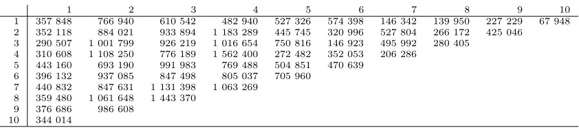
We analyze the data set from Taylor & Ashe (1983), even though the chain-ladder development

7 NUMERICAL STUDY 18

previous studies. The triangle of paid claims∇C is presented in Table 7.1.

1 2 3 4 5 6 7 8 9 10

1 357 848 766 940 610 542 482 940 527 326 574 398 146 342 139 950 227 229 67 948

2 352 118 884 021 933 894 1 183 289 445 745 320 996 527 804 266 172 425 046

3 290 507 1 001 799 926 219 1 016 654 750 816 146 923 495 992 280 405

4 310 608 1 108 250 776 189 1 562 400 272 482 352 053 206 286

5 443 160 693 190 991 983 769 488 504 851 470 639

6 396 132 937 085 847 498 805 037 705 960

7 440 832 847 631 1 131 398 1 063 269

8 359 480 1 061 648 1 443 370

9 376 686 986 608

10 344 014

Table 7.1:Observations of paid claims∇C from Taylor & Ashe (1983).

7.2. A comparison of the smoothing effects

In order to illustrate the smoothing effect of the model Figures 1 and 2 show the ln( ˆfj −1)

curves under the assumption of an ODP and a gamma distribution, respectively. Here ˆfj are the

estimated development factors before and after the smoothing. A sequence of deterministically

smoothed chain-ladder development factors has also been included in the figures for comparison.

It is difficult to compare the reparameterized GLM with the deterministic approach since there are

no rules of how to smooth the latter. As mentioned previously, the deterministic approach could

be varied in many different ways based on ad hoc decisions made by the actuary. However, in order

to construct a consistent and repeatable algorithm we have first applied a log-linear regression on

thetwolast chain-ladder development factors (this does of course not change the estimates, since

all we do is to draw the same line as before between the two factors). This would correspond to

r= 9. Secondly, we have applied a log-linear regression on thethreelast chain-ladder development

factors and created a new smoothed sequence using the first seven original factors and the three

new ones. This would correspond tor= 8. In this way we have proceeded through the sequences

until we included all the original factors in the log-linear regression and then created a smoothed

sequence which completely consists of new smoothed factors. This would correspond to r = 2.

Finally, we have fitted a straight line through origin, which would correspond to only one model

parameter and, hence,r= 1.

Note that the model r = 1 is of hardly any actual interest for reserving purposes, but we still

choose to include it here for completeness and illustration. In practice the first original factors are

7 N U M E R IC A L S T U D Y 1 9

1 2 3 4 5 6 7 8 9 −5 −4 −3 −2 −1 0 1 2 r=9

1 2 3 4 5 6 7 8 9 −5 −4 −3 −2 −1 0 1 2 r=8

1 2 3 4 5 6 7 8 9 −5 −4 −3 −2 −1 0 1 2 r=7

1 2 3 4 5 6 7 8 9 −5 −4 −3 −2 −1 0 1 2 r=6

1 2 3 4 5 6 7 8 9 −5 −4 −3 −2 −1 0 1 2 r=5

1 2 3 4 5 6 7 8 9 −5 −4 −3 −2 −1 0 1 2 r=4

1 2 3 4 5 6 7 8 9 −5 −4 −3 −2 −1 0 1 2 r=3

1 2 3 4 5 6 7 8 9 −5 −4 −3 −2 −1 0 1 2 r=2

1 2 3 4 5 6 7 8 9 −5 −4 −3 −2 −1 0 1 2 r=1

Figure 1: Theln( ˆfj−1)curves for the full GLM (− − −), the smoothed GLM (—) and the smoothed chain-ladder (· − ·) under the assumption of an ODP (p= 1) distribution.

7 N U M E R IC A L S T U D Y 2 0

1 2 3 4 5 6 7 8 9 −5 −4 −3 −2 −1 0 1 2 r=9

1 2 3 4 5 6 7 8 9 −5 −4 −3 −2 −1 0 1 2 r=8

1 2 3 4 5 6 7 8 9 −5 −4 −3 −2 −1 0 1 2 r=7

1 2 3 4 5 6 7 8 9 −5 −4 −3 −2 −1 0 1 2 r=6

1 2 3 4 5 6 7 8 9 −5 −4 −3 −2 −1 0 1 2 r=5

1 2 3 4 5 6 7 8 9 −5 −4 −3 −2 −1 0 1 2 r=4

1 2 3 4 5 6 7 8 9 −5 −4 −3 −2 −1 0 1 2 r=3

1 2 3 4 5 6 7 8 9 −5 −4 −3 −2 −1 0 1 2 r=2

1 2 3 4 5 6 7 8 9 −5 −4 −3 −2 −1 0 1 2 r=1

Figure 2: Theln( ˆfj−1) curves for the full GLM (− − −), the smoothed GLM (—) and the smoothed chain-ladder (· − ·) under the assumption of a gamma distribution

7 NUMERICAL STUDY 21

in a real application.

Recall that the factors for r = 9 under the assumption of an ODP in Figure 1 equal the pure

chain-ladder development factors, while the corresponding estimates under the assumption of a

gamma distribution in Figure 2 slightly differ. As can be seen, the reparameterized GLM yields a

smoother curve than the deterministic approach when it is used in the tail of the factor sequence.

Also note that the smoothed part of the curves is almost a straight line for large values ofr, just

as would be expected according to equation (3.13). For lower values ofrthe curves are convex in

comparison with the straight line obtained by the deterministic approach. The difference between

the assumptions of an ODP and a gamma distribution is the slope of the curve, which tends to

be lower for the latter one. However, for r= 4 the two curves coincide quite well. Note that the

reparameterized GLM yields a heavier tail than the deterministic approach. If the curve would be

extrapolated for a tail this might lead to an unrealictically large reserve according to the actuary’s

judgement.

A decision by eye would probably result in the use of one of the models r = 5,6 for the ODP

distribution andr= 5,6, or mayber= 7,8, for the gamma distribution. However, Figures 1 and

2 do not reveal how to choose between the two distributional assumptions. For the deterministic

approach we would choose the amount of smoothing corresponding to r = 5,6. However, this

approach does not yield maximum likelihood reserve estimates and we will instead focus on the

difference between the ODP and gamma assumptions for the reparameterized GLM.

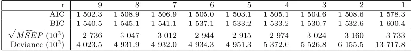
7.3. The model selection

AIC and BIC cannot be used as model selection criteria in (4.1) for the assumption of an ODP

distribution since we do not have a likelihood function due to the over-dispersion. However, the

square roots ofM SEPd in (4.6) are presented in Table 7.2. Recall that ˆφin (5.4) is used for the

resampling in the bootstrap procedure. We also present the deviance computed in the statistical

software used for the modeling (MATLAB); here it is defined as the sum of the squared deviance

residuals. As remarked in Section 4 the deviance does not penalize large models and, hence, it

7 NUMERICAL STUDY 22

AIC and BIC can be used for the assumption of a full gamma distribution with expected value

mij and varianceφm2ij, i.e.Cij ∼Γ

1

φ, φ mij

. Summing over then observations in∇C, which are assumed to be independent, yields

l(θˆ,φˆf ull_{) =} 1

ˆ φf ull

X

∇

−_mC_ˆij

ij −

log( ˆmij)

+X

∇

₁

ˆ φf ulllog

_C ij

ˆ φf ull

−log(Cij)−log Γ ₁

ˆ φf ull

.

The values of AIC and BIC are presented in Table 7.3 together with the square root of M SEPd

and the deviance.

As can be seen,M SEPd selects modelr= 5 orr= 9 for the assumption of an ODP distribution.

For the gamma assumption AIC andM SEPd select modelr= 9 orr= 5, while BIC selects model

r= 3 orr= 2. Hence, for the triangle under analysis AIC andM SEPd seem to be better selection

criteria than BIC, since modelr= 5 was one of the models chosen by eye in Section 7.2 too.

The number of parameterswhas large impact on the value of AIC in (4.4), since the log-likelihood

is quite constant for 5 ≤ r ≤ 8 for the triangle under analysis. This explains why AIC selects modelr= 9 orr= 5.

7.4. Reserve estimates and quantiles

The reserve estimates and bootstrap statistics under the assumption of an ODP and a gamma

distribution, respectively, are shown in detail in A. In Figure 3 we present the results graphically

in order to get an overview for different choices ofr. HereB= 10 000 iterations were used in the

bootstrap procedure.

As can be seen from (a), smoothing affects the reserve estimates in different ways for the

assump-r 9 8 7 6 5 4 3 2 1

p d

M SEP (103

) 3 039 3 222 3 247 3 114 3 000 3 051 3 234 3 659 4 921

Deviance (103

) 1 903.0 2 073.0 2 077.5 2 079.2 2 108.1 2 402.0 2 607.2 3 161.3 7 807.9

Table 7.2:The square root ofM SEPd in (4.6) and the deviance when an ODP distribution is assumed.

r 9 8 7 6 5 4 3 2 1

AIC 1 502.3 1 508.9 1 506.9 1 505.0 1 503.1 1 505.1 1 504.6 1 508.6 1 578.3

BIC 1 540.5 1 545.1 1 541.1 1 537.1 1 533.2 1 533.2 1 530.7 1 532.6 1 600.4

p d

M SEP (103

) 2 736 3 047 3 012 2 944 2 915 2 974 3 024 3 160 3 733

Deviance (103

) 4 023.5 4 931.9 4 932.0 4 934.3 4 951.3 5 372.0 5 526.8 6 155.5 13 717.8

7 N U M E R IC A L S T U D Y 2 3 1 2 3 4 5 6 7 8 9 1.7 1.8 1.9 2 2.1x 10

7 (a) Estimated reserve

1 2 3 4 5 6 7 8 9 1.7 1.8 1.9 2 2.1x 10

7 (b) Bootstrap mean

1 2 3 4 5 6 7 8 9 −3 −2.5 −2 −1.5 −1 −0.5 0 0.5x 10

5 (c) Bootstrap mean − Estimated reserve

1 2 3 4 5 6 7 8 9 2.5 3 3.5 4 4.5 5x 10

6 (d) Bootstrap standard deviation

1 2 3 4 5 6 7 8 9 2.5 3 3.5 4 4.5 5x 10

6 (e) sqrt(MSEP)

1 2 3 4 5 6 7 8 9 2.2 2.3 2.4 2.5 2.6 2.7 2.8 2.9x 10

7 (f) 95th percentile

Figure 3: Reserve estimates and bootstrap statistics for the assumption of an ODP and a gamma distribution, respectively. Here we use (− − −_{) for the ODP distribution}

7 NUMERICAL STUDY 24

tion of an ODP and a gamma distribution. For r = 4 the reserve estimates coincide, as was

already concluded in Section 7.2. The means of the bootstrap samples in (b) follow the reserve

estimates, with the latter ones being slightly larger since the difference in (c) is negative (but

ran-dom). Therefore,√M SEP in (e) is slightly larger than the standard deviation of the bootstrap samples in (d). The 95 percentiles in (f) mainly follow the shape of the reserve estimates, since

the standard deviations are relatively constant (except for the lowest values ofr).

In general, the first development factors of a sequence should be kept unsmoothed since they

are supposed to provide significant information regarding the data set. Hence, it is only relevant

to smooth the tail of the development factor sequence. However, Figure 3 shows that, for the

particular triangle under analysis, smoothing of the tail only has a minor effect on the results,

while the distributional assumption seems more important. To illustrate this, we investigate the

reserve estimate and the risk corresponding to the 95th percentile. Suppose that we start with the

chain-ladder method, i.e.r= 9 and the assumption of an ODP distribution, and, moreover, that

we decide to smooth the development factors using modelr= 5 in order to eliminate the shakiness

appearing in Figure 1. According to Tables A.1 and A.3 in the appendix we would then see a 1.5%

increase in the reserve estimate and a 0.8% increase in the 95th percentile. If we instead would

stick to r = 9, but assume a gamma distribution, we would see a 3.3% decrease in the reserve

estimate and a 4.3% decrease in the 95th percentile according to Tables A.2 and A.4.

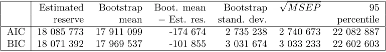
7.5. Implementing model selection in the bootstrap procedure

In this section, model selection is included in the bootstrap procedure, as described in Section 6,

for the assumption of a gamma distribution. The results are presented in Table 7.4. Recall that

ˆ

φf ull_{is always used for the calculation of AIC and BIC, but for the resampling of pseudo-triangles}

in the bootstrap procedure ˆφis used. Also recall that the first choice of model for AIC and BIC

wasr = 9 and r= 3, respectively, see Table 7.3. It is not possible to distinguish these results

Estimated Bootstrap Boot. mean Bootstrap √M SEP 95

reserve mean −Est. res. stand. dev. percentile

AIC 18 085 773 17 911 099 -174 674 2 735 238 2 740 673 22 082 887 BIC 18 071 392 17 969 537 -101 855 3 031 674 3 033 233 22 602 603

8 DISCUSSION 25

from the ones for r= 9 andr = 3, respectively, in Table A.4. Table 7.5 shows the frequency of

the selection of each model in the 10 000 iterations of the bootstrap, where it can be seen that

AIC strongly prefers high values ofr, while BIC does the opposite.

8. Discussion

In this paper, a model has been described which allows for smoothing of origin, development and

calendar year parameters. This smoothing model for the run-off pattern has some similarities

to the somewhat ad hoc log-linear smoothing of chain-ladder development factors which is often

used in practice. The suggested model is much simpler, but less flexible, than the GAM

frame-work presented in England & Verrall (2001) and the GLMM approach provided by Antonio &

Beirlant (2008). It can be used as a stochastic foundation for a claims reserving exercise

includ-ing smoothinclud-ing, model selection and bootstrappinclud-ing for either prediction errors or a full predictive

distribution.

While it is difficult to make any final conclusions from the single data set which has been analyzed

in this paper, it is interesting to note that the distributional assumption of the model had a

larger impact on the results than the smoothing effect. Hence, it seems important to first find an

appropriate model, which then possibly could be adjusted by smoothing of the model parameters.

The main weakness of a GLM with a log-link is that the model cannot be used for data sets

including negative increments when a full distribution is assumed. A future development would

be to use pure quasi-likelihood and the resulting estimating equations. In that case resampling of

residuals would be required for the bootstrap procedure.

r 9 8 7 6 5 4 3 2 1

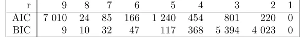
AIC 7 010 24 85 166 1 240 454 801 220 0

BIC 9 10 32 47 117 368 5 394 4 023 0

26

References

Antonio, K. & Beirlant, B., 2008. Issues in Claims Reserving and Credibility: a

Semi-parametric Approach with Mixed Models. The Journal of Risk and Insurance,75 (3), 643-676.

Barnett, G. & Zehnwirth, B., 2000. Best Estimates for Reserves. Proceedings of the Casualty

Actuarial Society,LXXXVII, 245-321.

Bj¨orkwall, S., H¨ossjer, O. & Ohlsson, E., 2009. Non-parametric and Parametric

Boot-strap Techniques for Age-to-Age Development Factor Methods in Stochastic Claims Reserving.

Scandinavian Actuarial Journal,4, 306-331.

England, P. & Verrall, R., 2001. A Flexible Framework for Stochastic Claims Reserving.

Proceedings of the Casualty Actuarial Society,LXXXVIII, 1-38.

England, P. & Verrall, R., 2002. Stochastic Claims Reserving in General Insurance. British

Actuarial Journal,8(3), 443-518.

Kremer, E., 1982. IBNR Claims and the Two Way Model of ANOVA.Scandinavian Actuarial

Journal, 47-55.

Liang, K.-Y. & Zeger, S., 1986. Longitudinal Data Analysis Using Generalized Linear Models.

Biometrika,73, 13-22.

Miller, A., 2002. Subset Selection in Regression. Chapman and Hall, Boca Raton.

Pan, W., 2001. Akaike’s Information Criterion in Generalized Estimating Equations. Biometrics,

57(1), 120-125.

Pan, W. & Le, C. T., 2001. Bootstrap Model Selection in Generalized Linear Models. Journal

of Agricultural, Biological, and Environmental Statistics,6(1), 49-61.

Renshaw, A. & Verrall, R., 1998. A Stochastic Model Underlying the Chain Ladder Technique.

27

Sherman, R., 1984. Extrapolating, Smoothing and Interpolating Development Factors.

Proceed-ings of the Casualty Actuarial Society,LXXI, 122-192.

Wedderburn, R. W. M., 1974. Quasi-Likelihood Functions, Generalized Linear Models, and

the Gauss-Newton Method. Biometrika,61, 439-447.

Verrall, R., 1989. A State Space Representation of the Chain Ladder Linear Model. Journal of

the Institute of Actuaries,116, 589-609.

Verrall, R., 1996. Claims Reserving and Generalized Additive Models. Insurance: Mathematics

and Economics,19, 31-43.

Verrall, R., 2007. Obtaining Predictive Distributions for Reserves which Incorporate Expert

Opinion. Variance,1, 53-80.

Verrall, R. & England, P., 2005. Incorporating Expert Opinion into a Stochastic Model for

the Chain-ladder Technique. Insurance: Mathematics and Economics,37, 355-370.

Wright, T., 1990. A Stochastic Method for Claims Reserving in General Insurance. Journal of

the Institute of Actuaries,117, 677-731.

W¨utrich, M. & Merz, M., 2008. Stochastic Claims Reserving Methods in Insurance. John

Wiley & Sons Ltd.

Zehnwirth, B., 1985. ICRFS Version 4 Manual and Users Guide. Benhar Nominees Pty. Ltd.,

Tumurra, NSW, Australia.

Zehnwirth, B., 1989. Regression methods - Applications. Conference paper, 1989 Casualty Loss

Reserve Seminar. Available online at:

28

SUSANNA BJ ¨ORKWALL

Department of Mathematics,

Division of Mathematical Statistics

SE-106 91 Stockholm University

A APPENDIX 29

A. Appendix

Year r= 9 r= 8 r= 7 r= 6 r= 5 r= 4 r= 3 r= 2 r= 1

2 94 634 240,187 221 536 230 156 202 906 142 453 178 698 234 891 397 438

3 469 511 490 001 468 650 481 624 435 577 322 911 394 173 505 214 826 224

4 709 638 769 423 767 511 778 890 725 379 571 929 677 310 844 415 1 330 160

5 984 889 1 039 712 1 029 537 1 029 175 992 396 840 830 961 998 1 162 612 1 755 176

6 1 419 459 1 477 137 1 466 432 1 473 134 1 483 356 1 373 765 1 508 001 1 756 918 2 521 484

7 2 177 641 2 241 521 2 229 665 2 237 087 2 208 130 2 310 842 2 399 913 2 667 064 3 585 818

8 3 920 301 3 996 865 3 982 655 3 991 552 3 956 845 3 864 518 3 655 170 3 776 692 4 609 461

9 4 278 972 4 342 643 4 330 826 4 338 225 4 309 362 4 232 583 4 278 865 3 735 382 3 778 936

10 4 625 811 4 681 894 4 671 485 4 678 001 4 652 579 4 584 950 4 625 716 4 690 754 2 155 908

Total 18 680 856 19 279 383 19 168 297 19 237 844 18 966 529 18 244 781 18 679 843 19 373 942 20 960 607

Table A.1:The estimated reserves under the assumption of an ODP distribution.

Year r= 9 r= 8 r= 7 r= 6 r= 5 r= 4 r= 3 r= 2 r= 1

2 93 316 202 152 203 511 207 892 199 638 172 114 184 757 211 549 309 558

3 446 505 408 480 409 958 416 799 404 635 351 964 376 550 429 348 639 118

4 611 145 629 353 629 086 632 612 618 547 574 367 611 511 688 582 1 018 712

5 992 023 1 008 479 1 008 970 1 003 960 996 081 934 022 967 584 1 073 045 1 415 607

6 1 453 085 1 470 922 1 471 480 1 473 661 1 497 337 1 481 516 1 511 006 1 616 061 2 080 145

7 2 186 161 2 209 807 2 210 383 2 212 695 2 206 567 2 416 362 2 386 357 2 497 200 3 015 061

8 3 665 066 3 687 154 3 687 803 3 689 857 3 684 059 3 651 627 3 402 313 3 351 061 3 906 657

9 4 122 398 4 139 309 4 139 832 4 141 344 4 136 502 4 107 371 4 118 985 3 557 488 3 149 813

10 4 516 073 4 532 001 4 532 447 4 532 966 4 528 998 4 502 114 4 512 328 4 524 778 1 755 546

Total 18 085 773 18 287 657 18 293 470 18 311 784 18 272 364 18 191 456 18 071 392 17 949 111 17 290 218

Table A.2: The estimated reserves under the assumption of a gamma distribution.

Estimated Bootstrap Boot. mean Bootstrap √M SEP 95

r reserve mean −Est. res. stand. dev. percentile

9 18 680 856 18 502 852 -178 004 3 034 174 3 039 240 23 187 718

8 19 279 383 19 055 285 -224 098 3 214 046 3 221 689 24 027 278

7 19 168 297 18 889 878 -278 419 3 235 449 3 247 245 23 830 275

6 19 237 844 19 058 883 -178 961 3 108 771 3 113 762 23 825 274

5 18 966 529 18 749 895 -216 634 2 992 653 3 000 334 23 365 377

4 18 244 781 18 089 415 -155 366 3 047 533 3 051 339 22 742 333

3 18 679 843 18 457 164 -222 679 3 226 904 3 234 417 23 442 951

2 19 373 942 19 159 588 -214 354 3 652 746 3 658 848 24 738 289

1 20 960 607 20 727 316 -233 291 4 915 800 4 921 087 28 065 538

Table A.3:Bootstrap results for the total under the assumption of an ODP distribution.

Estimated Bootstrap Boot. mean Bootstrap √M SEP 95

r reserve mean −Est. res. stand. dev. percentile

9 18 085 773 17 943 796 -141 977 2 732 628 2 736 177 22 233 262

8 18 287 657 18 099 941 -187 716 3 041 109 3 046 746 22 767 497

7 18 293 470 18 109 290 -184 180 3 006 144 3 011 631 22 706 271

6 18 311 784 18 122 332 -189 452 2 938 433 2 944 387 22 707 132

5 18 272 364 18 073 957 -198 407 2 908 233 2 914 848 22 545 380

4 18 191 456 18 049 088 -142 368 2 970 365 2 973 626 22 612 284

3 18 071 392 17 885 372 -186 020 3 018 708 3 024 283 22 558 091

2 17 949 111 17 791 615 -157 496 3 156 046 3 159 815 22 611 167

1 17 290 218 17 086 896 -203 322 3 727 575 3 732 930 22 702 370