The Added Value from a General Equilibrium Analyses of Increased Efficiency in Household Energy Use

D

E

U

S

G

THE ADDED VALUE FROM A GENERAL EQUILIBRIUM ANALYSES

OF INCREASED EFFICIENCY IN HOUSEHOLD ENERGY USE

B

PATRIZIO LECCA, PETER MCGREGOR,

J. KIM SWALES, KAREN TURNER

NO. 13-08

S

TRATHCLYDE

1

The added value from a general equilibrium analyses of increased efficiency

in household energy use

Patrizio Lecca1,a, Peter G. McGregor1, J. Kim Swales1 and Karen Turner2

1. Fraser of Allander Institute and Department of Economics, University of Strathclyde

2. Department of Accounting, Economics and Finance, School of Management and

Languages, Heriot Watt University.

a. Corresponding author: E-mail:patrizio.lecca@strath.ac.uk;

May 2013

Acknowledgments

The authors gratefully acknowledge the financial support of the ESRC through a First Grants

project (ESRC ref: RES-061-25-0010), the EPSRC Highly Distributed Energy Futures

2

Value-added from a general equilibrium analyses of increased efficiency in

household energy use

Abstract

The aim of the paper is to identify the added value from using general equilibrium techniques

to consider the economy-wide impacts of increased efficiency in household energy use. We

take as an illustrative case study the effect of a 5% improvement in household energy

efficiency on the UK economy. This impact is measured through simulations that use models

that have increasing degrees of endogeneity but are calibrated on a common data set. That is

to say, we calculate rebound effects for models that progress from the most basic partial

equilibrium approach to a fully specified general equilibrium treatment. The size of the

rebound effect on total energy use depends upon: the elasticity of substitution of energy in

household consumption; the energy intensity of the different elements of household

consumption demand; and the impact of changes in income, economic activity and relative

prices. A general equilibrium model is required to capture these final three impacts.

Keywords: Energy efficiency; indirect rebound effects; economy-wide rebound effects;

household energy consumption; CGE models.

3

1. Introduction

Economy-wide rebound effects resulting from energy efficiency improvements in production

have been extensively investigated. This analysis has often used a computable general

equilibrium (CGE) modelling framework (see Dimitropoulos, 2007; Sorrel, 2007; and Turner

2013for a review). However, very few studies attempt to measure the economy-wide impacts

of increased energy efficiency in the household sector. Following the work of Khazzoom

(1980, 1987) there have been a numbers of partial equilibrium studies (Dubin et al. 1986;

Frondel et al. 2008; Greene et al. 1999; Klein, 1985 and 1987; Nadel, 1993; Schwartz and

Taylor, 1995; West, 2004). Further, Greening et al. (2000) gives a detailed and extensive

summary of the extent of rebound on household consumption for several types of energy

services. This literature assumes that there are no changes in prices or nominal incomes

following the efficiency improvement and that impacts are limited to the direct market for

household energy use. This approach permits consideration of the direct rebound effect only.

To our knowledge, Dufournaud et al. (1994) is the only study that investigates economy-wide

rebound effects from increased energy efficiency in the household sector. It examines the

impacts of increasing efficiency in domestic wood stoves in Sudan. Druckman et al. (2011)

and Freire-Gonzalez (2011) use a fixed price input-output model to consider indirect rebound

effects resulting from household income freed up by energy efficiency improvements and

spent on non-energy commodities. However, we consider their work an extension of partial

equilibrium analysis in that they fail to consider endogenous prices, incomes or factor supply

effects.

The aim of the present paper is to identify the added value from using general equilibrium

4

use. We take as an illustrative case study the impact of a 5% improvement in household

energy efficiency. This impact is measured through simulations that use models that have

increasing degrees of endogeneity but are calibrated on a common UK data set. That is to say,

we calculate rebound effects for models that progress from the most basic partial equilibrium

approach to a fully specified general equilibrium treatment.

The reminder of the paper is structured as follows. In Section 2 we define rebound effects in

household and total energy use and show how these are calculated. In Section 3 we estimate a

key parameter in the determination of the rebound effect, the elasticity of substitution between

energy and non-energy commodities in household consumption. Section 4 considers the

partial equilibrium household and total energy use rebound values and investigates the

relationship between the two. Section 5 introduces the AMOS computable general

equilibrium modelling framework. In Section 6, this model is used in general equilibrium

rebound simulations. In Section 7 we comment on the range of rebound values and identify

the value-added from adopting a general equilibrium approach and Section 8 is a short

conclusion.

2 Rebound Effects

To begin, it is useful to specify what we mean by an increase in energy efficiency. We

categorise an increase in household energy efficiency as being a change in household

“technology” such that the energy services per unit of physical energy is increased. An

alternative way of expressing this is that the energy value in efficiency units has risen.1 This

implies that the original level of household utility can be achieved through the consumption of

5

the original levels of other household goods and services, but a lower input of energy

consumption.2

We define the rebound effect generated by an increase in energy efficiency as a measure of

the difference between the proportionate change in the actual energy use and the proportionate

change in energy efficiency. This difference is primarily driven by the fact that, ceteris

paribus, an increase in the efficiency in a particular energy use reduces the price of energy in

that use, measured in efficiency units. This reduction then leads consumers to substitute

energy, in efficiency units, for other goods and services.

This distinction between energy quantity and price measured in natural and efficiency units is

important in explaining how the rebound effect operates. However, in the present paper,

unless we explicitly state otherwise energy is being measured in natural units. The fall in the

price of energy, measured in efficiency units, implies that proportionate change in energy use

is typically less than the proportionate change in energy efficiency. This is the rebound effect.

Moreover, in principle, energy use can actually rise in response to an improvement in energy

efficiency, if its use is sufficiently price sensitive. This is known as backfire (Khazzoom,

1980 and 1987).

In this paper we investigate the impact of an improvement in the efficiency of energy use in

household consumption. In this case, for a proportionate improvement in household energy

use of γ, rebound in the household consumption of energy, RC, is measured as:

1 C 100

C

E R

γ

 

= +_{ }⋅

 



(1)

2

6

where E_C is the proportionate change in energy use in household consumption.

In interpreting equation (1) it is important to be mindful of the sign of the proportionate

change in energy use,E_C. If in the case we consider, the 5% efficiency improvement leads to

a corresponding 5% reduction in energy use in consumption, the rebound value RC would be

zero; there would be no rebound. However, if the fall in energy use were less than 5%, then

there would be a positive rebound, which increases as the reduction in energy use takes

smaller absolute values. Rebound is 100% if the use of energy is unaffected by the increased

efficiency: if the impact on energy use is positive, then rebound is greater than 100% and this

is known as backfire.

We are also interested to the economy-wide rebound within the target economy3 of household

energy efficiency improvements on total energy use; that is to say, energy used both in

consumption and production. The total rebound formulation used in this case, RT, is given as:

1 T 100

T E R αγ   = +_{ }⋅    (2)

where α is the initial share of household energy consumption in total energy use. The term

T

E

αγ



can be expressed as:

C P C

T T P

C C C

E E E

E E E

E E E

αγ γ γ γ γ

∆ + ∆

∆ ∆

= = =  +



(3)

where Δ represents absolute change and the P subscript indicates production. Substituting

equation (3) into equation (2) and using equation (1) gives:

3 _{Our interest here is limited to the macro level rebound effect within the target economy. That is to say we are}

7

100 P

T C

C

E R R

E

γ ∆

= + ⋅ (4)

This shows that the total rebound will be greater than the consumption rebound if the energy

use in production increases as a result of increases in efficiency in energy use in consumption.

If, on the other hand, energy use falls in production, total rebound is lower than consumption

rebound.

3. Data and elasticity of substitution of energy use in consumption

In this paper we identify the additional precision achieved through moving from a partial to a

general equilibrium analysis of the rebound effects. We consider the specific case of energy

efficiency improvements in household consumption. 4 We quantify the rebound effect through

simulation using a given data set which provides common structural characteristics across all

the models. Specifically we use a specially constructed UK symmetric industry-by-industry

Input-Output table based on the published 2004 UK Supply and Use Tables.5 Import data in

input-output format were provided by colleagues at the Stockholm Environment Institute. The

input-output accounts are aggregated to identify 21 economic activities

(commodities/sectors). Table 1 gives the sectoral disaggregation, separately identifying four

energy sectors; coal, oil, gas and electricity.

In Table 2, we report the energy input requirement for each of the production sectors and the

energy-output multiplier effects expressed in monetary terms. That is to say, for each sector

we measure the direct and indirect increase in the value of output in energy industries

4

We are increasing energy efficiency in all energy use: coal, oil, gas and electricity.

8

generated by a unit increase in the final demand for that sector. The energy requirements are

represented by the appropriate direct input-output coefficients (the A matrix) while the

energy-output multipliers correspond to the Type I Leontief inverse, [1-A]-1. To calibrate the

Computable General Equilibrium model, the conventional Input-Output accounts are

augmented with all other transfer payments to form the 2004 UK Social Accounting Matrix.6

In all the analysis we have a single initial vector of household consumption given in UK 2004

Input-Output accounts.

A key parameter that drives rebound analysis is the elasticity of substitution between

aggregate energy and non-energy goods and services in the household’s utility function. In

each of the models we use, household utility, C, in any period is given by:

1 1 ₁

(1 )

E E

C C

C E NE

ε

ε ε _ε

ε ε

δ γ δ

− − − ₋

 

=_ + − _

 

(5)

Where, NEC is the consumption of non-energy commodities, ε is the elasticity of substitution

between energy and non-energy commodities in consumption and δE∈(0,1) is the share

parameter.

We estimate the value of the elasticity of substitution using UK household consumption data

from 1989 to 2008.7 Details about the estimation procedure are reported in Appendix 1 and

Lecca et al (2011a). As expected, consumer demand is more sensitive to prices over the long

run than the short run: the short- and long-run elasticities of substitution are estimated as 0.35

and 0.61 respectively. The estimation uses the conventional generalized maximum entropy

6 _{For more information on Input-Output accounts and Social Accounting Matrices see Miller and Blaire (2009).} 7

9

(GME) method (Golan et al. 1996). This is a widely used technique for generating parameter

estimates for CGE models, though for comparative purposes OLS estimates are also reported

in the Appendix 1. Our estimated elasticity values are broadly in line with previous empirical

evidence for the UK households (e.g. Baker and Blundell, 1991 and Baker et al. 1989).

We have estimated the substitution elasticities by observing the reaction of household energy

consumption to changes in energy price. However, the question arises as to whether the same

substitution elasticities are appropriate for changes in the use of energy where efficiency

improvements have reduced the price of energy, measured in efficiency units? The answer

might lie in the nature of the efficiency improvement. We see no reason not to use the

long-run elasticity of substitution where long-long-run simulations are performed. However, for

short-run simulations we will argue that it in some circumstances might be appropriate to use the

long-run elasticity value.

The short-run adjustment in household consumption of energy in response to a change in

energy prices might be lower than the long-run value for two different reasons. First, there

might be a degree of inertia in the consumption response: it might take time before the

consumer is aware that the energy price has changed and he or she might exhibit a degree of

lethargy in making the appropriate adjustment in consumption. However, a second reason

might be that a full adjustment to the new energy price requires an investment in consumer

durable goods, which only occurs in the long run.

For example, imagine that the price of gasoline falls. In the short run consumers will make

more and longer trips in their existing cars. However, in the long run, when a new car is

purchased, consumers might also increase the engine capacity, and therefore fuel

10

the need to make complementary adjustments in consumer durables to fully exploit the

change in price.

These arguments are relevant for analysing the impact of an improvement in household

energy efficiency. If energy efficency is not embodied in capital equipment, it should operate

in a way analogous to a price change. For example, imagine that chemical additives to

gasolene increases the miles per gallon achieved by all cars by the same proportionate extent.

In this case we should use the different short- and long-run elasticities for analysing the

corresponding time periods. That is to say, the short-run adjustment should have motorists

more frequently and extensively using their cars, whilst a fuller adjustment is possible in the

long run where the type of car, size of engine etc. might change as a result of lower effective

gasolene costs.

However, if the energy efficiency improvement is embeddded in the design of a consumer

durable, then the efficiency improvement is not experienced untill the consumer purchases a

new vintage. For example, the improvement in energy efficiency might be delivered through a

new car engine design. This implies that the efficiency increase is not experienced untill the

new engine is purchased. However, it is likely that this will be coincident with decisions taken

over the size of the car, car engine etc. Therefore these are decisions where the long-run value

of the elasticity of substitution is relevant. This is so even in the short run, where the rest of

the economy has not fully adjusted to the implied price and income changes flowing from the

energy efficiency improvement.

11

In the partial equilibrium analysis applied here, we assume that the prices of all commodities

and services, including energy prices, are fixed and that there is no change in household

nominal income. This is the impact that would be appropriate for analysing the decision by a

single household to introduce improvements in energy efficiency. However, although we

focus on an improvement in energy efficiency in consumption, we are also interested in the

subsequent impact on energy use in production too. This can be achieved, in this case, whilst

still maintaining the partial equilibrium assumptions of fixed prices and household income,

through the application of conventional Type I Input-Output analysis.

4.1 Household energy use

To determine the level of rebound in household energy use, first we need to derive the

elasticity of demand, η, from the elasticity of substitution, ε. This is given as (Gørtz, 1977):

( 1)

η ε ε= − − λ (6)

where λ is the share of energy in household expenditure. From the UK 2004 Input Output

accounts, 3% of household consumption is spent on energy so that λ = 0.03. In Section 3 we

report the values for the short- and long-run elasticities of substitution as 0.35 and 0.61

respectively. Therefore from equation (6), the short- and long-run energy price elasticities of

demand are given as 0.369 and 0.622.

With no change in the price of energy, a proportionate increase in efficiency in household

energy consumption, γ, generates an equal proportionate reduction in the price of energy to

consumers, measured in efficiency units. If the elasticity of demand for energy is η, where η

takes a positive sign, the proportionate change in consumer energy demand, again measured

in efficiency units, E_CF, is given as:

F C

12

The proportionate change in consumer energy use, measured in natural units, is the

proportionate change in efficiency units, minus the change in efficiency:

( 1)

C

E =ηγ γ− = η− γ (8)

where η ≥0and EC γ 0 η

∂

= > ∂



. If energy demand is completely price inelastic, so that η=0,

household energy use falls by the full proportionate amount, γ. On the other hand where price

elasticity equals one, energy use is unchanged. If demand is price elastic, so that η > 1,

household energy use increases as a result of improvements in household energy efficiency.

Substituting expressions (6) and (8) into equation (1) produces:

100 100( ( 1) )

C

R = η= ε− −ε λ (9)

Using the short- and long-run demand elasticities produces the short- and long-run rebound

values of 36.9% and 62.2%.8 These values are entered in the top row of Table 3.

Equation (9) calculates what is conventionally known as the direct rebound. These figures lie

within the range of available US and European estimates for specific household energy uses

(see e.g. Greening et al., 2000 and Freire-Gonzales, 2010). A comprehensive review of empirical

estimates of direct rebound effects is provided by Sorrell et al. (2009).

4.2 Total energy use

In the analysis reported in Section 4.1, the improvement in energy efficiency operates in a

manner that is observationally equivalent to a change in the representative household’s tastes,

with fixed nominal income and prices. That is to say, the improvement in energy efficiency is

8

13

reflected solely in consumption shifting.9 With rebound values less than 100%, as reported

here, this implies a fall in consumption expenditure on energy and an increase in the

expenditure on all other goods and services.10

We can retain the partial equilibrium assumptions of fixed prices and household income but

incorporate the impact on total energy use by adopting a Type I Input-Output analysis (Miller

and Blair, 2009). In this approach, the impact on energy use in both household consumption

and industrial production is identified and the relevant total rebound measure, as expressed in

equation (2), can be calculated. This captures the notion of energy being embodied in

consumption goods or services, in the form of the energy required, directly or indirectly, in

the production of these goods and services (Miller and Blaire, 2009, and Sorrel, 2009).

We introduce a shock in the Input-Output system by reducing household final consumption

expenditure on (both UK and imported) energy (coal, oil, gas and electricity) to reflect the

reduced energy requirement when efficiency in household energy use rises in line with the

analysis in the previous section. We simultaneously increase household spending on other

(non-energy) goods and services, using the distribution of initial expenditure on (domestic

and imported) non-energy goods and services. This distribution is given in the Input-Output

accounts. This method shares some characteristics with Freire-Gonzalez (2011): it extends

Druckman et al. (2011) by incorporating the impact on indirect rebound from the reduction in

energy use embodied in the reduction in energy supply itself.

The change in household consumption expenditure on energy, ΔEC, is matched by an equal

and opposite change in non-energy household expenditure, ΔNEC, and is given as:

9

An increase in energy efficiency with fixed prices and nominal income does mean that household utility will rise. The implications of this are dealt with in more detail in Section 6.2.

10 _{However, if backfire occurs, so that rebound is greater than 100%, household expenditure on energy will rise}

14

1 100

C

C C T

R

E NE X  λγ

∆ = −∆ = _ − _

  (10)

where XT is total household expenditure. Using Type I Input-Output multipliers, the change in

total energy use, ΔET, equals:

(1 E) E

T C E C N

E E m NE m

∆ = ∆ + + ∆ (11)

where E E

m and E

N

m are respectively the amounts of energy used, directly or indirectly, in the

production of one unit of energy and one unit of non-energy household consumption.

Household energy use can be expressed either as the share, λ, of the total household

expenditure or a share, α, of the total energy use. Using this result produces:

T

X E λ

α

= (12)

Using equations (10), (11) and (12) produces:

1 (1 )

100

E E

C

T E N

R

E =αγ_ − _ +m −m

 

 ₍₁₃₎

Using the notation E E E

E N

m m m

∆ = − and substituting equation (13) into equation (2) gives:

( 100) E

T C C

R =R + R − ∆m (14)

Equation (14) expresses the total partial equilibrium rebound as a function of the rebound

value in the household consumption of energy, RC, and the difference between the embodied

energy in the production of energy and non-energy goods and services, ΔmE. We expect the

production of energy to be relatively energy intensive, so that E E

E N

m >m , and therefore that

ΔmE

15

equation (14), this implies that the relationship between the partial equilibrium household

consumption rebound and total rebound is represented in Figure 2.11

Consider first the situation where the household consumption rebound is 100%. This means

that there is no change in the household use of energy as a result of the efficiency

improvement. There is therefore similarly no change in production: RT = RC = 100%. If

household consumption rebound is greater than 100%, so that backfire occurs in household

consumption of energy, then consumers spend a greater share of their income on energy after

the efficiency improvement. Because the production of energy is relatively energy intensive,

this means that the energy used in production increases and the total rebound value will be

greater than the household rebound: RT > RC. On the other hand, if rebound is less than 100%,

household consumption switches to non-energy commodities. This implies that the total

energy use rebound will be less than the household consumption rebound, as energy use in

production falls. If 100

1 E

C E

m R

m

 ∆ 

<  _{+ ∆} 

  , then the total rebound is actually negative. That is to

say, the proportionate reduction in total energy use, measured as a percentage of the initial

household energy use, is greater than the efficiency improvement. Where the household

consumption rebound is zero, the total rebound equals -100ΔmE.

We can quantify the partial equilibrium total rebound generated by the consumption

expenditure shifting associated with the improvement in household energy efficiency. For the

36.90% household consumption rebound value estimated using the short-run elasticity of

substitution, the proportionate reduction in household consumer expenditure on energy,E_C,

equals 3.16%. Where γ = 5% and α = 0.344, this corresponds to a 109355 TJ reduction in

11

16

household energy use and to a £752.57 million reallocation in UK household consumption

across the seventeen non-energy consumption sectors, in line with the initial distribution of

expenditure (domestic and imported) in those sectors. The result is a fall in total energy

demand of £1002 (137363 TJ) which corresponds to 1.44% of total UK energy use (across

households and producers), so that ĖT = - 1.44% _{. This produces a total rebound value (}RT)

of 15.96%. Given that the household consumption rebound (RC) is positive, at 36.9%, the

indirect component of the rebound effect is negative with a value of 20.94%. 12

Given that energy is disaggregated into four separate sectors in the Input-Output accounts, we

can calculate a separate total rebound value for each energy type. In this simulation, we

impose the same energy efficiency improvement across all energy sectors and the same

household consumption demand elasticity. Therefore all the energy sectors will have the same

short-run household consumption rebound value of 36.9%. However, the total rebound effects

vary dramatically.

The value for the total rebound for coal is negative, at -53.49%. As a result of the 5%

improvement in efficiency in the use of all energy types in household consumption, the total

demand for coal will fall by 1.01%. The classic rebound effect limits the improvement in

energy efficiency: however in this case the efficiency impact is magnified. This is because the

use of coal in household consumption is low, but its use as an intermediate input into energy

(primarily electricity) production is high. Therefore the positive rebound effects in household

consumption are swamped by negative rebound effects from the reduced demand for coal in

production, particularly as electricity output falls.

12_{From the figures given in Table 3 the value of the differential intermediate energy multiplier, Δm}E_{, as used in}

17

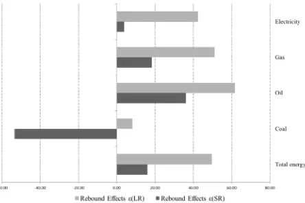
For the other three energy sectors (gas, electricity and oil), the total short-run rebound values

are all positive, with values of 18.30%, 3.81% and 36.01% respectively. The rebound value

for electricity is below, and the values for gas and oil are above, the value for the combined

energy sector.

Where the estimated long-run demand elasticity is used in the rebound calculations, there is a

larger household consumption rebound value. This implies a smaller reallocation of

household expenditure in favour of non-energy goods and services. In this case, E_Cindicates

a 0.87% fall in expenditure on energy, a reduction of 65509 TJ which equates to £450.9

million to be reallocated to non-energy household consumption. The total energy rebound, RT,

is 49.66%, with the impact of indirect expenditures (RT-RC) being to reduce the rebound by

12.54 percentage points. The rebound effect for the four individual energy sectors is now

positive for all energy-types: 8.05% for coal, 51.06% for gas, 42.38% for electricity and

61.67% for oil. The ranking of the sectors remains the same, both relative to each other and

also with the combined energy use value. Specifically, the total rebound values for gas and oil

use are slightly higher than the combined energy household consumption values, electricity

and coal are lower.

Generally, there is an expectation that the total rebound will be bigger than the household

consumption value. However, this will not typically be the case. Energy production is usually

more (directly and indirectly) energy-intensive than non-energy production. If rebound is less

than 100%, the reallocation of the budget reduces the household expenditure on energy and

increases it on non-energy commodities and services. In this case, the indirect component of

18

5. General equilibrium rebound effects – endogenous prices and incomes

The analysis in Section 4 holds prices and nominal household income fixed. However, as the

demand for goods and services varies, if there are any constraints on supply, prices will also

change. This will affect sectoral revenues, the returns to factors of production and also

household incomes. In the analysis in this section we allow prices and incomes to vary in

determining the rebound effect. These effects are captured through the use of Computable

General Equilibrium (CGE) modelling.

5.1 The UKENVI CGE Model

To identify the general equilibrium impacts, we use a variant of the UKENVI CGE modelling

framework. This is an energy-economy-environment version of the basic AMOS CGE

framework, calibrated on UK data (Allan et al. 2007; Harrigan et al. 1991 and Turner,

2009).13 However, in contrast to previous applications of UKENVI, in this version

consumption and investment decisions reflect inter-temporal optimization with perfect

foresight (Lecca et al. 2010).

We identify the same twenty one economic activities (commodities/sectors) as considered in

the input-output analysis in Section 4. There are three domestic transactor groups:

13

19

government, households and firms. In this application government expenditure is fixed in real

terms. Households optimise their lifetime utility, which is a function of consumptionC_t

taking the following form:

σ ρ σ − −       + = ∞ − =

∑

1 1 1 0 t t t C U (15)

where Ct is the consumption at time period t, σ andρ are respectively the constant elasticity

of marginal utility and the constant rate of time preference. The intra-temporal consumption

bundle, Ct, is defined, as in the partial equilibrium simulations, as a CES combination of

energy and non-energy composites, as given in equation (5) in Section 2. In our empirical

analysis we consider consumption of both domestic and imported energy and non-energy

goods, where imports are determined through an Armington link and are therefore

relative-price sensitive (Armington, 1969).

The consumption structure is shown in Figure 2. Total consumption is divided in energy and

non-energy goods and services. The consumption of energy is then a CES combination of two

composites: gas and electricity, and oil and coal. The production structure as imposed in each

sector is shown in Figure 3. In each sector the input decision involves a hierarchy of CES

relationships between inputs of intermediate goods, labour and capital.

The path of investment is obtained by maximizing the present value of the firm’s cash flow

given by profit, π_t, less private investment expenditure, It, subject to the presence of

adjustment cost g

( )

Max

(

)

[

(

( )

)

]

∑

t I g

r π ω subject to Kt =It −δKt

20

The solution of the dynamic problem gives us the law of motion of the shadow price of

capital,λ_t, and the time path of investment related to the tax-adjusted Tobin’s q.

The UK labour force is assumed to be fixed, with the real wage determined through a wage

function that embodies the econometrically derived specification given in Layard et al.

(1991):

[ ]

where w, cpi and u are the nominal wage after tax, the consumer price index and the

unemployment rate respectively, and c is a parameter which is calibrated so as to replicate

equilibrium in the base year.

In each sector, exports are determined by a standard export demand function.

In our second scenario, the increased energy efficiency in household consumption is directly

reflected in the real wage determination given in equation (17). This involves modifying the

cpi so that the price of energy services is expressed in efficiency units. In the conventional

approach, cpi is simplyas a function of the price of commodities:

(18)

where pNE is the price of non-energy goods and services and pE is the price of energy

services, both measured in natural units. If τ is used to identify an efficiency unit of energy,

with a γ percentage change in in energy efficiency in household consumption, we can

incorporate the efficiency change in the wage bargaining process by simply adjusting the cpi

by measuring the price of energy in efficiency units. This goes as follows:

E E p p p < + = γ τ

1 for γ >0 (19)

) , (pNE pE

cpi

21

So that

) ,

( _τ

τ cpi p p

cpi = _NE (20)

where pτ is the price of energy measured in efficiency units. This means that with constant

energy prices in natural units,p_E, an improvement in energy efficiency reduces the price of

energy in terms of efficiency units, p_τ. In this scenario, this reduces the cpi and has a direct

effect on the nominal wage rate.

5.2. Calibration and key model parameters

The model calibration process assumes the economy to be initially in steady state equilibrium.

The key dataset is the UK Social Accounting Matrix, which incorporates the 2004 Input

Output table used in Section 4. However, we need also to impose a number of important

behavioural parameters. First, as in all the partial equilibrium simulations, we adopt the

estimated values for the short- and long-run elasticity of substitution between energy and

non-energy goods and services in household consumption given in Section 3. Trade elasticities are

set equal to 2 (Gibson, 1990) and production elasticities equal to 0.3 (Harris, 1989). The

interest rate (faced by producers, consumers and investors) is set to 0.04, the rate of

depreciation to 0.15 and with constant elasticity of marginal utility equal to 1.2 (Evans, 2005).

5.3 Simulation strategy

As in the partial equilibrium simulations, we introduce a costless and permanent step

efficiency increase of 5% in energy use in household consumption. We report results for two

22

impacts for some simulations. The short-run corresponds to the first period of the simulation,

where the initial capacity constraints are present. That is to say, in this time interval the

capital stock is fixed, both in its total and its sectoral composition, at the base period values.

However, from period two, capital stock adjusts through investment and depreciation. In the

long run, the state variables of the model are subject to transversality conditions, so as to

obtain a new steady-state.

As discussed in Section 4, the appropriate value to use for the elasticity of substitution

between energy and non-energy commodities in household consumption is not

straightforward. When the analysis applies to the long run, we always use the long-run

elasticity of substitution. However, in the short run, as argued in Section 3, we perform

simulations using both the short-run and long-run substitution elasticities.

6. General Equilibrium rebound results

Table 4 shows the impact of the improved household energy efficiency on key

macroeconomic variables using the conventional perfect foresight AMOS model. We label

this Scenario 1. We report the results as percentage changes from the base year values. The

short-run figures are given for both the short- and long-run estimated values of the elasticity

of substitution between energy and non-energy commodities in household consumption.

Recall, that we argue there that the long-run elasticity values might be more appropriate, even

in short-run simulations, if energy efficiency is embodied in the design of consumer durables.

In Scenario 2, the model is adjusted, as shown in in equation (19) and (20) in Section 5.1, so

that the cpi incorporates the price of energy in efficiency, rather than natural, units. In Table

23

6.1 Scenario 1: The standard model

The simulation results using the standard AMOS model are given in Table 4. In the short run

in Scenario 1, employing the short-run elasticity of substitution generates a 2.64% reduction

in household energy consumption. The switch in household expenditure towards non-energy

consumption has a small expansionary impact on the economy: total output, consumption and

investment increase by 0.04%, 0.22% and 0.14% respectively.14 There is a corresponding

stimulus to labour demand, lowering the unemployment rate by 0.23% and increasing the real

wage by 0.03%.

The fall in the household demand for energy is accompanied by a fall in industrial demand of

0.24% because of the energy intensity of the production of energy itself. The total energy use

and output fall by 1.07% and 0.87% respectively. The proportionate changes in production for

the individual energy sectors is given in Figure 5, with production in coal, oil, gas and

electricity falling by 0.98%, 0.38%, 1.27% and 0.97% respectively. In the short run, the

reduction in domestic demand in the coal, gas and electricity sectors is partially offset by an

increase in exports and import substitution. This is produced by the increase in

competitiveness shown in the fall in energy prices as depicted in Figure 6. These reductions

are caused by the emergence of overcapacity in those sectors in the short run following the

efficiency improvement.

The second column of Table 4 reports the short-run impacts where the long-run elasticity of

substitution between energy and non-energy goods and services is imposed. Note that in this

case there is a smaller reduction in household consumption of energy of 1.42%. This means

14 _{The consumption value is the change in real consumption so that the increase in efficiency in the household}

24

that there is less expenditure switching, which has two general implications. The first is that

the expansionary impacts, whilst still present, are all slightly smaller than where the short-run

elasticity is used. This is because non-energy expenditure has a greater impact on the UK

economy than the same amount of expenditure on energy. The second is that the total

reduction in energy use is also lower, at 0.57%.

In the long run results, shown in the third column in Table 4, household consumption of

energy, energy demand by industry, total energy use and total energy output all remain below

their base-year values. However, there is a 0.10% increase in GDP and similar increases in

total employment and investment. The expansion in the long run is greater than in the short

run as the ability to adjust capacity allows a greater response to the net positive demand

stimulus. Because the labour force is assumed to be fixed, there is a fall in the unemployment

rate generating an increase in the real wage which, in turn, puts upward pressure on all

commodity prices and reduces competitiveness. This is shown in Figure 6.

Figure 7 reports the percentage change in sector prices relative to the base year level for the

whole period of adjustment, using the long-run elasticity of substitution value in each time

period. The demand shock generates short-run shifts in prices which reflect the change in

household demand. There are short-run price reductions in coal, gas and electricity but

corresponding price increases in all other sectors. Over time, the adjustment of capacity leads

to small increases in prices in all sectors. The long-run price behaviour differs from that

generally obtained where the energy efficiency improvement applies to the production side of

the economy. For improvements in energy efficiency in production, economic activity is

stimulated through downward pressure on the prices. This includes the price of energy output

25

While the increase in total investment in Scenario 1 means that there is an increase in capital

stock in non-energy sectors in response to the efficiency improvement, decreased output in

the energy sectors lead to a contraction in their capital stocks. The trigger for this

disinvestment is the fall in the shadow price of capital caused by the initial contraction in

demand for energy sector outputs. Energy firms’ profit expectations therefore fall. This is

reflected in Figure 8, where we plot the shadow price of capital and the replacement cost of

capital for the energy sectors. In each of these sectors, the shadow price of capital is below the

replacement cost of capital over the entire adjustment path, implying that Tobin’s q < 1 in

these sectors. Ultimately, there is complete adjustment where the capital stock reaches the

steady-state equilibrium. After the initial fall, the price of energy rises over time, allowing the

shadow price of capital to converge on the replacement cost of capital, so that Tobin’s q

asymptotically approaches unity.

Again, using equations (1) and (2) and the household and total energy change figures

identified in this section we can calculate the household and total energy rebound effects.

These are reported in rows 2 and 3 of Table 3 for the composite energy use and Table 5 for

specific energy sectors. We begin by giving the results for the energy composite which are

shown in Table 3. In the short-run simulations the rebound values for household energy use

are 47.3%, using the short-run elasticity of substitution, and 71.6% for the long-run value.

The corresponding short-run general equilibrium rebound values for total energy use are

38.5% using the short-run elasticity of substitution and 67.1% with the long-run. For the long

run values (which always use the long-run substitution elasticity) the household rebound is

67.6% and the total rebound is 59.3%.

Table 5 shows the general equilibrium rebound effects for individual energy sectors. The

26

(from highest to lowest) as: gas, electricity, oil and coal. These differences are driven, in the

model, solely by variations in the prices of the different energy sectors. On the other hand, the

variation in the economy-wide rebound values across the individual energy sectors is very

large.

To understand these wide variations it is important to begin by noting precisely what is being

measured here. First, the improvement in household energy efficiency is occurring across all

energy sectors, not just the energy sector whose rebound value is being calculated. Second,

this is a measure of the change in total use of that energy type as measured against its initial

household use.

The most distinctive element of these results is the very large negative rebound values for

coal. For example, the short-run value using the short-run substitution elasticity implies that

for the 5% increase in energy efficiency there is a fall in total coal use equal to 1.38% of the

initial household consumption of coal. This reflects the heavy employment of coal as an

intermediate input in the production in other energy sectors, particularly electricity, coupled

with its relatively small use by households. This means that the reduction in the output of

other energy sectors has a relatively large negative impact on the use of coal. In all the

simulations, the coal sector has a large negative rebound, implying that the fall in its total use

is greater in absolute terms than 5% of the initial household consumption of coal. For all the

other energy sectors the economy-wide rebound is positive, although clearly the role of gas as

an intermediate in the production of electricity reduces the rebound value for that sector.

27

In Scenario 1, the increase in energy efficiency in the household sector acts in a way that is

observationally equivalent to a change in tastes. This is because, as shown in equation (14), in

the calculation of the real wage, the consumer price index, cpi, combines the price of

non-energy and non-energy commodities measured in natural units. However, it might be more

appropriate in defining the cpi to measure the composite energy price in efficiency units. This

implies that the cpi should be calculated as in equations (15) and (16). With this approach, in

so far as improvements in energy efficiency reduce the energy price (measured in efficiency

units), this will be translated into a fall in the cpi, which will put downward pressure on the

nominal wage and serve as a source of improved competitiveness.

Scenario 2 repeats the simulation of a 5% step increase in energy efficiency in household

consumption. All aspects of the simulations are exactly the same as those reported for

Scenario 1 in Section 6.1, apart from the difference in the calculation of the cpi. The

percentage changes in key economic variables are reported in Table 6 and the corresponding

rebound values in Table 7. The change in the prices for individual commodities over time is

given in Figure 9.

In the standard case reported as Scenario 1, both the cpi and the nominal wage rise and are

maintained above their base year values in the long run. However, in the simulation where the

price of energy in is measured in efficiency units, these results are reversed. In the short run,

using either the short-run or long-run household consumption substitution elasticity generates

a fall in the nominal wage of 0.13% and 0.11% respectively. The fall in the nominal wage in

the long run is 0.11%. As shown in Figure 9, this reduction in the labour input costs shows

that there is a net decrease in the price of output in all production sectors. Thus with this

simulation there is a much larger stimulus to GDP, employment and investment than under

28

There will be impacts on the changes in energy prices, household income and GDP that

accompany the household energy efficiency improvement. The reduction in energy use is

always bigger in Simulation 1 than in the corresponding result in Simulation 2. That is to say,

the bigger stimulus to the economy in Simulation 2 reduces the energy saving. However, the

impact on energy use and the associate rebound effects are small. Even in the long run, where

the relative expansionary impact of the increased energy efficiency is greatest, the total

energy rebound for Scenario 2 is 54.28, against the Scenario 1 figure of 48.46.

7. The value added from a general equilibrium analysis

In comparing the general and partial equilibrium analysis, and therefore the value added from

a general equilibrium approach, we begin by considering the rebound values for the

simulations in Scenario 1, reported in Tables 3. A cursory glance at the results reported in

Figure 3 shows that same basic data can generate a wide range of possible rebound values.

The rebound value depends upon the narrowness of the focus of the analysis, the value of key

parameters, the time scale and whether a partial or general equilibrium approach is adopted.

The first row in Table 3 gives the partial equilibrium values. Recall that this corresponds to

the rebound on an individual household’s energy consumption if that household alone were

making the energy efficiency with money income and energy prices unchanged. The

household energy rebound focusses solely on the direct energy use by households. The first

point to make is that we do not require general equilibrium effects to get substantial rebound

values. Further, the larger the elasticity of substitution between energy and non-energy in

household consumption, the greater the rebound will be. Second, the total rebound values are

29

household expenditure away from the intermediate demand energy intensive energy sectors

towards less energy intensive commodities and services. Moreover, the difference between

the total and household consumption rebound values falls as the household consumption value

increases, as shown in Figure 1.

Moving to a general equilibrium analysis involves incorporating the effect on energy use of

the impact of endogenous changes in prices, wages and incomes. In Scenario 1, the effect on

household consumption of energy is to increase the rebound effect by around 10 percentage

points. This increase in the short-run household rebound between the partial and the

corresponding general equilibrium value is the result of the change in income and prices

captured under general equilibrium. Household income increases in real term by around

0.06% in the short run (for both short- and long-run elasticities). Given income elasticity

equal to one, we should expect a similar increase in energy consumption (although the

linearity assumption between income and consumption does not strictly hold here given the

perfect foresight of households). Therefore we expect household income changes to increase

the general equilibrium rebound values by around 1.2 percentage points. The relative price

changes, shown in Figure 5 generate the remaining, larger, rebound effects. The short run

significant falls in energy prices leads to the substitution of energy for other commodities in

the household budget.

The change between the partial and general equilibrium values for the rebound in total energy

use is much larger than the household rebound. Note that these total energy rebound figures

are around 20 percentage points higher under general equilibrium than partial equilibrium.

Again household income changes contribute around 2 percentage points15. Prices play a much

15

30

more important role here. There will be a substitution of energy or non-energy commodities

as intermediate inputs plus the rise in the price of non-energy commodities will reduce their

output as exports fall and import substitution takes place.

Each long-run general equilibrium rebound figure should be compared to the corresponding

short-run general equilibrium and the partial equilibrium values. These comparisons should be

made amongst simulations which use the long-run elasticity of substitution in household

consumption. For both the household and total energy rebound, the long-run general

equilibrium value lies between the corresponding partial equilibrium and short-run general

equilibrium figures.

The long-run general equilibrium simulations generate larger positive changes in household

income and GDP than the partial equilibrium or short-run general equilibrium values.

However, as a result of adjustments in the capital stock, generally requiring disinvestment in

energy sectors but expansion in the capacity of non-energy sectors, over time the price

variation between sectors in general equilibrium is much reduced and finally driven only by

the relative impact of the higher nominal wage across different sectors. This means that the

substitution and adverse competitiveness effects that increase the rebound effects under

short-run general equilibrium are much reduced in long-short-run equilibrium.

Table 5 shows the rebound effects identified for individual energy types. In household

consumption all energy types are assumed to have the same elasticity of substitution with

non-energy household consumption. Therefore in the partial equilibrium results household

rebound in all energy sectors will be the same as the energy sector as a whole: 36.90 and

62.20 with short-run and long-run elasticities respectively. However, there are big variations

31

reflects the different use of the energy sectors as intermediates compared to their use in

household consumption.

In the sector-disaggregated general equilibrium the variation in household rebound is driven

by variation in output price across he different energy sectors. This is relatively limited.

However, again the total energy use rebound values are more strongly dominated by variation

in the use of different energy sources as intermediate inputs, compared to their use in final

consumption.

In Scenario 2, the improvement in household efficiency in the use of energy is allowed to feed

through to increased competitiveness via downward pressure on the nominal wage. The

short-run and long-short-run general equilibrium rebound results are given in Table 7. If these results are

compared with the corresponding rebound values reported in Table 3 the following results

emerge.

First, the incorporation of this additional general equilibrium effect has almost no effect on

the household rebound values in either the short or long-run. Whilst the employment is higher

in the simulations under Scenario 2, compared to the corresponding simulations in Scenario 1,

the nominal wage is lower so this has an offsetting effect on energy consumption. Also energy

production is relatively capital intensive so that there the relative price of energy will

generally rise against other household consumption, which will tend to reduce energy

consumption. Also in the model a number of transfers are fixed in real terms, so that when the

cpi falls the nominal value of these transfers also falls.

Second, for the total energy use rebound values, the Scenario 2 values are always higher than

32

the fact that the efficiency of energy use in production has not been increased, produces this

result. However, the differences are quite modest, the largest being for the long-run rebound

value which increases by 4.6 percentage points to 63.95% in Scenario 2.

8. Conclusions

The main contribution of this paper is to study the impact of efficiency improvement in the

use of energy in household consumption and show the resulting partial and general

equilibrium household and total energy rebound values. We examine the partial equilibrium

rebound effects using a framework in which prices and nominal incomes are assumed fixed.

To calculate the total energy use we adopt the conventional Type I Input-Output model. For

the general equilibrium impacts a Computable General Equilibrium (CGE) framework is

adopted. We use two forms of the CGE model. One is the standard version. The second

allows the increase in household efficiency in the use of energy to improve competitiveness

through downward pressure on the nominal wage.

The results summarised in Tables 3 and 7 serve both a practical and conceptual purpose. They

indicate the range of rebound values that can be derived from a given basic data set,

depending on the precise way that the rebound measure is specified. However, these results

also show how the long-run total energy general equilibrium rebound value can be

deconstructed to reveal the relative size of the various effects. Let us begin with partial

equilibrium. First, note that the value of the elasticity of substitution between energy and

non-energy commodities in household consumption is important in determining the rebound value.

This appropriate elasticity value depends not only on the time period under consideration but

also whether the efficiency improvement is embedded in the design of household durable

33

focus shifts from household consumption to total energy consumption. This phenomenon

reflects the relative energy intensity of energy production itself. This means that when direct

household consumption of energy falls, indirect consumption of energy falls also, reducing

the total rebound.

The substitution elasticity and intermediate input effects identified under partial equilibrium

remain largely undiminished in the general equilibrium analysis. However, general

equilibrium also incorporates the impact of relative price, income and activity. We observe

that the main additional general equilibrium impacts occur in the short run where the fall in

energy prices cushions the fall in energy use. This leads to the short-run general equilibrium

rebound values being greater than the corresponding partial equilibrium and long-run general

equilibrium values (for the same elasticity of substitution value). In the long run,

disinvestment in this model severely reduces the relative price changes that occur in the short

run, leaving the rebound values closer to their partial equilibrium counterparts. Further, the

34

References

Allan, G., Hanley, N., McGregor, P., Swales, J.K., Turner, K., (2007). The impact of increased efficiency in the industrial use of energy: a computable general equilibrium analysis for the United Kingdom. Energy Economics, Vol. 29, No. 4, pp. 779–798.

Armington, P. (1969). A theory of demand for products distinguished by place of production.

IMF Staff Papers, 16, 157-178.

Baker, P. and Blundell R., (1991). The Microeconometric Approach to Modelling Energy Demand: Some Results for UK Households. Oxford Review of Economic Policy, Vol. 7 No. 2, pp. 54-76.

Baker, P., Blundell, R., and Micklewright, J. (1989). Modelling Household Energy Expenditures Using Micro‐data. Economic Journal, 99, No. 397, pp. 720‐738.

Brookes, L., (1990). The greenhouse effect: the fallacies in the energy efficiency solution.

Energy Policy, Vol. 18, No. 2, pp. 199–201.

Department of Energy and Climate Change, (2010). Energy Consumption in the United Kingdom.

London. Http://www.decc.gov.uk/assets/decc/statistics/publications/ecuk/file11250. pdf

Dimitrooulos, J., (2007). Energy productivity improvements and the rebound effect: An overview of the state of knowledge. Energy Policy, Vol. 35, N.12, pp. 6354–6363.

Druckman, A., Chitnis, M., Sorrell, S. and Jackson, T. (2011) Missing carbon reductions? Exploring rebound and backfire effects in UK households. Energy Policy, in press, doi.10.1016/j.enpol.2011.03.058.

Dubin, J.A., Miedema, A.K., Chandran, R.V., (1986). Price effects of energy-efficient technologies: a study of residential demand for heating and cooling. Rand Journal of Economics, Vol. 17, No. 3, pp. 310-325.

Dufournaud, C.M., Quinn, J.T., Harrington, J.J., (1994). An applied general equilibrium (AGE) analysis of a policy designed to reduce the household consumption of wood in the Sudan. Resource and Energy Economics, Vol. 16, No. 1, pp. 69–90.

European Commission (2009) EU action against climate change: leading global action to

2020 and beyond. Available to download at: http://ec.europa.eu/clima/

publications/docs/post_2012_en.pdf

European Commission (2011) Energy Efficiency Plan 2011. Available to download at: http://eur-lex.europa.eu/LexUriServ/LexUriServ.do?uri=COM:2011:0109:FIN:EN:PDF. Evans, D.J., (2005). The Elasticity of Marginal Utility of Consumption: Estimates for 20 OECD Countries. Fiscal Studies, Vol. 26, No. 2, pp. 197-224.

35

Freire-Gonzalez, J., (2011).Methods to Empirically Estimate Direct and Indirect Rebound Effect of Energy-Saving Technological Changes in Households. Ecological Modelling, Vol. 223, No. 1, pp.32-40.

Frondel M, Peters J., and Vance C., (2008). Identifying the Rebound: Evidence from a German Household Panel. The Energy Journal, Vol. 29, No. 4, pp. 145-163.

Gibson, H. (1990). Export competitiveness and UK sales of Scottish manufacturers. Working paper, Scottish Enterprise. Glasgow, Scotland.

Golan A., Judge G, Miller D. (1996). Maximum Entropy Econometrics: Robust Estimation with Limited Data. John Wiley & Sons: New York.

Gørtz, E., (1977). An Identity between Price Elasticities and the Elasticity of Substitution of the Utility Function. The Scandinavian Journal of Economics, Vol. 79, No. 4, pp. 497-499.

Greene, D.L., Kahn, J.R., Gibson, R.C., (1999). Fuel Economy Rebound Effect for U.S. Household Vehicles. The Energy Journal, Vol.20, No. 3, pp. 1-31.

Greening, L.A., Greene, D.L., Difiglio, C., (2000). Energy Efficiency and Consumption - the Rebound Effect - A Survey. Energy Policy, Vol.28, No. 6-7, pp.389-401.

Guerra, A. I. and Sancho, F., (2010). Rethinking Economy-Wide Rebound Measures: An Unbiased Proposal. Energy Policy, Vol. 38, No. 11, pp. 6684-6694.

HM Government, (2007), Meeting the Energy Challenge. A White Paper on Energy. Department of Trade and Industry.

Hanley ND, McGregor PG, Swales JK, Turner KR., (2009). Do increases in energy efficiency improve environmental quality and sustainability?, Ecological Economics, Vol. 68, No. 3, pp.692-709.

Harrigan, F., McGregor P., Perman R., Swales K. and Yin Y., (1991), AMOS: A Macro-Micro Model of Scotland, Economic Modelling, Vol. 8, No. 4, pp. 424-479.

Harris, R., (1989). The growth and structure of the UK regional economy, 1963-1985. Aldershot: Avebury.

Jevons, W. S. (1865) The Coal Question-Can Britain Survive?, First published in 1865, reprinted by Macmillan in 1906. (Relevant extracts appear in Environment and Change, February 1974.)

Khazzoom, J.D., (1980). Economic implications of mandated efficiency in standards for household appliances. Energy Journal, Vol. 1, No.4, pp. 21-40.

Khazzoom, J.D., (1987). Energy savings from the adoption of more efficient appliances.

Energy Journal, Vol. 8, No. 4, pp. 85-89.

36

Klein, Y.L., (1987). An econometric model of the joint production and consumption of residential space heat. Southern Economic Journal, Vol. 55, No. 2, pp. 351-359.

Lecca P., P. McGregor and J.K. Swales (2011). Myopic and Forward Looking Regional CGE Models. How do they differ?. Strathclyde Discussion Paper.

Lecca, P., J.K. Swales and K. Turner (2011a) Rebound effects from increased efficiency in the use of energy by UK households. Strathclyde Discussion Papers in Economics, 11-23.

Lecca P., J.K. Swales and K. Turner (2011b). An investigation of issues relating to where energy should enter the production function. Economic Modelling, Vol. 28, No. 6, pp. 2832-2841.

McGregor, P.G., J.K. Swales and Yin, Y.P. 1996. A Long-Run Interpretation of Regional Input-Output Analysis. Journal of Regional Science, 36; 479-501.

Miller R.E. and Blair P.D, (2009). Input-Output Analysis. Foundation and Extension. Cambridge University Press.

Nadel, S.M., (1993). The take-back effect: fact or fiction? Proceedings of the 1993 Energy Program Evaluation Conference, Chicago, Illinois, pp. 556-566.

Saunders, H.D., (1992). The Khazzoom–Brookes postulate and neoclassical growth. The

Energy Journal, Vol. 13, No. 4, pp. 131–145.

Shariful Islam A.R. and Morison J.B., (1992). Sectoral Changes in Energy Use in Australia: an Input-Output Analysis. Economic Analysis and Policy, Vol. 22, No. 2, pp. 161-175.

Sorrell, S. and Dimitropoulos, J., (2007). The rebound effect: microeconomic definitions, limitations and extensions. Ecological Economics, Vol. 65, No. 3, pp.636–649.

Sorrell, S. (2009). Jevons’ Paradox revisited: the evidence for backfire from improved energy efficiency. Energy Policy, Vol., 37, No. 4, pp. 1456-1469.

Sorrell, S., Dimitropoulos, J., Sommerville, M., (2009). Empirical estimates of the direct rebound effect: A review. Energy policy, Vol. 37, No.13, pp. 1356-1371.

Schwartz, P.M., Taylor, T.N., (1995). Cold hands, warm hearth? Climate, net takeback, and household comfort. Energy Journal, Vol. 16, No.1, pp. 41-54.

Turner, K., (2009). Negative rebound and disinvestment effects in response to an improvement in energy efficiency in the UK economy, Energy Economics, Vol. 31, No.5, pp. 648-666.

37

Table 1

The aggregation scheme for the AMOS 21-sector model

Aggregated IO Sector Original Sector Number Included from 123 UK IO

Agriculture, forestry and logging 1+2

Sea fishing and sea firming 3

Mining and extraction 5+6+7

Food, drink and tobacco 8-20

Textiles and clothing 21-30

Chemicals etc 36-53

Metal and non-metal goods 54-61

Transport and other machinery, electrical and

inst eng 62-80

Other manufacturing 31-34+81-84

Water 87

Construction 88

Distribution 89-92

Transport 93-97

Communications, finance and business 98-107+109-114

R&D 108

Education 116

Public and other services 115+117-123

Coal (Extraction) 4

Oil (Refining and distribution of Oil and

Nuclear) 35

Gas 86